4.1. Methodology
The paper specifies three models for economic growth showing the relationship between real GDP excluding oil revenue and financial services and selected stock market indicators from 1987 to 2014. All of the models include foreign direct investments, government expenditure, and credit to the private sector as independent variables. In addition to the above independent variables, the three proxies for stock market development indicators, i.e., stock market capitalisation, values of traded stocks and stock turnover, together with an index based on the combined stock market development indicators, have been included independently in all the models. The required long-term models are specified as follows:
where:
Yt = real total GDP excluding the contributions from the oil and the financial service sectors (RGDP);
MCt = real stock market capitalisation (% of GDP);
VTt = real stock value traded (% of GDP);
TRt = stock market turnover ratio (%);
GEXPt = real government expenditure (% of GDP);
FDIt = real foreign direct investments (% of GDP);
CPSt = real credit to the private sector (% of GDP);
SMDIND = stock market development index; φ
0, δ
0, and θ
0 are constant parameters; φ
i, δ
i, and θ
i are the long term elasticities or coefficients; ε
t = the white noise error term; and Ln = natural log operator. The data used in this paper are taken from the World Bank’s World Development Indicators (World Bank, 2016 [
15]) and the World Bank’s African Development Indicators (World Bank, 2011 [
16]). The econometric software used in this paper is Microfit 5.0 (Oxford University Press, Oxford, UK).
According to neo-classical economic thinking, capital market developments will lead to economic growth, as a result of inflow of investments from outside the liberalised economy. To test the impact of stock markets on economic growth, therefore, real GDP (
Y =
RGDP), a measure of economic activities, is modeled as a function of stock market development indicators and other macro-economic factors (Owusu and Odhiambo, 2014 [
17]).
The macroeconomic factors included are as listed above. In the first place, real government expenditure (GEXP) is calculated as a ratio of GDP. This variable was included because it is expected to crowd-out private investments. This has consequences on financial deepening and hence economic growth. Barro and Sala-i-Martin (1995 [
18]) argue that government expenditure does not directly affect productivity but will lead to distortions in the private sector. One can argue that government expenditure can be growth enhancing too. This is mostly the case in the developing countries, like the three selected ECOWAS countries where the bulk of investments come in the form of government expenditure. Nurudeen and Usman (2010 [
19]), for example, show that government expenditures in the transport, communication and health sectors have a positive impact on economic growth in Nigeria (Owusu, 2012 [
20]).
The credit to the private sector (CPS), as the total credit extended to the private sector by the banks to the GDP, measures the level of activities and efficiency of the financial intermediation. An increase in the financial resources, especially credits, to the private sector is expected to increase private sector efficiency and production, consequently leading to economic growth (Owusu, 2012 [
20]).
The other control variable is FDI, which serves as an effective means of transferring technology to the developing countries. Economists are of the view that FDI tends to foster economic growth through its effect on the level of GDP per capita, as well as its growth. Beck et al. (2000 [
21]) listed three key stock market indicators in measuring size, activity, and efficiency. The ratio of stock market capitalisation (MC) to GDP, for example, measures the size of the stock market because it aggregates the value of all listed shares in the stock market. However, the size of the stock market does not provide any indication of its liquidity. To measure stock market liquidity, they used the value of stock traded to GDP variable (VT). This indicator is equal to the value of the trades of domestic stocks divided by GDP. Lack of liquidity in the stock market reduces the incentive to investment, as it diminishes the efficiency at which resources are allocated, and, hence, it affects economic growth and development. In order to capture the efficiency of the domestic stock market, they suggested the use of the Turnover Ratio (TR), which is equal to the value of trades of shares on the stock markets divided by market capitalisation (Naceur et al., 2008 [
22]). Other writers, including Bencivenga et al. (1996 [
5]) are also of the view that more efficient stock markets can foster better resource allocation and spur economic growth.
Finally, to account for the combined impact of stock market activities on economic growth, an index of the three proxies of stock market development (SMDIND) is included. SMDIND is a composite index of the three stock development indicators, constructed by using their growth rates, similar to Demirguc-Kunt and Levine (1996 [
23]). However, in this paper, to derive the index, the paper first computes the annual growth rate for market capitalisation (MC), the ratio of total stock value traded to GDP (VT), and the turnover ratios (TR) for each year. Thereafter, a geometric average of the growth rates is taken, in order to obtain an overall index of the stock market evolution for each year. This index allows us to examine the overall effects of stock market activities on economic growth in Nigeria. Theoretically, all of the coefficients are expected to be positive in the long run.
The methodology used in this study is based on the ARDL-bounds testing approach—the unrestricted error correction model (UECM) (Pesaran et al., 2001 [
24]). The approach involves two stages: In stage one, the ARDL model of interest is estimated by using the ordinary least squares (OLS) so as to determine the existence of a long-term relationship among the relevant variables. In order to test the null hypothesis of no long-term relationship among the variables in the models, a Wald
F-test for the joint significance of the lagged levels of the variables is performed. If the
F-statistic is above the upper critical value, the null hypothesis of long-term relationship is accepted, irrespective of the orders of integration for the time series. Conversely, if the test statistic falls below the lower critical value, then the null hypothesis cannot be accepted. However, if the statistic falls between the upper and the lower critical values, then the result is inconclusive.
Once the long-term relationship or co-integration has been established, the second stage involves the estimation of the long-term coefficients (which represent the optimum order of the variables after selection by the Akaike Information Criteria (AIC) or the Schwarz–Bayesian Criteria (SBC). A general error-correction model (ECM) is then formulated as follows:
where: σ
i, δ
i, and φ
i are the long run multipliers corresponding to long run relationships;
c0,
c1, and
c2 are the drifts; α
i, ζ
k, ϕ
m, η
n, and
λ
r are the short term coefficients;
and ε
t, υ
t, and μ
t = white noise errors.
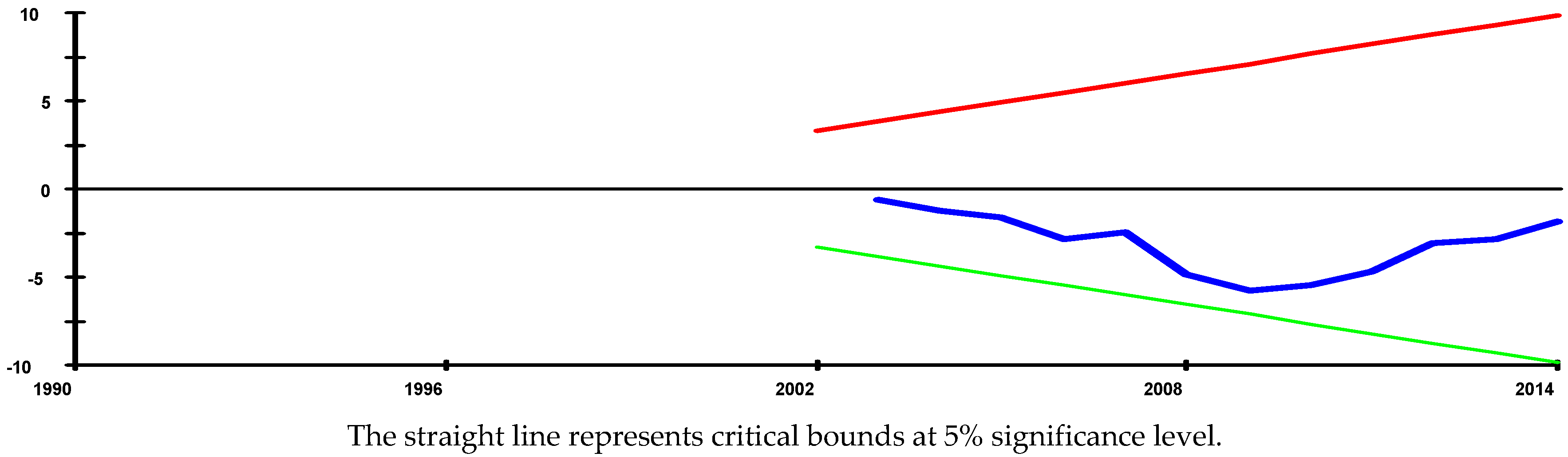
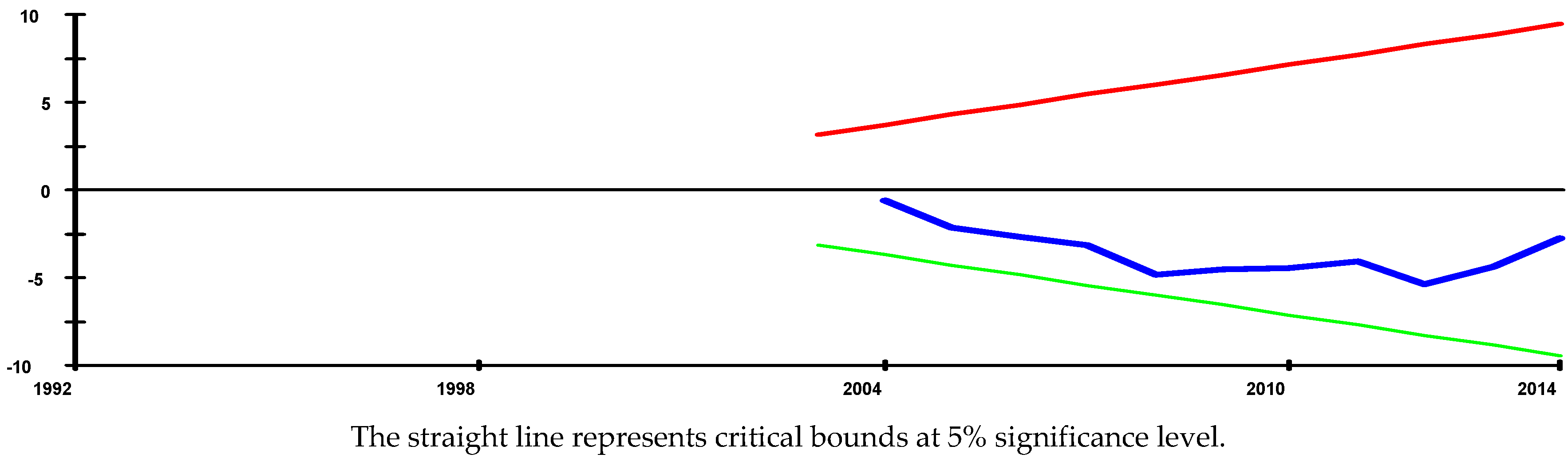
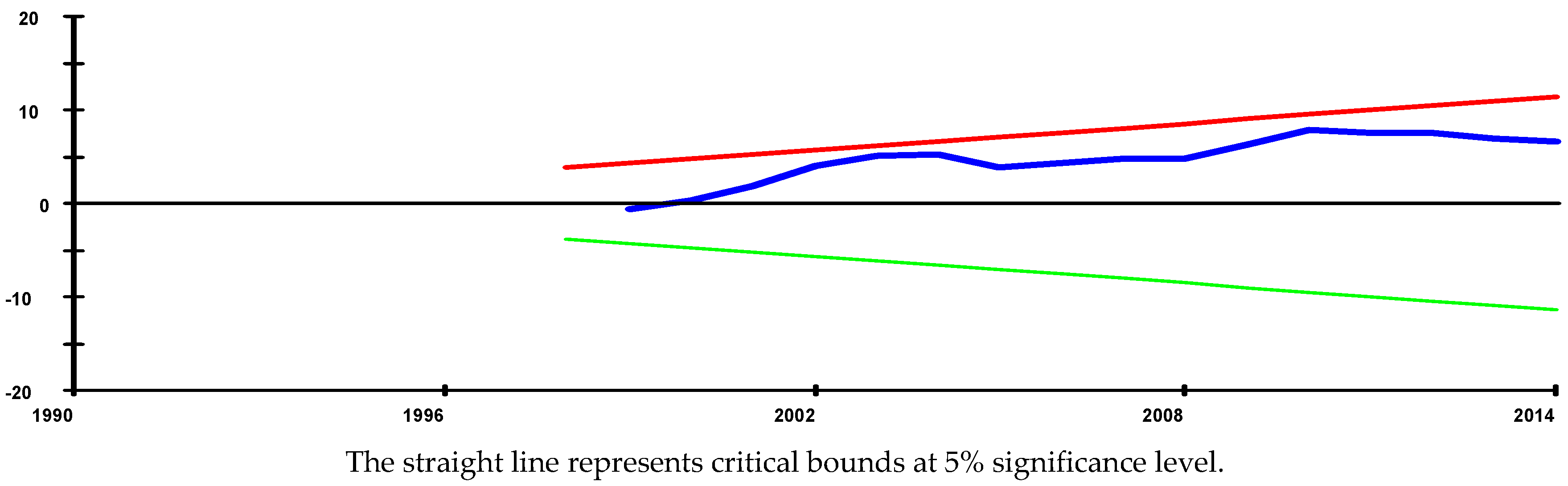
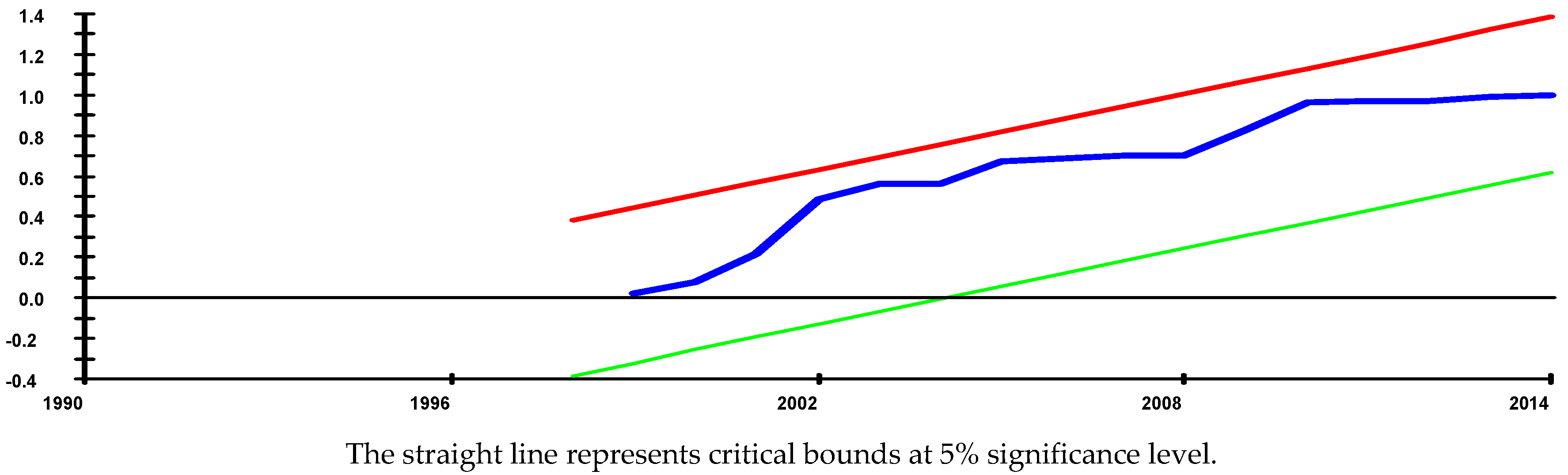
The short-term effects in the above equations are captured by the coefficients of the first differenced variables in the UECM model. According to Bahmani-Oskooee and Brooks (1999 [
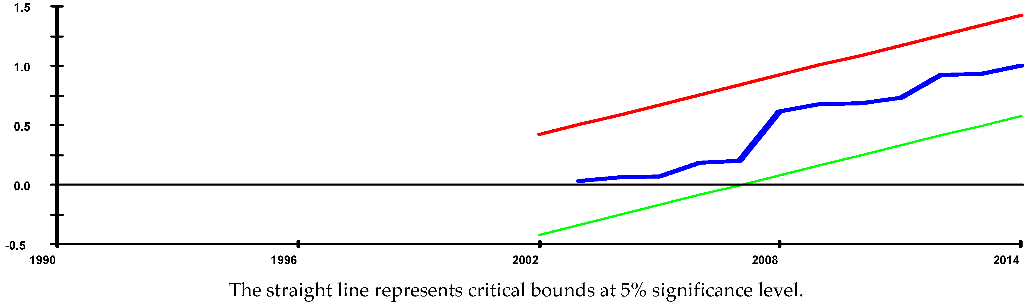
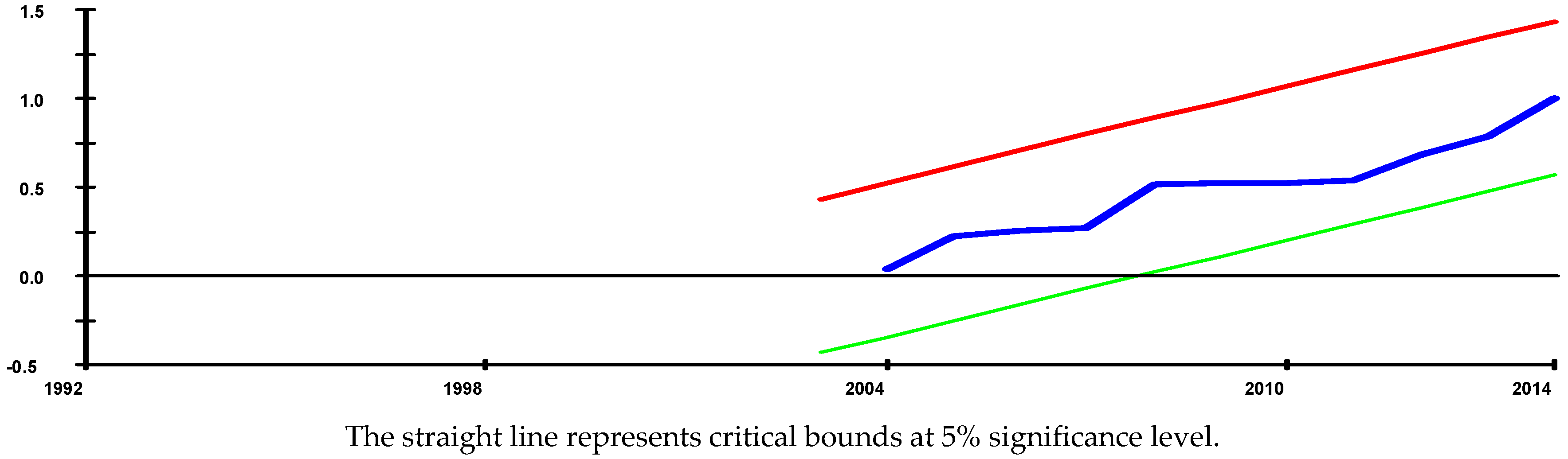
25]), the existence of a long-term relationship does not necessarily imply that the estimated coefficients are stable. This, therefore, implies that there is the need to perform a myriad of tests diagnoses on the selected model. This involves testing of the residuals for homoscedasticity, serial correlation, etc., as well as stability tests to ensure that the estimated model is statistically robust.
The general UECM model is tested downwards sequentially, by dropping the statistically insignificant first differenced variables for each of the equations—to arrive at a “goodness-of-fit” model—using a general-to-specific strategy (Poon, 2010 [
26]; Owusu, 2012 [
20]). Once the co-integration relationships have been established, the long-term elasticities or coefficients can then be generated from UECM (Owusu, 2012 [
20]).


