Abstract
This paper investigates the dynamics of volatility spillovers in the South African foreign exchange market across calm and crisis periods, with particular attention paid to the pre- and post-COVID-19 eras. Employing daily exchange rate returns from 2015 to 2025, we apply a Quantile Vector Autoregression (QVAR) model to uncover asymmetries in spillover transmission across the distribution of returns. We evaluate the implications of these spillovers for portfolio performance under three canonical strategies: risk parity, tangency, and naïve equal-weighting. Our findings indicate that the COVID-19 shock intensified volatility spillovers and exacerbated their asymmetry, especially in the lower tail, while the pre-COVID period portrayed higher volatility compared to the post-COVID period under calm market conditions. While risk-based strategies dominate in tranquil markets, equal-weighted portfolios exhibit superior downside resilience under stress, although they ignore risk exposure. These results underscore the importance of accounting for tail-risk-driven interconnectedness in portfolio construction and risk management. This study contributes to the growing literature on volatility spillovers and offers practical insights for managing currency exposure in emerging markets under nonlinear dependence structures.
1. Introduction
The South African foreign exchange market has been characterized by persistent volatility and prolonged depreciation of the rand for over two decades, a trend that has significantly disrupted key economic fundamentals such as production, trade flows, capital mobility, and investment patterns (Chikwira & Jahed, 2024; Maveé et al., 2016). These exchange rate fluctuations are often amplified during periods of global or regional crises, with heightened volatility impeding diversification opportunities and exacerbating downside risk exposures (Diebold & Yilmaz, 2015). In addition, the dynamics of exchange rate volatility in South Africa have gained renewed importance in the post-COVID-19 era due to intensified disruptions both domestic and international that include load-shedding, global risk aversion, and monetary policy changes (SARB, 2023). According to the International Monetary Fund (IMF, 2020a), these dynamics have also adversely impacted foreign direct investment (FDI) inflows into South Africa, raising concerns about macroeconomic resilience and investor confidence. Against this backdrop of heightened uncertainty and increased integration into global capital markets, the South African Reserve Bank (SARB, 2020) shows that understanding the transmission mechanisms of exchange rate volatility is critical particularly during turbulent periods when policy space narrows and financial contagion risks intensify. Moreover, for an emerging market such as South Africa, whose external sector remains sensitive to exogenous shocks, insights into how foreign exchange volatility spills across currency pairs and over time is essential for investors, policymakers, and international stakeholders.
A growing body of research has attempted to quantify exchange rate volatility and its transmission dynamics using standard models. These include Vector Autoregressive (VAR) models (Boakye et al., 2023), Autoregressive Distributed Lag (ARDL) models (Mpofu, 2021; Ngondo & Khobai, 2018), and the family of Generalized Autoregressive Conditional Heteroskedasticity (GARCH) models (Buthelezi, 2023). While such models have proven useful in capturing linear interdependencies and short-run dynamics, their assumptions of normality and symmetry often fall short during periods of financial stress, where heavy tails, regime shifts, and nonlinear dependencies prevail. As Diebold and Yilmaz (2015) emphasize, accurately identifying volatility spillovers is imperative for informing portfolio allocation and macroprudential risk management strategies. Despite methodological advances, there remains a critical gap in the literature regarding the quantile-specific framework of volatility transmissions, particularly in the South African foreign exchange context. Most existing models implicitly assume homogeneous effects across the distribution of returns, thereby neglecting the asymmetric impact of volatility under extreme conditions1. This limitation is particularly more significant during periods of increased volatility in the global economy, where tail risks have become more pronounced.
The COVID-19 pandemic introduced a distinct set of financial and real economy shocks that differ meaningfully from those experienced in the pre-COVID period. Whereas the pre-COVID era was characterized by moderate disruptions (Goldstein et al., 2021), the post-2020 environment has been shaped by compounded crises, including a global health crisis, escalating geopolitical tensions in Europe, and military conflicts in the Middle East. These developments, especially through their impact on trade and capital flows, have further weakened South Africa’s current account balance and amplified exchange rate instability. Notably, these events have highlighted the limitations of conventional models that do not account for market asymmetries or extreme-state dependencies. Moreover, prior studies often fail to distinguish between different market states. This omission is non-trivial especially in stable and distressed markets. Under bullish conditions, investor optimism tends to suppress perceived risks and dampen exchange rate volatility, thereby reducing the urgency of spillover monitoring for policy or portfolio rebalancing (Škrinjarić et al., 2020). Conversely, under stable and distressed conditions, volatility spillovers become materially significant as they influence import/export pricing, currency mismatch risk, and sovereign debt exposure, particularly in emerging markets (Bernoth & Herwartz, 2021). Thus, this study focuses on the volatility spillover dynamics and portfolio performance under stable and bearish market conditions.
To address these gaps, this paper applies the Quantile Vector Autoregressive (QVAR) model to examine exchange rate return spillovers across different quantiles of the conditional return distribution. The QVAR model is particularly well-suited to capture distributional heterogeneity, non-normality, skewness, and kurtosis, which are often observed in financial return series during stress periods. By contrasting QVAR outcomes with those from traditional VAR models, the study delivers a more nuanced analysis of asymmetric volatility transmission in the South African rand (ZAR) vis-à-vis its major trading partner currencies, including the US dollar (USD), Chinese yuan (CNY), Brazilian real (BRL), Japanese yen (JPY), Botswana pula (BWP), and the euro (EUR). Furthermore, this study distinguishes volatility transmission patterns across pre- and post-COVID periods, shedding light on how crisis heterogeneity affects currency market interdependence. Particular attention is devoted to the dynamics of volatility spillovers under stable and distressed regimes, where the implications for hedging, reserve adequacy, and policy signalling are most pronounced.
The principal objective of this study is to investigate the quantile-dependent volatility spillover dynamics in the South African foreign exchange market using the Quantile Vector Autoregressive (QVAR) framework. By adopting this method, this paper aims to capture the heterogeneity in spillover intensities that manifest under different market conditions, particularly in the lower tails of the return distribution. This objective responds directly to the empirical and policy imperative of identifying non-linear and asymmetric risk transmission channels in times of financial distress. The study also seeks to evaluate the comparative effectiveness of QVAR vis-à-vis traditional VAR models in capturing inter-currency dependencies, thereby offering more robust tools for portfolio diversification, policy calibration, and financial stability assessments in highly volatile emerging markets such as South Africa.
Considering the observed shortcomings in the conventional modelling of exchange rate dynamics, especially under non-normal and asymmetric conditions, this paper seeks to answer several critical research questions. First, how does the transmission of exchange rate volatility in South Africa vary across different segments of the return distribution, particularly in the lower tail where market distress is most severe? Second, do volatility spillovers differ across periods of market calm and stress, and how are these period-specific effects distributed across South Africa’s key bilateral currency pairs? Third, to what extent do quantile-specific measures of connectedness enhance our understanding of cross-currency risk interdependence beyond what is captured by traditional mean-based models such as VAR? Finally, how do these quantile-based spillovers inform the design of portfolio strategies and macroprudential interventions aimed at risk mitigation in emerging markets?
Key findings reveal important quantile-specific differences. While both dynamic VAR and QVAR produce similar connectedness indices under stable market conditions, QVAR uncovers significant asymmetries under extreme conditions. In tranquil and stressed markets, the ZAR.CNY and ZAR.USD pairs emerge as net volatility transmitters during both, pre-COVID and post-COVID periods, and ZAR.BWP and ZAR.BRL as net volatility receivers. However, compared to the pre-COVID period, volatility spillovers are higher during market downturns of the post-COVID period. Among all pairwise interactions, ZAR.CNY consistently exhibited the strongest spillover magnitude. Impulse response functions further confirm that ZAR.CNY shocks are persistent, often extending beyond two trading days. Portfolio optimisation results highlight the superior diversification benefits of risk parity strategies during crisis years such as 2016 and 2022. However, negative Sharpe ratios across both periods underscore the inadequacy of returns in compensating for elevated risk exposure.
2. Literature Review
Exchange rates are pivotal to the macroeconomic performance of emerging economies, particularly through their influence on trade competitiveness, capital flows, and financial stability. In the South African context, Ngondo and Khobai (2018) employed an Autoregressive Distributed Lag (ARDL) model to show that exchange rate fluctuations significantly impacted key macroeconomic variables, including exports, imports, capital flows, and industrial production. The appreciation of the South African rand (ZAR) following increased export demand further illustrates the exchange rate’s sensitivity to trade balances (McCloud et al., 2024). Meanwhile, Yeboah and Takacs (2019), using a random effects model, documented how exchange rate volatility adversely affected firm-level profitability among South Africa’s listed companies. Crucially, the transmission of global shocks to the ZAR has material consequences for South Africa’s economic stability. Boakye et al. (2023), using a Vector Autoregressive (VAR) framework, observed a 20% depreciation in the ZAR during the 2013–2016 global crises, with regional repercussions given South Africa’s role as a leading investor on the continent. This underscores the broader implications of currency shocks beyond national borders.
Volatility in the South African foreign exchange market has been a persistent concern. Mpofu (2021), applying both ARDL and GARCH methodologies, demonstrated how adverse exchange rate shocks perpetuate volatility over multiple periods. Similarly, Buthelezi (2023) used a combination of GARCH and Vector Error Correction (VEC) models to reveal that the South African currency market remains highly susceptible to exogenous shocks. Volatility spillovers between asset classes have also been documented. Rai and Garg (2022), using DCC-GARCH and BEKK-GARCH models, found long-run dynamic correlations between exchange rates and stock markets in several BRICS countries, including South Africa. These correlations are especially relevant during episodes of financial distress when volatility transmission is amplified.
Many recent studies have examined the post-COVID landscape of foreign exchange markets in emerging economies. The African Development Bank (ADB, 2021) reported substantial currency depreciations due to reduced foreign direct investment, remittances, and portfolio flows. South Africa endured the most of the pandemic’s economic fallout, accounting for 38% of Africa’s COVID-19 cases in 2021 (Anyanwu & Salami, 2021). The impact of the COVID-19 pandemic on financial markets is also seen to persist in other emerging economies for example, in Indonesia, an emerging economy like South Africa (Hartono et al., 2024). Structural vulnerabilities, such as persistent current account deficits (Fowkes et al., 2018; SARB, 2024; Bureau for Economic Research, 2025), and post-pandemic trade imbalances further exposed the ZAR to external pressures (Monamodi, 2024). High correlations in FX markets during crisis periods have exacerbated financial policy uncertainty (Aftab et al., 2024) and raised the risk of contagion. This is consistent with findings by Diebold and Yilmaz (2015), who argue that elevated connectedness is associated with systemic fragility. For example, Chang et al. (2024) found that exchange rate volatility Granger-caused equity market fluctuations in Taiwan, while Rakshit and Neog (2022) reported a dampening effect on stock returns in other emerging markets.
While GARCH and ARDL models remain widely used, they are fundamentally mean-based and hence limited in their ability to account for skewness, heavy tails, or asymmetric transmission mechanisms. ARDL models, although effective for long-run co-integration analysis (Begum et al., 2022), are ill-suited to capture extremal co-movements or tail dependencies that typify financial distress periods. GARCH-type models, focused on conditional variance, often rely on strong distributional assumptions and can underperform in the presence of non-Gaussian distribution (Engle, 1982). VAR models, similarly, operate under linearity and symmetry assumptions (Lütkepohl, 2005), and do not accommodate structural changes or distributional shifts that are common during market crises. These limitations motivate the application of more flexible, distribution-sensitive frameworks, particularly for understanding the complex dynamics of exchange rate volatility in crisis-prone economies such as South Africa.
The Quantile Vector Autoregressive (QVAR) model, introduced by White et al. (2015), represents a significant methodological advancement by estimating the conditional quantiles of the joint distribution of macro-financial variables. Unlike mean-based approaches, QVAR models capture the entire conditional distribution, thus enabling the analysis of heterogeneous effects across the distribution especially in the lower and upper tails. This feature makes QVAR particularly effective for analysing downside risks, tail dependence, and asymmetric volatility transmission during periods of market stress (Adrian et al., 2019). Koenker and Xiao (2006) further argue that the related Quantile Autoregressive (QAR) models are robust in the presence of asymmetric returns distributions, a feature common in financial data. Gong et al. (2023) and Huang and Zhang (2024) demonstrate that QVAR models can effectively capture asymmetric shock propagation, especially under crisis conditions. In this regard, QVAR facilitates a more accurate representation of tail risk dynamics and inter-market spillovers compared to traditional methods. A recent similar study that applied the QVAR model on exchange rates of emerging economies involved the utilisation of Latin American currencies against major international currencies. This study revealed that during crises, the direct influence of major international currencies on Latin American exchange rates diminishes, albeit with mixed impact on different economies with the Argentinian and Uruguayan pesos receiving shocks, while the Brazilian real and the Peruvian sol were predominantly transmitters of volatility (Kyriazis & Corbet, 2024).
As shown above, much of the literature on exchange rate dynamics in South Africa has relied on ARDL, VAR, and GARCH models, often with a focus on mean of the distribution or long-run equilibrium conditions. However, this approach fails to capture the asymmetric and non-linear responses observed in high-volatility episodes such as the COVID-19 crisis. Given the increased investor interest in emerging market FX markets (Rehman et al., 2022), a country-specific quantile-based analysis is both warranted and timely. This study contributes by implementing both mean-based VAR and QVAR models to examine volatility spillovers in the ZAR during the pre- and post-COVID periods. This dual modelling strategy allows us to compare volatility dynamics at the mean, median, and lower tail of the distribution, capturing extreme downside risks more effectively. We further extend the analysis through portfolio construction and backtesting of ZAR exchange rates with South Africa’s major trading partners, aligning with Basel III recommendations on capital adequacy and risk evaluation (Taskinsoy, 2022).
Understanding the dynamics of exchange rate volatility is imperative for policymakers and investors. As Özdemir (2024) highlights, spillover analysis reveals the origin of financial risk and provides a basis for targeted policy responses. Our QVAR-based approach enables a more accurate stress-testing framework, allowing regulators to assess how exchange rate shocks propagate under adverse conditions. For portfolio managers, this provides actionable insight into downside risk and informs asset allocation strategies under crisis scenarios.
3. Methodology
We employ the Dynamic Time Warping (DTW) distance metric to reduce the dimensionality of the dataset by identifying exchange rates that are dissimilar in their temporal dynamics. Exchange rates with lower similarity, interpreted as being less correlated, are retained for further analysis, in line with portfolio diversification theory, which favours low-correlation assets to mitigate overall portfolio volatility without sacrificing expected returns (Reinholtz et al., 2021). For the empirical investigation of volatility spillovers and portfolio dynamics, we estimate both the Vector Autoregressive (VAR) and Quantile Vector Autoregressive (QVAR) models. The QVAR framework, which models the conditional quantiles of the return distribution, is particularly advantageous in the presence of non-Gaussian features such as skewness and fat tails. Unlike the VAR model, which relies on the conditional mean and is thus more sensitive to outliers and distributional asymmetries, the QVAR provides a robust characterization of dependent structures by focusing on the median, thereby offering a more representative central tendency under such conditions (Prasad, 2023).
3.1. Dynamic Time Warping Distance
Dynamic Time Warping (DTW) is widely employed as a distance-based algorithm to quantify the similarity between time series by aligning their shapes and measuring the optimal warping path between them (Liu et al., 2024; Suris et al., 2022). In the context of portfolio selection, investors often seek assets with lower co-movement to enhance diversification benefits, particularly during periods of market stress when asset correlations increase significantly and prices fall simultaneously, phenomena prominently observed in the aftermath of the COVID-19 crisis (Li et al., 2022). Such episodes of heightened synchronicity have also characterized exchange rate markets, primarily due to elevated economic and policy uncertainty (Aftab et al., 2024). Moreover, elevated cross-asset correlation is frequently associated with spikes in volatility (Diebold & Yilmaz, 2015), and in the case of exchange rates, such volatility has been shown to exert a dampening effect on other aspects of the emerging market economies such as the equity market (Rakshit & Neog, 2022). Against this backdrop, DTW provides a robust methodological framework to identify exchange rate pairs with dissimilar dynamics, facilitating the selection of less-correlated currencies and thereby improving portfolio resilience during turbulent periods. DTW method is given in Suris et al. (2022) as follows:
Given any two time series, and with lengths and in (1) and (2), respectively,
an distance matrix can be obtained where the elements comprise of as the distance between two points. Dynamic programming is then is used to compute the cumulative distance matrix by applying the reiteration in (3).
where is cumulative distance, is the distance of the current cell and the rest of the formula is the minimum value of the adjacent elements of the respective cumulative distance. For a path that minimises the total cumulative distance between the two sequences and that results into the best alignment, to be achieved, three conditions of boundary, continuity, and monotonicity shown below must be satisfied to obtain the warping path.
- (i)
- and ;
- (ii)
- and and ;
- (iii)
- and .
Hence, the DTW distance in (4) is the path that minimizes the warping cost:
In this paper, we applied the DTW distance and hierarchical clustering type for asset similarity analysis. Clustering has often been used to find patterns in datasets consisting of many time series and simplifying them (Aghabozorgi et al., 2015; Guijo-Rubio et al., 2018).
3.2. Generalized Spillover and Measurement in a VAR Model
Diebold and Yilmaz (2012) extend their 2009 spillover index, derived from the variance decomposition associated with an -variable vector autoregression and whose focus was on total spillovers in a simple Vector Autoregressive (VAR) framework to the one which measures the directional spillovers in a generalized VAR framework that eliminates the possible dependence of the results on ordering. This model, whose detailed discussion is given in Diebold and Yilmaz (2012), is as follows:
Based on the famous work of Sims (1980), the covariance stationary -variable in Diebold and Yilmaz (2012) is given in (5) as:
where are independently and identically distributed (iid) innovations, the moving average representation is , where the coefficient matrices obey the recursion , with being an identity matrix and with for . The moving average coefficients (or transformations such as impulse response functions or variance decompositions) are used to dissolve the forecast error variances of each variable into parts responsible for various system shocks through the assessment of the fraction of the H -step-ahead error variance in forecasting that is due to shocks to , for each .
Computing variance decompositions requires orthogonal innovations which are achieved by employing the generalized VAR framework of Koop et al. (1996) and Pesaran and Shin (1998), hereafter KPPS, which produces order-invariant variance decompositions. Instead of orthogonalizing shocks, this approach allows correlated shocks but accounts for them using the historically observed error distributions. As the shocks to each variable are not orthogonalized, the sum of the contributions to the variance of the forecast error may not be equal to one.
3.2.1. Variance Shares
Diebold and Yilmaz (2012) define variance shares as the fractions of the -step-ahead error variances in forecasting attributed to shocks to , for , and cross variance (spillovers) as the fractions of the -step-ahead error variances in forecasting that are due to shocks to , for , .
Denoting the KPPS -step-ahead forecast error variance decompositions by in (6) for ,
where is the variance matrix for the error vector , is the standard deviation of the error term for the th equation, and is the selection vector with th element 1 and zeros otherwise. Because the sum of the elements in each row of the variance decomposition table, , to use the information available in the variance decomposition matrix in the calculation of the spillover index, each entry of the variance decomposition matrix is normalized by the row sum as:
By construction, and .
3.2.2. Total Spillovers
Using the volatility contributions from the KPPS variance decomposition of the Cholesky factor-based measure, total volatility spillover index is calculated in (8) as:
The total spillover index measures the contribution of spillovers of volatility shocks across all assets to the total forecast error variance.
3.2.3. Directional Spillovers
Whereas the total volatility spillover index shows the number of shocks to the volatility spillover across all assets, the generalized VAR approach facilitates the understanding of the direction of volatility spillovers across all assets. As the generalized impulse responses and variance decompositions are order-invariant, directional spillovers received by asset from all other assets , are calculated using the normalized elements of the generalized variance decomposition matrix, as shown in (9).
Similarly, the directional volatility spillovers transmitted by asset to all other assets are calculated as:
3.2.4. Net Spillovers
Net volatility spillover from asset to all other assets , measured by the difference between the gross volatility shocks transmitted to and those received from all other assets, is calculated in (11) as:
3.2.5. Net Pairwise Spillovers
Unlike the net volatility spillover in (11), which provides information about how much each asset contributes to the volatility in other assets in net terms, the net pairwise volatility spillovers in (12) provide the difference between the gross volatility shocks transmitted from asset to asset and those transmitted from to .
3.3. Quantile Vector Autoregressive Model and Spillovers
Quantile vector Autoregressive (QVAR) model and spillover model, whose detailed discussion is provided in Khalfaoui et al. (2023) and Ando et al. (2022), are used to measure the spillover connectedness of variable ) on variable (independent) at the th quantile, where of the conditional distribution . The QVAR model of order and dimension can be written as follows:
where is vector of dependent variables, denotes the lag length, is the mean vector of order at the quantile is the matrix of quantile VAR coefficients of order , and are the residual terms at quantile . Based on Wold theorem, the quantile moving average in (13) can be expressed as:
Ando et al. (2022) extend the mean-based quantities of Diebold and Yilmaz (2012) to more flexible estimates of return connections among quantiles, . This connectedness is further extended by Jena et al. (2022) to incorporate an infinite order vector-moving average shown in (15).
where
and
In (15), variable can be expressed as the sum of the error terms . Then, to determine the impact of spread in asset on asset , the H-variates ahead Generalized Forecast Error-Variance Decomposition (GFEVD) are calculated in (18) by Chatziantoniou et al. (2021) as:
where refers to the th asset’s contribution to the variance of the forecasting error of the th asset at horizon , matrix, denotes the variance matrix for the residual vector and is the th diagonal component of the matrix, . Vector assigns a vector with value 1 at the th component and 0 otherwise.
The normalized variance decomposition matrix is calculated in (19) as:
GFEVD is then used to quantify the degree of connectedness at each quantile. In Diebold and Yilmaz (2012), to assess the overall spillover impact in the entire system, the total spillover connectedness index (TCI) at quantile is calculated in (20) as:
To measure the spillover effect of asset from all other assets at each quantile , the “FROM” and “TO” measures are used, with the th directional spillover index “FROM” given in (21) as:
And the th directional spillover index “TO” is expressed in (22) as:
From the directional spillover index measures “FROM” and “TO”, the th net spillover index (NET) is calculated in (23) as the difference between “TO” and “FROM” measures.
Lastly, the th net pairwise directional connectedness (NPDC) spillover index in (24) is defined as:
3.4. Model Stability Test
According to (Pfaff & Stigler, 2024), a VAR(p)-process in its companion form is stable if its reverse characteristic polynomial in (25),
has no roots in or on the complex circle. This satisfies the condition that all eigenvalues of the companion matrix have modulus less than 1. The function roots in the vars package is used to compute the eigenvalues of the companion matrix A and return their moduli.
3.5. Portfolio Optimization
In this study, we conduct portfolio optimization following the estimation of both the VAR and QVAR models across the pre- and post-COVID-19 periods. To ensure robustness, we implement three well-established portfolio allocation strategies: the risk parity portfolio, the tangency portfolio, and the naïve equally weighted portfolio (EWP). The risk parity approach, while analytically intricate due to its non-linear structure, offers a theoretically sound framework for risk-based asset allocation (Roncalli, 2013). Recent advances in computational methods have significantly reduced the practical barriers to implementing this technique. The tangency portfolio, grounded in mean-variance optimization and maximizing the Sharpe ratio, remains a benchmark model widely adopted in the investment community for its theoretical elegance and empirical performance (Surtee & Alagidede, 2023). Meanwhile, the equally weighted portfolio, despite its simplicity, continues to garner empirical support for its out-of-sample performance and diversification benefits, particularly in the face of model estimation risk (Shabani et al., 2024). Leveraging these methodologies, we evaluate and compare the performance of each portfolio strategy through the analysis of Sharpe ratios and portfolio backtesting.
3.5.1. Risk Parity Portfolio Optimization
Risk parity portfolios (RPP) are equally weighted risk contribution (ERC) portfolios that imitate the diversification contributions of equally weighted portfolios while considering single and joint risk contributions of the assets (Maillard et al., 2010). Maillard et al. (2010) define risk parity portfolios in assets, as follows:
Let be the variance of asset be the covariance between assets and and be the covariance matrix. Let be the risk of the portfolio. Thus, marginal risk contributions, , are defined as follows:
where marginal are the quantities that give the change in volatility of the portfolio caused by a small increase in the weight of one component. If total risk contribution of the asset is given as , then we obtain the following decomposition:
Thus, the risk of the portfolio is deducted as the sum of the total risk contributions. A RPP portfolio is optimal if we assume a constant correlation matrix and all assets have the same Sharpe ratio. If the constant correlation coefficient assumption holds, the total risk contribution of asset is equal to and it will be the same for all assets. It is further required that each asset has the same individual Sharpe ratio given as, . However, when the correlations or Sharpe ratios differ, the RPP portfolio will differ from the maximum Sharpe ratio (MSR) portfolio.
3.5.2. Tangency Portfolio Optimization
Tangency portfolio or maximum Sharpe ratio (MSR) portfolio is defined in Maillard et al. (2010) as the portfolio where the ratio of the marginal excess return to the marginal risk is equal for all assets in the portfolio and is the same as the Sharpe ratio of the portfolio as shown in (28):
Therefore, portfolio is MSR if it satisfies the following relationship:
Practically, the tangency portfolio lies on the efficient frontier and with the maximum Sharpe ratio (see Bechis et al., 2020).
3.5.3. Equally Weighted Portfolio
The equally weighted portfolio (EWP) is defined as the portfolio of assets where each asset has the same weight so that all assets in the portfolio have weight given as:
Consequently, from the definition of EWP, each asset has the same weight as other assets in the portfolio. This is a naïve portfolio construction method that does not require any optimization.
3.6. Portfolio Performance Measurement
After constructing portfolios, the Sharpe ratio () is used to measure portfolio performance, where the optimal diversified portfolio is the one that maximizes the Sharpe ratio (Pav, 2021) and the annualized Sharpe ratio is given in Equation (31) as:
where is the mean of portfolio returns, is the risk-free rate of return and is the standard deviation of and a measure of portfolio risk. Thus, the Sharpe ratio captures a tradeoff between objectives of maximizing expected returns and minimizing risk and asset weights () are selected by the optimizer to achieve these objectives.
3.7. Portfolio Backtest
According to the Basel III framework of the Basel Committee on Banking Supervision (BCBS), portfolios should be backtested to assess the accuracy of risk models and ensure capital adequacy (Taskinsoy, 2022). Backtesting can be analysed using portfolioBacktest package (version 0.4.1) where statistical results of the executed backtest that include the cumulative return and the maximum drawdowns, are provided (Sarasa-Cabezuelo, 2023).
4. Empirical Findings
This study employs both standard Vector Autoregressive (VAR) and Quantile Vector Autoregressive (QVAR) frameworks to investigate the dynamic relationships among selected exchange rates under stable and bear market conditions. Preliminary analyses are presented prior to the main empirical results, which encompass volatility spillover dynamics, asset-specific and portfolio-level performance assessments, and portfolio backtesting. The analysis compares the pre-COVID and post-COVID periods using log-returns data from eight bilateral exchange rates, each expressed as the South African Rand (ZAR) vis-à-vis the currencies of key trading partners and some BRICS counterparts. Specifically, the currency pairs include ZAR/BRL2, ZAR/RUB, ZAR/INR, ZAR/CNY, ZAR/EUR, ZAR/JPY, ZAR/USD, and ZAR/BWP, wherein the foreign currency serves as the base and ZAR as the quote currency. This construction facilitates an assessment of asymmetric spillover transmission and performance heterogeneity across different economic regimes and market conditions. To achieve more diversified portfolios, the similarity of exchange rates is analysed, and less similar exchange rates are retained.
Exchange rate data was obtained from the investing.com website and consists of daily closing prices of exchange rates from 5 January 2015 to 5 March 2025 with 1302 and 1351 observations for the pre- and post-COVID periods, respectively. We calculate the log-returns of daily closing prices using where is the price of the financial asset, i at time, .
Exchange rate prices in Figure 1 show trends in the data, an indication of non-stationary series and therefore we extract the non-trending asset returns data for the analysis. Line plots of exchange rate prices and returns show co-movement in both pre- and post-COVID periods, and except for 2016, are characterized by higher volatility in the post-COVID period. The highest volatility in the post-COVID period is recorded during the first six months of 2020 when the COVID-19 crisis was at its peak.
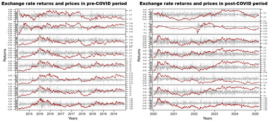
Figure 1.
Exchange rate prices (red) and returns (gray) for the pre- and post-COVID periods where the left y-axis represents exchange rate returns and the right y-axis represents exchange rate prices.
Preliminary descriptive statistics of the daily log-returns of exchange rates, as reported in Table 1, reveal significant departures from normality, specifically, pronounced skewness and excess kurtosis, highlighting the presence of heavy tails and asymmetries in the distribution of returns. Considering these distributional features, we employ the Quantile Vector Autoregression (QVAR) model, which is robust to deviations from normality and less sensitive to skewness and kurtosis in the data-generating process. The results derived from the QVAR specification are juxtaposed with those from the conventional Vector Autoregression (VAR) framework, which is more susceptible to such statistical irregularities. Furthermore, the standard deviation statistics indicate that exchange rate volatility was higher during the pre-COVID period relative to the post-COVID period. However, it is important to note that the summary statistics in Table 1 reflect average volatility over the sample windows and may obscure episodic surges in volatility that occurred in sub-periods of the post-COVID era, which at times surpassed those observed in the pre-COVID phase.

Table 1.
Summary statistics.
In Table 1, all Jarque–Bera statistics in both periods have p-values < 0.001 and thus, at degree of freedom (df = 2), the null hypothesis of normally distributed residuals is rejected. For estimation purposes, the least squares estimators of the coefficients in a VAR model will be consistent and asymptotically normal under very general conditions and thus not requiring normality of the residuals (Lütkepohl, 2013). The augmented Dickey–Fuller (ADF) statistics for all exchange rate returns in both periods have p-values < 0.01 and with a lag order of 10 and 11 for the pre- and post-COVID periods. Thus, the null hypothesis of non-stationary returns for the ADF test is rejected. Modelling asset returns requires stationarity to ensure valid statistical inference and risk measurement (Tsay, 2010). Ljung–Box autocorrelation test results show that with a 5% confidence level and p < 0.05, the null hypothesis of no autocorrelation is not rejected for most of the exchange rate returns, especially in the pre-COVID period. Lütkepohl (2005) ascertains that in the presence of autocorrelation or dynamic interdependence among the variables, VAR models are suitable for analysing multivariate time series.
Given the non-normality of the exchange rate return distributions, Spearman’s rank correlation coefficient is employed as a more robust measure of dependence than Pearson’s correlation, which assumes linearity and normality in the underlying data (Bishara & Hittner, 2017). As depicted in Figure 2, all correlation coefficients are statistically significant at the 5% level. Notably, while the ZAR/BRL and ZAR/RUB exchange rate pairs exhibit persistently low correlations across both the pre- and post-COVID periods, the remaining bilateral exchange rates involving South Africa’s primary trading partners, namely the USD, EUR, CNY, INR, JPY, and BWP demonstrate relatively high degrees of co-movement. This pattern of cross-market co-movements suggests a potential concentration risk for investors. Therefore, portfolio diversification strategies aiming to mitigate downside exchange rate risk may benefit from incorporating lower-correlated currency pairs such as ZAR/BRL or ZAR/RUB alongside more volatile or highly correlated currencies (such as ZAR/USD or ZAR/EUR). The rationale is that the low pairwise correlations reduce the likelihood of concurrent adverse currency movements, thereby improving hedging effectiveness and enhancing the diversification benefits within multi-currency portfolios (Zaimovic et al., 2021).
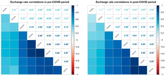
Figure 2.
Correlations ordered based on hierarchical clustering and using Spearman’s rho (ρ) correlation measure. (*) corresponds to p ≤ 0.05, where p are the p-values. The lower triangle shows correlations as represented by the intensity of the colours where higher intensity signifies higher correlation and the upper triangle shows Spearman’s rank correlation values.
In constructing diversified and cost-efficient portfolios, investors often face the challenge of selecting a parsimonious subset of assets from a broader set, that has low transaction costs and achieves diversified and optimal portfolios (Gunjan & Bhattacharyya, 2023). To address this, we employ the Dynamic Time Warping (DTW) distance metric to evaluate the temporal similarity of exchange rate return series, under the rationale that including less synchronized exchange rates mitigates the risk of excessive co-movement within the portfolio. As shown in Table 2, the DTW analysis reveals strong alignment between the exchange rate pairs of ZAR/RUB and ZAR/INR, ZAR/JPY and ZAR/INR, as well as ZAR/JPY and ZAR/RUB. To reduce dimensionality and enhance portfolio diversification, we exclude ZAR/RUB and ZAR/INR from the spillover and portfolio analyses and retain ZAR/JPY. This choice is further justified on the grounds that, relative to India and Russia, Japan constitutes a more significant trading partner for South Africa (SARB, 2024).
Table 2.
Similarities of exchange rates.
Extending the study of Iyke and Ho (2021), we analyse the relationships between exchange rates in pre- and post-COVID periods. First, we carry out the Granger causality test after fitting the VAR model. Although this test does not imply true causality, it shows that past values of one time series contain information that helps predict the other time series (Granger, 1969). Granger causality test results in Appendix A Table A1 and at 5% significance levels show that in the pre-COVID period, only in 10 out of 30 exchange rate pairs the null hypothesis of non-causality is rejected. Therefore, in these 10 pairs, where we denote with → the direction of causality, we find that ZAR.BWP→ZAR.BRL, ZAR.CNY→ZAR.BWP, ZAR.EUR→ZAR.BWP, ZAR.JPY→ZAR.BWP, ZAR.USD→ZAR.BWP, ZAR.BRL→ZAR.EUR, ZAR.BRL→ZAR.JPY, ZAR.USD→ZAR.BRL, ZAR.EUR→ZAR.JPY, ZAR.USD→ZAR.JPY. Thus, in the pre-COVID period, other exchange rates can be used to predict the ZAR.BWP exchange rate, but the ZAR.BWP exchange rate cannot be used to predict other exchange rates. ZAR.USD and ZAR.BRL are good predictors for most exchange rates with three apiece, ZAR.EUR with two and ZAR.JPY and ZAR.CNY with one each in this period. In the post-COVID period, out of 30 exchange rate pairs, only in 6 pairs the null hypothesis is rejected. In this period, there is reversal causality of ZAR.BRL→ZAR.BWP and ZAR.BWP→ZAR.EUR, a new causality of ZAR.CNY→ZAR.JPY, and unchanged causalities of ZAR.BWP→ZAR.EUR, ZAR.BWP→ZAR.JPY, ZAR.BWP→ZAR.USD. In both periods, ZAR.BWP can be used to predict other exchange rates but other exchange rates cannot be used to predict the ZAR.BWP exchange rate. ZAR.JPY, and ZAR.BRL are good predictors for other exchange rates with three apiece. The bellwether impact of the ZAR.BWP exchange rate may emanate from pegging the Pula to the Rand (Badimo & Yuhuan, 2025), and the prominent role of South Africa and Botswana as top-tier producers of precious metals and diamonds (Pinto, 2020), for which larger emerging and developed economies are the major consumers (Merem et al., 2021), and thus are subjected to currency exposure due to changes in prices of these commodities.
We proceed the analysis with exchange rate volatility spillover effect where the results of model are compared to those of and at 50% and 5% quantile levels where the former represents the median and the later represents the lower tail of the exchange rate return distribution. Whereas in the presence of a normal distribution of returns, VAR and may produce similar spillover results (Zhang & Wei, 2024), the results may differ when the data is not normally distributed. Figure 3 plots of network spillover show that exchange rates of much bigger economies (ZAR.CNY and ZAR.USD) are transmitters of volatility to ZAR.BWP, ZAR.BRL and ZAR.EUR for the VAR model in both periods but amongst themselves, the roles reverse with ZAR.USD being a net receiver in the post-COVID period. The results of and are similar, indicating our exchange rates returns data do not deviate from a normal distribution and thus the results of the mean (VAR) and median models are similar. However, under stressed market conditions , the two periods differ substantially, with higher volatility spillovers during the pre-COVID period and with reversed roles for ZAR.JPY and ZAR.EUR, ZAR.CNY and ZAR.USD. According to the IMF report (IMF, 2023), South Africa is exposed to external shocks and capital flow volatility because of its high integration in global financial markets, making the country highly susceptible to global disruptions such as monetary policy tightening by the US that according to Gudmundsson et al. (2022) triggered capital outflows from emerging economies as investors sought higher interest rates. Also, the IMF report (IMF, 2023) shows that domestically, South Africa experienced severe power outages in the years leading up to 2020. This led to lower production, lower exports and lower domestic demand in the pre-COVID era. However, the IMF report adds that the improvement in the country’s power supply in the post-COVID era for example in 2023 led to increased production, exports, and stabilization of the rand.
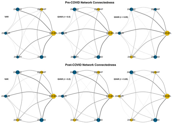
Figure 3.
Network connectedness spillovers where thicker lines indicate higher spillover effects and arrows indicate the direction of the spillover. The analysis of connectedness in this study is carried out using the ConnectednessApproach package of Gabauer and Gabauer (2022).
In addition, because all eigenvalues were less than 1, we confirm that the fitted VAR models are stable.
In contrast to the pre-COVID period, which experienced unrelenting connectedness, the dynamic total connectedness index (TCI) plots in Figure 4 show a decrease in overall foreign exchange market connectedness. This happened between 2022 and 2023 and the last half of 2024 in the post-COVID period under stable market states represented by VAR and models. However, during this period, total connectedness increased between 2023 and 2024, and in the first quarter of 2025, there was an indication of increased volatility risk. Compared to the stable market conditions, under bear market states captured by the model, the overall market experienced the highest connectedness during the pre- and post-COVID periods. Additionally, average TCI values in Table A2 are over 70%, showing high interdependence among all exchange rates for all periods which signals greater downside risk and high transmission of volatility shocks. This, however, has remained at below 74% for all periods except during the post-COVID period under turbulent market conditions. VAR and models show that under stable market conditions, the exchange rate volatility impact from one exchange rate to another for most exchange rates is indistinguishable. Furthermore, we see that the volatility spillover in the pre-COVID period remained higher and more consistent compared to the post-COVID period under stable market conditions. This shows higher integration and higher possibility of risk in the South African foreign exchange market in the pre-COVID period. On the other hand, during bearish market states (), TCI is high and consistently above 80% during both pre- and post-COVID periods. This indicates higher volatility spillovers or higher systemic integration within the South African foreign exchange market under distressed market conditions. Thus, during market downturns, the South African foreign exchange market is riskier compared to a stable market state. As a result, the tendency for the different exchange rates to co-move increases significantly under the distressed foreign exchange market.
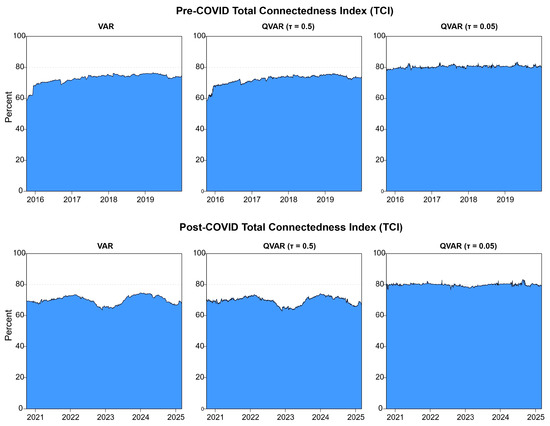
Figure 4.
Dynamic total connectedness plots from the standard VAR (mean), quantile VAR (QVAR) results at 50% quantile (median) and 5% quantile (stressed markets). TCI values range between 0% (no connectedness and thus each exchange rate is self-driven) and 100% (maximum connectedness and thus all exchange rates are entirely driven by others).
The pairwise connectedness index (PCI) plots in Figure 5 show significantly higher varying levels of volatility spillovers compared to total connectedness between the pre- and post-COVID periods for all models with volatility spillovers between ZAR.CNY and ZAR.USD being much higher compared to other exchange rates. PCI index helps determine the direct connectedness between two exchange rates in a system, isolating pairwise relationships rather than aggregate system-wide connections of TCI. Thus, exchange rate pairs are more connected during the pre-COVID period under stable market conditions. However, under bearish market states, although the pre-COVID period is more volatile, the post-COVID period shows higher interconnectedness among exchange rate pairs, especially from larger emerging and developed economies. Thus, the post-COVID period poses a higher risk to investors during market downturns than the pre-COVID period. Thus, the risk of simultaneous losses emanating from exchange rate co-movement is higher when investors are holding currencies of larger emerging and developed economies of China, US, Japan, the Euro zone. But risk is reduced when investors hold a mixture of developing countries’ currencies of Botswana and Brazil and those of larger emerging and developed economies.
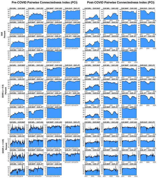
Figure 5.
Dynamic pairwise connectedness plots for standard VAR (mean) plots and quantile VAR (QVAR) results at 50% (median) and 5% (stressed markets).
Table A2 results provide an insight into average individual exchange volatility and PCI spillovers. The diagonal elements indicate own influence of volatility, with BRL having the highest for all models and in all periods. Thus, BRL is the currency that explains the highest of its own variance of 45.49% and 53.26% in the pre- and post-COVID periods, respectively. The results are identical under the stable market state for the VAR and models. For the model, the results remain unchanged in the pre-COVID period with 45.49% for BRL. However, there is a drastic decline for the in the post-COVID period, and BRL only accounts for 22.45% of its own volatility. Off-diagonal elements (spillovers) indicate that except for BRL, movements in the CNY and USD contribute the highest fluctuations of between 15% and 17% to other currencies. In order of magnitude, USD fluctuations are mainly attributed to fluctuations in CNY, JPY, EUR, BWP and BRL. For the EUR, under both periods and with all models, the biggest spillovers emanate from JPN, CNY, USD, BWP and BRL, and remain largely unchanged at between 15% and 18%. Lastly, among the developed economies, fluctuations in the JPY during both pre-and post-COVID periods, and for all models, the biggest fluctuations affecting JPY come from EUR, USD, CNY, BWP and BRL. Among the emerging economies, fluctuations in CNY can be attributed to fluctuations in USD, JPY, EUR, BWP and BRL. For BWP, pre-COVID fluctuations from other currencies are higher than in the post-COVID period, whereas for BRL, post-COVID fluctuations from other currencies are higher than those in the post-COVID period. Hence, spillover results show that the level of integration among the emerging economies of the global south is still low whereas a strong linkage exists among the developed economies. Furthermore, the ‘FROM’ column or ‘from-others’ in Table A2 shows that under turbulent and stable market conditions, as captured by the VAR and and models, BRL and BWP are the biggest receivers of volatility from other currencies of CNY, USD, EUR and JPY. Whereas under stable market conditions BRL and BWP receive comparable volatility with both VAR and QVAR models and both periods, under stressed market conditions, BRL and BWP receive more volatility from larger economies in the post-COVID period. The ‘TO’ column or ‘to-others’ on the other hand shows that, in order of magnitude, the highest transmitters of volatility spillovers are CNY, USD, EUR, JPY, BRZ and BWP for all models and all periods. However, the post-COVID period volatility spillovers to others under the stressed market state has increased substantially compared to that of the pre-COVID period.
Impulse response functions in Figure A1, based on the ZAR.CNY exchange rate as the transmitter, since all impulse for ZAR.USD were statistically insignificant, show that a shock emanating from ZAR.CNY affects all exchange rates except ZAR.BRL where the shocks are not statistically significant. These shocks have an asymmetric impact, with the impact towards ZAR.BWP lasting for about three days compared to two days on ZAR.CNY, ZAR.EUR, ZAR.JPY and ZAR.USD exchange rates.
A more robust analysis is captured by the FEVD plots in Figure 6. In both periods, the origin of the shock to the ZAR.BRL exchange rate is mainly attributed to the ZAR.BRL itself for the entire 10-day horizon period. For the rest of the exchange rates, they are impacted by other exchange rates, with the impact having a lingering effect on that exchange rate.
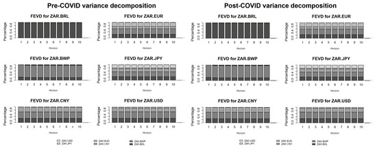
Figure 6.
Variance decomposition plots showing where the shock came from in percentage. FEVD plots are based on the model.
The dynamic net connectedness plots in Figure 7 show that during stable market states as depicted by the and models in both periods, the highest net transmitters of volatility are ZAR.CNY and ZAR.USD, and the highest net receivers of volatility are ZAR.BWP and ZAR.BRL, with mixed results for ZAR.EUR and ZAR.JPY. Under bear market conditions however, ZAR.BRL remains the highest receiver of volatility and ZAR.CNY and ZAR.USD as the biggest transmitters during both pre- and post-COVID periods. The results from the dynamic analysis are corroborated by those of the average net spillovers in Table A2, which show similar net transmitters and receivers of shocks.
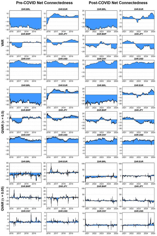
Figure 7.
Dynamic net connectedness plots for standard VAR (mean) model compared to quantile VAR (QVAR) results at 50% and 5%.
In addition to volatility spillover analysis, where we have utilized VAR and QVAR models, we further analyse portfolio performance where we apply risk parity portfolio, tangency portfolio and equally weighted portfolio. The results for individual exchange rate allocations in Figure 8 show that the risk parity portfolio is a better diversified portfolio with most weight being allocated to ZAR.BWP exchange rate and like the equally weighted portfolio, asset weight and risk allocations have not changed much but the allocations in the tangency portfolio have significantly changed with more allocations towards the ZAR.JPY and ZAR.USD during the pre- and post-COVID periods, respectively.
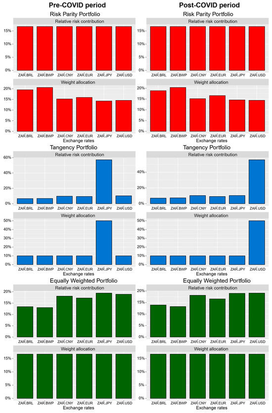
Figure 8.
In the tangency portfolio analysis, constraints of , long_only portfolio and box constraint of min = 0.1 and max = 0.9 are used and objectives of maximizing return and minimizing risk are used.
Cumulative returns in Figure 9 show that 2016 was the most turbulent pre-COVID period with both risk parity and tangency portfolios performing worse than the naïve equally weighted portfolio. The post-COVID period, on the other hand, shows that the worst tumultuous period was the first half of 2022 which corresponds to the beginning of the European political crisis. However, the compounding impact of both the COVID-19 health crisis and the Russian/Ukrainian war has resulted into portfolio underperformance in the post-COVID period compared to the pre-COVID period. This aspect is better captured by the risk parity and tangency portfolios. During both periods, on average the EWP and risk parity portfolio have better diversified portfolios than the tangency portfolio. Maximum drawdowns show that the losses attributed to the EWP portfolio in the post-COVID period are higher than those of risk parity and tangency portfolios. Monthly returns plots show that all portfolios have mainly registered negative returns in the post-COVID period.
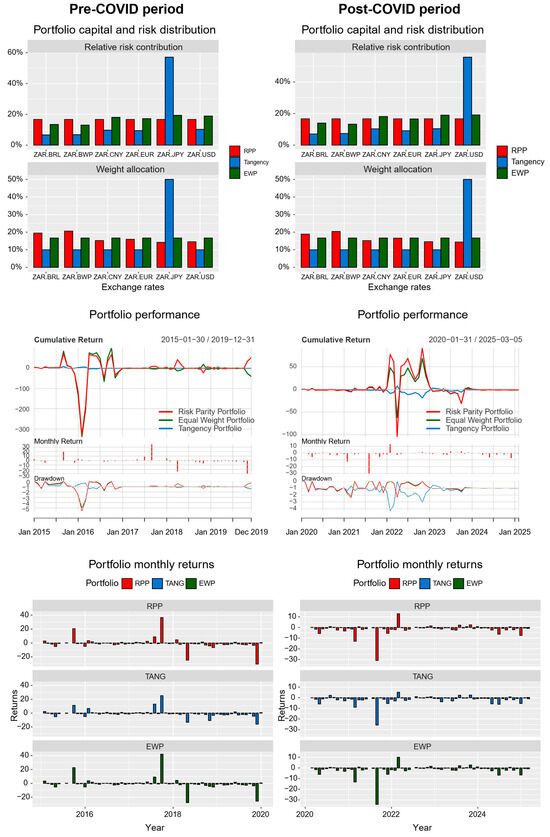
Figure 9.
PortfolioAnalytics, PerformanceAnalytics, xts and portfolioBacktest packages have been used to analyse portfolio performance and backtesting of portfolios.
The performance of all portfolios for each year is shown in Figure 10, where 2017 and 2021 are recorded as riskiest years for each portfolio but during those years, EWP portfolio had underestimated portfolio risk. From 2018 till early 2025, the Sharpe ratio shows that except in 2022 where the performance was marginally positive, other years have recorded negative Sharpe ratios, indicating that investments in the foreign exchange market have not yielded sufficient returns to compensate for the risk taken (see Irfani & Sudrajad, 2023).
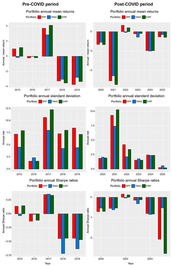
Figure 10.
In the computation of the Sharpe ratio, a zero risk-free rate is used.
5. Discussion
The empirical analysis of exchange rate volatility and portfolio performance across pre- and post-COVID-19 periods reveals marked structural changes in the dynamics of the South African foreign exchange market. Consistent with the theoretical motivation of constructing optimally diversified portfolios with minimal transaction costs (Gunjan & Bhattacharyya, 2023), this study employed dynamic time warping (DTW) to quantify dissimilarity among six major ZAR exchange rates. This approach facilitates the identification of currency pairs with reduced co-movement, enhancing diversification. Our findings show heightened volatility and intensified co-movement among exchange rates in the post-COVID period, especially among BRICS and key South African trading partners. The QVAR and VAR models both confirmed that ZAR/USD and ZAR/CNY function as persistent net transmitters of volatility, while ZAR/BRL and ZAR/BWP primarily absorb shocks. Impulse response functions further indicated that shocks originating from ZAR/CNY had significant, asymmetric, and persistent effects on ZAR/BWP, underlining the vulnerability of smaller regional currencies to external disturbances from larger economies.
From a methodological perspective, this study advances the literature by employing the Quantile Vector Autoregressive (QVAR) model, which is particularly suited to capturing non-Gaussian, tail-dependent behaviour often observed in financial time series. Unlike traditional linear models such as VAR, ARDL, or GARCH as used in Boakye et al. (2023), Mpofu (2021), and Ngondo and Khobai (2018), the QVAR framework offers superior sensitivity to extreme market conditions and distributional asymmetries. In contrast to Zhang and Wei (2024), who find comparable results between VAR and QVAR under normality, our results show that during periods of financial distress, such as the post-COVID era, the QVAR model captures substantial shifts in volatility transmission patterns not detected by traditional approaches. These quantile-specific spillover dynamics underscore the importance of considering nonlinear, tail-risk effects in emerging market currencies, where market frictions and capital flow volatility are more pronounced.
These divergent findings relative to earlier research are attributable to both methodological refinements and the unique contextual backdrop of recent years. The QVAR model’s robustness to non-normal return distributions enabled a more nuanced detection of spillover asymmetries, especially during episodes of elevated uncertainty. Moreover, the COVID-19 pandemic and subsequent geopolitical conflicts in Europe and the Middle East introduced atypical shocks to global financial systems, factors absent in prior studies such as May and Farrell (2018), which focused on more stable periods. The reversal in causality directions and the intensified volatility spillovers observed post-2020 are driven by sudden capital flow reversals, elevated inflation risks, and global monetary tightening. These factors jointly altered the roles of certain exchange rates, as previously passive receivers like ZAR/BWP became increasingly susceptible to external macroeconomic shocks.
The findings offer several implications for market participants and policymakers. For investors, the persistent volatility transmission from dominant currencies such as the USD and CNY implies a need for close monitoring of macroeconomic developments in these economies when formulating currency allocation strategies in South Africa. The integration of DTW and QVAR in portfolio construction provides a robust alternative to traditional methods, favouring the selection of less correlated currency pairs and mitigating downside risk exposure. Risk parity and equally weighted portfolios were shown to outperform tangency portfolios, especially under turbulent conditions, suggesting that strategies based on volatility contributions rather than mean-variance optimisation offer greater resilience. For policymakers, connectedness indices derived from the QVAR framework can serve as early warning tools for exchange rate vulnerability, particularly during periods of heightened global uncertainty. The results affirm the importance of adaptive, tail-sensitive investment strategies in emerging markets, where structural vulnerabilities and external dependencies amplify risk transmission channels.
6. Conclusions
This study aimed to examine exchange rate return spillovers and the performance of portfolio strategies across the pre- and post-COVID-19 periods. The empirical results reveal a marked increase in volatility in the post-COVID era, underscoring heightened uncertainty in the South African foreign exchange market. Using the Quantile Vector Autoregression (QVAR) model, which is more robust to distributional asymmetries compared to the conventional Vector Autoregression (VAR) framework, the analysis uncovers significant shifts in volatility spillovers and Granger causality patterns. Notably, the ZAR.USD and ZAR.CNY served as primary transmitters of shocks during the pre- and post-COVID periods. Other exchange rates of developed economies, namely, ZAR.EUR and ZAR.JPY also transmitted high volatility shocks while exchange rates of developing and small emerging economies of ZAR.BWP and ZAR.BRL were receivers of the shocks, albeit with higher shocks during bear market conditions of the post-COVID period. These results suggest that COVID-19 introduced structural changes in exchange rate co-movement dynamics, as evidenced by the persistent and asymmetric shock responses particularly from ZAR.CNY, contradicting earlier findings by May and Farrell (2018). Although our findings and those of Kyriazis and Corbet (2024) show that larger economies are higher transmitters of volatility, the findings of Kyriazis and Corbet (2024) contradict our findings since they found that during crises volatility from larger economies has no impact on smaller economies.
For policymakers, the evolving spillover landscape carries critical policy relevance. Compared to the pre-COVID period, the post-COVID period is characterized by increased volatility in the South African foreign exchange market, albeit with more volatility during bear markets compared to the calm market periods. Although higher volatility is transmitted by currencies of large economies, smaller economies also transmit a significant amount of volatility especially during market downturns. When large economies such as US, China, and the Euro zone, serve as transmitters of volatility as observed here during calm and crisis market periods, this exacerbates systemic risk. This is because the globalised nature of their deep financial systems and policy shifts exposes emerging markets to external shocks (Eichengreen & Gupta, 2014). Thus, policy makers, especially in emerging economies, need to adopt policies such as currency swaps to cushion against increased risk that may erode their purchasing power and worsen their current account balances. On the other hand, when developing and smaller emerging economies of Botswana and Brazil transmit volatility, investors face amplified systemic risk due to shallow capital markets, low liquidity, and institutional weaknesses (Bekaert & Harvey, 2003). Additionally, the heightened systemic risk since the advent of the COVID-19 pandemic, should be followed with portfolio rebalancing and enhanced hedging. Policymakers, especially in emerging economies, may need to employ capital flow measures, while developed markets should reinforce cross-border supervisory frameworks to prevent imported instability (Rey, 2013). Moreover, the transmission of volatility from large economies underscores the need for policy credibility and the strengthening of macro-financial frameworks to limit adverse spillover effects (Forbes & Warnock, 2012). For developed market policymakers, this scenario highlights the outward spillover costs of domestic policies. As such, institutions like the IMF may advocate for greater consideration of spillback effects when formulating monetary policy in systemically important economies (IMF, 2020b).
From a portfolio management perspective, the findings have important implications for asset allocation and risk mitigation strategies. The post-COVID period is characterized by elevated downside risk, requiring more adaptive and risk-sensitive investment frameworks. Among the models evaluated, the risk parity portfolio exhibited superior resilience across both market regimes. Nevertheless, all portfolio strategies were stressed during major global disruptions such as the COVID-19 pandemic and geopolitical conflicts. These heightened interdependencies highlight the necessity for international investors to diversify into exchange rates that are less interconnected. Importantly, the study finds that USD and CNY were the highest net transmitters of shocks in both periods and, under both stable and bear market states. In contrast, EUR and JPY displayed muted net transmission roles, suggesting their potential utility as safe-haven assets in turbulent periods. The low volatility transmission also observed in BRL and BWP during calm and turbulent periods, indicates the need for hedging strategies through investing in currencies from smaller emerging and developing economies.
Despite its contributions, the study has several limitations. First, the analysis is restricted to six exchange rates due to data availability, which may limit the external validity of the results. Second, although QVAR models are effective in modelling quantile-based co-movements, the omission of non-linear or machine learning-based methods restricts deeper pattern recognition in volatility transmission. Third, while macroeconomic and geopolitical influences were implicitly considered, their direct impacts were not empirically evaluated. Finally, the study acknowledges but does not explicitly model structural breaks arising from events such as the Russia-Ukraine conflict or evolving BRICS strategies. Future research should incorporate structural and non-linear models, expand currency coverage, and assess the impact of geopolitical shocks, including sanctions, trade wars, and regional integration efforts on foreign exchange market dynamics. Incorporating high-frequency data and sentiment indicators would further enrich our understanding of short-term market reactions and investor behaviour in a post-pandemic, increasingly interconnected global economy.
Author Contributions
Conceptualization, H.B.N., J.W.M.M. and F.A.; methodology, H.B.N. and J.W.M.M.; software, H.B.N.; validation, H.B.N., J.W.M.M. and F.A.; formal analysis, H.B.N. and J.W.M.M.; investigation, H.B.N. and J.W.M.M.; resources, H.B.N.; data curation, H.B.N.; writing—original draft preparation, H.B.N.; writing—review and editing, H.B.N., J.W.M.M. and F.A.; visualization, H.B.N. and J.W.M.M.; supervision, J.W.M.M. and F.A.; project administration, H.B.N., J.W.M.M. and F.A.; funding acquisition, H.B.N. All authors have read and agreed to the published version of the manuscript.
Funding
This research was funded by the NRF, grant number [MND230131672220] and the APC was funded by [University of Johannesburg].
Data Availability Statement
Data can be accessed from https://github.com/Ntare2013/ExchangeRate_Spillover-PortfolioPerformance_Data (accessed on 1 August 2025).
Conflicts of Interest
The authors declare no conflict of interest.
Appendix A
Table A1.
Granger causality test for predictive analysis.
Table A1.
Granger causality test for predictive analysis.
| Pre-COVID Period | |||||
|---|---|---|---|---|---|
| ZAR.BRL→ZAR.BWP | ZAR.BWP→ZAR.CNY | ZAR.CNY→ZAR.JPY | |||
| F | 2.833 * | F | 26.071 *** | F | 1.648 |
| ZAR.BWP→ZAR.BRL | ZAR.CNY→ZAR.BWP | ZAR.JPY→ZAR.CNY | |||
| F | 10.685 *** | F | 2.22 | F | 2.953 * |
| ZAR.BRL→ZAR.CNY | ZAR.BWP→ZAR.EUR | ZAR.CNY→ZAR.USD | |||
| F | 2.371 * | F | 27.887 *** | F | 0.579 |
| ZAR.CNY→ZAR.BRL | ZAR.EUR→ZAR.BWP | ZAR.USD→ZAR.CNY | |||
| F | 2.357 * | F | 0.416 | F | 1.242 |
| ZAR.BRL→ZAR.EUR | ZAR.BWP→ZAR.JPY | ZAR.EUR→ZAR.JPY | |||
| F | 1.42 | F | 14.003 *** | F | 2.29 |
| ZAR.EUR→ZAR.BRL | ZAR.JPY→ZAR.BWP | ZAR.JPY→ZAR.EUR | |||
| F | 3.598 ** | F | 0.38 | F | 3.505 ** |
| ZAR.BRL→ZAR.JPY | ZAR.BWP→ZAR.USD | ZAR.EUR→ZAR.USD | |||
| F | 0.262 | F | 28.089 *** | F | 0.693 |
| ZAR.JPY→ZAR.BRL | ZAR.USD→ZAR.BWP | ZAR.USD→ZAR.EUR | |||
| F | 4.18 ** | F | 1.504 | F | 0.696 |
| ZAR.BRL→ZAR.USD | ZAR.CNY→ZAR.EUR | ZAR.JPY→ZAR.USD | |||
| F | 3.44 ** | F | 0.953 | F | 3.418 ** |
| ZAR.USD→ZAR.BRL | ZAR.EUR→ZAR.CNY | ZAR.USD→ZAR.JPY | |||
| F | 2.291 | F | 0.38 | F | 1.73 |
| Post-COVID Period | |||||
| ZAR.BRL→ZAR.BWP | ZAR.BWP→ZAR.CNY | ZAR.CNY→ZAR.JPY | |||
| F | 3.232 ** | F | 5.533 | F | 3.334 ** |
| ZAR.BWP→ZAR.BRL | ZAR.CNY→ZAR.BWP | ZAR.JPY→ZAR.CNY | |||
| F | 2.019 | F | 0.123 | F | 1.278 |
| ZAR.BRL→ZAR.CNY | ZAR.BWP→ZAR.EUR | ZAR.CNY→ZAR.USD | |||
| F | 3.17 ** | F | 14.57 *** | F | 1.012 |
| ZAR.CNY→ZAR.BRL | ZAR.EUR→ZAR.BWP | ZAR.USD→ZAR.CNY | |||
| F | 0.332 | F | 0.083 | F | 0.734 |
| ZAR.BRL→ZAR.EUR | ZAR.BWP→ZAR.JPY | ZAR.EUR→ZAR.JPY | |||
| F | 2.643 * | F | 11.29 *** | F | 2.569 * |
| ZAR.EUR→ZAR.BRL | ZAR.JPY→ZAR.BWP | ZAR.JPY→ZAR.EUR | |||
| F | 0.682 | F | 0.216 | F | 0.568 |
| ZAR.BRL→ZAR.JPY | ZAR.BWP→ZAR.USD | ZAR.EUR→ZAR.USD | |||
| F | 2.696 * | F | 4.115 ** | F | 1.087 |
| ZAR.JPY→ZAR.BRL | ZAR.USD→ZAR.BWP | ZAR.USD→ZAR.EUR | |||
| F | 1.588 | F | 0.628 | F | 0.091 |
| ZAR.BRL→ZAR.USD | ZAR.CNY→ZAR.EUR | ZAR.JPY→ZAR.USD | |||
| F | 2.557 * | F | 1.088 | F | 0.615 |
| ZAR.USD→ZAR.BRL | ZAR.EUR→ZAR.CNY | ZAR.USD→ZAR.JPY | |||
| F | 0.423 | F | 0.441 | F | 1.433 |
Granger causality test results where ZAR.USD→ZAR.CNY indicates that ZAR.USD is the dependent variable and ZAR.CNY is the independent variable. Therefore, we investigate if ZAR.CNY Granger causes ZAR.USD. The null hypothesis is that ZAR.CNY does not Granger cause ZAR.USD. (***), (**) and (*) indicate statistical significance at 1%, 5% and 10%, respectively. Thus, the null hypothesis is rejected at the relevant levels of significance.
Table A2.
Average dynamic joint connectedness.
Table A2.
Average dynamic joint connectedness.
| ZAR.BRL | ZAR.BWP | ZAR.CNY | ZAR.EUR | ZAR.JPY | ZAR.USD | FROM | ||
|---|---|---|---|---|---|---|---|---|
| ZAR.BRL | 45.49 | 9.25 | 12.13 | 10.54 | 10.31 | 12.29 | 28.34 | |
| ZAR.BWP | 5.34 | 29.15 | 17.9 | 15.31 | 14.18 | 18.12 | 61.33 | |
| ZAR.CNY | 6.14 | 15.12 | 22.96 | 17.01 | 17.11 | 21.67 | 94.66 | |
| VAR | ZAR.EUR | 5.84 | 14.13 | 18.38 | 24.84 | 18.13 | 18.67 | 80.04 |
| Pre-COVID | ZAR.JPY | 5.77 | 13.01 | 18.68 | 18.36 | 25.03 | 19.15 | 80.14 |
| ZAR.USD | 6.15 | 15.15 | 21.49 | 17.1 | 17.36 | 22.75 | 95.1 | |
| TO | 29.9 | 68.18 | 90.62 | 80.11 | 78.85 | 91.95 | 439.61 | |
| Inc.Own | 74.72 | 95.81 | 111.55 | 103.16 | 102.11 | 112.64 | TCI | |
| NET | 1.56 | 6.85 | −4.04 | 0.08 | −1.29 | −3.15 | 73.27 | |
| ZAR.BRL | 53.26 | 6.3 | 10.98 | 10.31 | 7.47 | 11.67 | 24.26 | |
| ZAR.BWP | 3.09 | 29.72 | 19.28 | 15.41 | 13.2 | 19.3 | 66.7 | |
| ZAR.CNY | 4.78 | 16.01 | 23.83 | 18.02 | 15.76 | 21.61 | 92.07 | |
| VAR | ZAR.EUR | 4.84 | 14.14 | 19.43 | 25.62 | 17.21 | 18.76 | 80.06 |
| Post-COVID | ZAR.JPY | 3.88 | 13.2 | 18.42 | 18.61 | 27.94 | 17.95 | 71.35 |
| ZAR.USD | 5.14 | 16.11 | 21.78 | 17.53 | 15.41 | 24.02 | 91.53 | |
| TO | 22.28 | 67.4 | 92.14 | 81.87 | 70.77 | 91.52 | 425.97 | |
| Inc.Own | 75 | 95.48 | 113.72 | 105.49 | 96.99 | 113.31 | TCI | |
| NET | −1.99 | 0.7 | 0.06 | 1.81 | −0.58 | −0.01 | 71 | |
| ZAR.BRL | 45.49 | 9.25 | 12.13 | 10.54 | 10.31 | 12.29 | 28.34 | |
| ZAR.BWP | 5.34 | 29.15 | 17.9 | 15.31 | 14.18 | 18.12 | 61.33 | |
| ZAR.CNY | 6.14 | 15.12 | 22.96 | 17.01 | 17.11 | 21.67 | 94.66 | |
| ZAR.EUR | 5.84 | 14.13 | 18.38 | 24.84 | 18.13 | 18.67 | 80.04 | |
| Pre-COVID | ZAR.JPY | 5.77 | 13.01 | 18.68 | 18.36 | 25.03 | 19.15 | 80.14 |
| ZAR.USD | 6.15 | 15.15 | 21.49 | 17.1 | 17.36 | 22.75 | 95.1 | |
| TO | 29.9 | 68.18 | 90.62 | 80.11 | 78.85 | 91.95 | 439.61 | |
| Inc.Own | 74.72 | 95.81 | 111.55 | 103.16 | 102.11 | 112.64 | TCI | |
| NET | 1.56 | 6.85 | −4.04 | 0.08 | −1.29 | −3.15 | 73.27 | |
| ZAR.BRL | 52.99 | 6.33 | 11.14 | 10.26 | 7.4 | 11.88 | 24.66 | |
| ZAR.BWP | 3.08 | 29.86 | 19.37 | 15.38 | 13.02 | 19.28 | 66.61 | |
| ZAR.CNY | 4.8 | 16.05 | 24.04 | 17.82 | 15.6 | 21.68 | 91.3 | |
| ZAR.EUR | 4.77 | 14.19 | 19.4 | 25.84 | 17.24 | 18.56 | 79.29 | |
| Post-COVID | ZAR.JPY | 3.79 | 13.17 | 18.38 | 18.63 | 28.15 | 17.88 | 71.1 |
| ZAR.USD | 5.18 | 16.13 | 21.85 | 17.31 | 15.36 | 24.17 | 91.16 | |
| TO | 22.11 | 67.34 | 92.12 | 81.15 | 70.14 | 91.26 | 424.11 | |
| Inc.Own | 74.62 | 95.75 | 114.17 | 105.24 | 96.77 | 113.46 | TCI | |
| NET | −2.55 | 0.73 | 0.83 | 1.86 | −0.96 | 0.1 | 70.69 | |
| ZAR.BRL | 45.49 | 9.25 | 12.13 | 10.54 | 10.31 | 12.29 | 28.34 | |
| ZAR.BWP | 5.34 | 29.15 | 17.9 | 15.31 | 14.18 | 18.12 | 61.33 | |
| ZAR.CNY | 6.14 | 15.12 | 22.96 | 17.01 | 17.11 | 21.67 | 94.66 | |
| ZAR.EUR | 5.84 | 14.13 | 18.38 | 24.84 | 18.13 | 18.67 | 80.04 | |
| Pre-COVID | ZAR.JPY | 5.77 | 13.01 | 18.68 | 18.36 | 25.03 | 19.15 | 80.14 |
| ZAR.USD | 6.15 | 15.15 | 21.49 | 17.1 | 17.36 | 22.75 | 95.1 | |
| TO | 29.9 | 68.18 | 90.62 | 80.11 | 78.85 | 91.95 | 439.61 | |
| Inc.Own | 74.72 | 95.81 | 111.55 | 103.16 | 102.11 | 112.64 | TCI | |
| NET | 1.56 | 6.85 | −4.04 | 0.08 | −1.29 | −3.15 | 73.27 | |
| ZAR.BRL | 22.54 | 14.81 | 15.81 | 15.7 | 14.96 | 16.17 | 72.88 | |
| ZAR.BWP | 12.83 | 19.74 | 17.45 | 16.58 | 15.91 | 17.49 | 89.17 | |
| ZAR.CNY | 13.15 | 16.65 | 18.7 | 17.18 | 16.24 | 18.08 | 97.29 | |
| ZAR.EUR | 13.31 | 16.18 | 17.43 | 19.01 | 16.81 | 17.27 | 93.52 | |
| Post-COVID | ZAR.JPY | 13.1 | 15.92 | 17.09 | 17.26 | 19.54 | 17.09 | 90.12 |
| ZAR.USD | 13.39 | 16.65 | 18.05 | 16.99 | 16.27 | 18.66 | 97.1 | |
| TO | 73.74 | 89.9 | 96.2 | 93.83 | 89.89 | 96.51 | 540.09 | |
| Inc.Own | 88.33 | 99.94 | 104.52 | 102.71 | 99.74 | 104.75 | TCI | |
| NET | 0.86 | 0.73 | −1.09 | 0.31 | −0.23 | −0.59 | 90.01 |
Diagonal (off-diagonal) elements indicate own influence (spillovers) of the volatility. Directional spillovers are categorized into ‘TO’, ‘FROM’ and ‘NET’ spillovers. For NET spillovers, positive (negative) values indicate net transmitter (net receiver). TO (FROM) indicate the contribution to (from) others. TCI indicates the overall interdependence (Diebold & Yilmaz, 2012; Baruník & Křehlík, 2018).

Figure A1.
Impulse response functions where the shock comes from ZAR/CNY exchange rate and how other exchange rates respond to that shock. Except for ZAR/BRL exchange rate, other exchange rates are affected by a shock in the ZAR/CNY exchange rate. Because all shocks from ZAR/USD were not significant based on the 95% confidence intervals obtained using bootstrapping, we thus used ZAR/CNY as the transmitter.

Notes
| 1 | In this study, terminologies such as stressed market conditions, distressed markets, crisis periods and turbulent market conditions have been used interchangeably to refer to market conditions characterized by increased downside risk. |
| 2 | In this study, exchange rates such as ZAR/BRL and ZAR.BRL have been used synonymously. |
References
- Adrian, T., Boyarchenko, N., & Giannone, D. (2019). Vulnerable growth. American Economic Review, 109(4), 1263–1289. [Google Scholar] [CrossRef]
- African Development Bank. (2021). African economic outlook 2021—From debt resolution to growth: The road ahead for Africa. African Development Bank. [Google Scholar]
- Aftab, M., Naeem, M., Tahir, M., & Ismail, I. (2024). Does uncertainty promote exchange rate volatility? Global evidence. Studies in Economics and Finance, 41(1), 177–191. [Google Scholar] [CrossRef]
- Aghabozorgi, S., Shirkhorshidi, A. S., & Wah, T. Y. (2015). Time-series clustering—A decade review. Information Systems, 53, 16–38. [Google Scholar] [CrossRef]
- Ando, T., Greenwood-Nimmo, M., & Shin, Y. (2022). Quantile connectedness: Modeling tail behavior in the topology of financial networks. Management Science, 68(4), 2401–2431. [Google Scholar] [CrossRef]
- Anyanwu, J. C., & Salami, A. O. (2021). The impact of COVID-19 on African economies: An introduction. African Development Review, 33, S1. [Google Scholar] [CrossRef]
- Badimo, D., & Yuhuan, Z. (2025). The effect of exchange rate (regime) on Botswana’s inbound leisure tourism demand. Environment, Development and Sustainability, 27(4), 8909–8934. [Google Scholar] [CrossRef]
- Baruník, J., & Křehlík, T. (2018). Measuring the frequency dynamics of financial connectedness and systemic risk. Journal of Financial Econometrics, 16(2), 271–296. [Google Scholar] [CrossRef]
- Bechis, L., Cerri, F., & Vulpiani, M. (2020). Machine learning portfolio optimization: Hierarchical risk parity and modern portfolio theory. LUISS Guido Carli. [Google Scholar]
- Begum, M., Masud, M. M., Alam, L., Mokhtar, M. B., & Amir, A. A. (2022). The impact of climate variables on marine fish production: An empirical evidence from Bangladesh based on autoregressive distributed lag (ARDL) approach. Environmental Science and Pollution Research, 29(58), 87923–87937. [Google Scholar] [CrossRef]
- Bekaert, G., & Harvey, C. R. (2003). Emerging markets finance. Journal of empirical finance, 10(1–2), 3–55. [Google Scholar] [CrossRef]
- Bernoth, K., & Herwartz, H. (2021). Exchange rates, foreign currency exposure and sovereign risk. Journal of International Money and Finance, 117, 102454. [Google Scholar] [CrossRef]
- Bishara, A. J., & Hittner, J. B. (2017). Confidence intervals for correlations when data are not normal. Behavior Research Methods, 49(1), 294–309. [Google Scholar] [CrossRef]
- Boakye, R. O., Mensah, L. K., Kang, S. H., & Osei, K. A. (2023). Foreign exchange market return spillovers and connectedness among African countries. International Review of Financial Analysis, 86, 102505. [Google Scholar] [CrossRef]
- Bureau for Economic Research. (2025). Economic prospects: Economic activity expected during 2025–2026. BER: Economic Prospects: Full Survey, 40(1), 1–40. [Google Scholar]
- Buthelezi, E. M. (2023). Exploring the relationship between exchange rate misalignment uncertainty and economic growth in South Africa. Cogent Economics & Finance, 11(2), 2267920. [Google Scholar] [CrossRef]
- Chang, H. W., Chang, T., & Wang, M. C. (2024). Revisit the impact of exchange rate on stock market returns during the pandemic period. The North American Journal of Economics and Finance, 70, 102068. [Google Scholar] [CrossRef]
- Chatziantoniou, I., Gabauer, D., & Stenfors, A. (2021). Interest rate swaps and the transmission mechanism of monetary policy: A quantile connectedness approach. Economics Letters, 204, 109891. [Google Scholar] [CrossRef]
- Chikwira, C., & Jahed, M. I. (2024). Analysis of exchange rate stability on the economic growth process of a developing country: The case of South Africa from 2000 to 2023. Economies, 12(11), 296. [Google Scholar] [CrossRef]
- Diebold, F. X., & Yilmaz, K. (2012). Better to give than to receive: Predictive directional measurement of volatility spillovers. International Journal of Forecasting, 28(1), 57–66. [Google Scholar] [CrossRef]
- Diebold, F. X., & Yilmaz, K. (2015). Financial and macroeconomic connectedness: A network approach to measurement and monitoring. Oxford University Press. [Google Scholar]
- Eichengreen, B., & Gupta, P. (2014). Tapering talk: The impact of expectations of reduced federal reserve security purchases on emerging markets (World Bank Policy Research Working Paper, No. 6754). World Bank. [Google Scholar]
- Engle, R. F. (1982). Autoregressive conditional heteroscedasticity with estimates of the variance of United Kingdom inflation. Econometrica, 50(4), 987–1007. [Google Scholar] [CrossRef]
- Forbes, K. J., & Warnock, F. E. (2012). Capital flow waves: Surges, stops, flight, and retrenchment. Journal of International Economics, 88(2), 235–251. [Google Scholar] [CrossRef]
- Fowkes, D., Radebe, T., & Nomdebevana, S. (2018). Crowding out: Diagnosing South Africa’s stubborn current account deficit. SARB Occasional Bulletin, 1, 27–32. [Google Scholar]
- Gabauer, D., & Gabauer, M. D. (2022). Package ‘ConnectednessApproach’ (Version 1.0.0). R package. Available online: https://CRAN.R-project.org/package=ConnectednessApproach (accessed on 11 June 2025).
- Goldstein, I., Koijen, R. S., & Mueller, H. M. (2021). COVID-19 and its impact on financial markets and the real economy. The Review of Financial Studies, 34(11), 5135–5148. [Google Scholar] [CrossRef]
- Gong, X. L., Zhao, M., Wu, Z. C., Jia, K. W., & Xiong, X. (2023). Research on tail risk contagion in international energy markets—The quantile time-frequency volatility spillover perspective. Energy Economics, 121, 106678. [Google Scholar] [CrossRef]
- Granger, C. W. J. (1969). Investigating causal relations by econometric models and cross-spectral methods. Econometrica, 37(3), 424–438. [Google Scholar] [CrossRef]
- Gudmundsson, T., Klyuev, V., Medina, L., Nandwa, B., Plotnikov, D., Schiffrer, F., & Yang, D. (2022). Emerging markets: Prospects and challenges. Journal of Policy Modeling, 44(4), 827–841. [Google Scholar] [CrossRef]
- Guijo-Rubio, D., Durán-Rosal, A. M., Gutiérrez, P. A., Troncoso, A., & Hervás-Martínez, C. (2018). Time series clustering based on the characterisation of segment typologies. arXiv, arXiv:1810.11624. [Google Scholar] [CrossRef]
- Gunjan, A., & Bhattacharyya, S. (2023). A brief review of portfolio optimization techniques. Artificial Intelligence Review, 56(5), 3847–3886. [Google Scholar] [CrossRef]
- Hartono, P. G., Robiyanto, R., Tinungki, G. M., Frensidy, B., Raya, M. Y., & Hidarto, A. (2024). Revisiting dividend policy and stock market reaction of Indonesian manufacturing enterprises amidst the COVID-19 crisis: A series of robustness checks. Scientific Papers of the University of Pardubice. Series D, Faculty of Economics & Administration, 32(1), 1–22. [Google Scholar]
- Huang, Z., & Zhang, W. (2024). Exploring the spillover effects of tail risk fluctuations in the RMB exchange rate—The time-frequency and quantile connectivity perspective. Research in International Business and Finance, 72, 102534. [Google Scholar] [CrossRef]
- IMF. (2020a). African dept, South Africa: Selected issues. IMF staff country reports, 2020(034), A002. Available online: https://www.elibrary.imf.org/view/journals/002/2020/034/article-A002-en.xml (accessed on 10 May 2025).
- IMF. (2020b). Toward an integrated policy framework. IMF policy paper. Available online: https://www.imf.org/en/Publications/Policy-Papers/Issues/2020/10/08/Toward-an-Integrated-Policy-Framework-49813 (accessed on 11 June 2025).
- IMF. (2023). South Africa. IMF staff country reports, 2023(194). Available online: https://www.elibrary.imf.org/view/journals/002/2023/194/article-A001-en.xml (accessed on 11 June 2025).
- Irfani, M. I., & Sudrajad, O. Y. (2023). Portfolio optimization using Markowitz model on Sri-Kehati index. International Journal of Current Science Research and Review, 6(8), 5778–5792. [Google Scholar] [CrossRef]
- Iyke, B. N., & Ho, S. Y. (2021). Exchange rate exposure in the South African stock market before and during the COVID-19 pandemic. Finance Research Letters, 43, 102000. [Google Scholar] [CrossRef]
- Jena, S. K., Tiwari, A. K., Abakah, E. J. A., & Hammoudeh, S. (2022). The connectedness in the world petroleum futures markets using a Quantile VAR approach. Journal of Commodity Markets, 27, 100222. [Google Scholar] [CrossRef]
- Khalfaoui, R., Hammoudeh, S., & Rehman, M. Z. (2023). Spillovers and connectedness among BRICS stock markets, cryptocurrencies, and uncertainty: Evidence from the quantile vector autoregression network. Emerging Markets Review, 54, 101002. [Google Scholar] [CrossRef]
- Koenker, R., & Xiao, Z. (2006). Quantile autoregression. Journal of the American Statistical Association, 101(475), 980–990. [Google Scholar] [CrossRef]
- Koop, G., Pesaran, M. H., & Potter, S. M. (1996). Impulse response analysis in nonlinear multivariate models. Journal of Econometrics, 74(1), 119–147. [Google Scholar] [CrossRef]
- Kyriazis, N., & Corbet, S. (2024). The role of international currency spillovers in shaping exchange rate dynamics in Latin America. The Quarterly Review of Economics and Finance, 94, 1–10. [Google Scholar] [CrossRef]
- Li, Y. Z., Yu, Y. H., Gao, W. S., Ray, S., & Dong, W. T. (2022). The impact of COVID-19 on UK and world financial markets. Jundishapur Journal of Microbiology, 15(1), 373–399. [Google Scholar]
- Liu, Y., Zhang, Y. A., Zeng, M., & Zhao, J. (2024). A novel distance measure based on dynamic time warping to improve time series classification. Information Sciences, 656, 119921. [Google Scholar] [CrossRef]
- Lütkepohl, H. (2005). New introduction to multiple time series analysis. Springer. [Google Scholar]
- Lütkepohl, H. (2013). Vector autoregressive models. In Handbook of research methods and applications in empirical macroeconomics (pp. 139–164). Edward Elgar Publishing. [Google Scholar]
- Maillard, S., Roncalli, T., & Teïletche, J. (2010). The properties of equally weighted risk contribution portfolios. Journal of Portfolio Management, 36(4), 60. [Google Scholar] [CrossRef]
- Maveé, N., Perrelli, R., & Schimmelpfennig, A. (2016). Surprise, surprise: What drives the rand/U.S. dollar exchange rate volatility? IMF Working Papers, 2016(205), A001. Available online: https://www.elibrary.imf.org/view/journals/001/2016/205/article-A001-en.xml (accessed on 10 June 2025).
- May, C., & Farrell, G. (2018). Modelling exchange rate volatility dynamics: Empirical evidence from South Africa. Studies in Economics and Econometrics, 42(3), 71–113. [Google Scholar] [CrossRef]
- McCloud, N., Delgado, M. S., & Jin, M. (2024). Foreign capital inflows, exchange rates, and government stability. Empirical Economics, 66(3), 945–977. [Google Scholar] [CrossRef]
- Merem, E. C., Twumasi, Y. A., Wesley, J., Olagbegi, D., Crisler, M., Romorno, C., Alsarari, M., Isokpehi, P., Alfarei, M., Ochai, G. S., & Nwagboso, E. (2021). The assessment of China’s scramble for natural resources extraction in Africa. World Environment, 11(1), 9–25. [Google Scholar] [CrossRef]
- Monamodi, N. E. (2024). The impact of current account balance on economic growth in South Africa. Economies, 12(2), 39. [Google Scholar] [CrossRef]
- Mpofu, T. R. (2021). The determinants of real exchange rate volatility in South Africa. The World Economy, 44(5), 1380–1401. [Google Scholar] [CrossRef]
- Ngondo, M., & Khobai, H. (2018). The impact of exchange rate on exports in South Africa. MPRA paper. Available online: https://mpra.ub.uni-muenchen.de/85079/ (accessed on 11 June 2025).
- Özdemir, H. (2024). Volatility spillover in the Turkish financial market: A QVAR analysis. İşletme Araştırmaları Dergisi, 16(1), 392–406. [Google Scholar] [CrossRef]
- Pav, S. E. (2021). The Sharpe ratio: Statistics and applications. Chapman and Hall/CRC. [Google Scholar]
- Pesaran, H. H., & Shin, Y. (1998). Generalized impulse response analysis in linear multivariate models. Economics Letters, 58(1), 17–29. [Google Scholar] [CrossRef]
- Pfaff, B., & Stigler, M. (2024). ‘VAR modelling’ in Package ‘vars’. CRAN, Version 1.6-1. Available online: https://cran.r-project.org/web/packages/vars/index.html (accessed on 11 June 2025).
- Pinto, S. P. (2020). Mining sector industry in Southern Africa. Иннoвации и инвестиции, 1, 75–79. [Google Scholar]
- Prasad, S. (2023). Measures of central tendencies. In Elementary statistical methods (pp. 37–96). Springer Nature Singapore. [Google Scholar]
- Rai, K., & Garg, B. (2022). Dynamic correlations and volatility spillovers between stock price and exchange rate in BRIICS economies: Evidence from the COVID-19 outbreak period. Applied Economics Letters, 29(8), 738–745. [Google Scholar] [CrossRef]
- Rakshit, B., & Neog, Y. (2022). Effects of the COVID-19 pandemic on stock market returns and volatilities: Evidence from selected emerging economies. Studies in Economics and Finance, 39(4), 549–571. [Google Scholar] [CrossRef]
- Rehman, M. Z., Tiwari, A. K., & Samontaray, D. P. (2022). Directional predictability in foreign exchange rates of emerging markets: New evidence using a cross-quantilogram approach. Borsa Istanbul Review, 22(1), 145–155. [Google Scholar] [CrossRef]
- Reinholtz, N., Fernbach, P. M., & De Langhe, B. (2021). Do people understand the benefit of diversification? Management Science, 67(12), 7322–7343. [Google Scholar] [CrossRef]
- Rey, H. (2013). Dilemma not trilemma: The global financial cycle and monetary policy independence. National Bureau of Economic Research. [Google Scholar]
- Roncalli, T. (2013). Introduction to risk parity and budgeting. CRC Press. [Google Scholar]
- Sarasa-Cabezuelo, A. (2023). Development of a backtesting web application for the definition of investment strategies. Knowledge, 3(3), 414–431. [Google Scholar] [CrossRef]
- Shabani, M., Ghanbari, H., & Mohammadi, E. (2024). Developing a new equally weighted portfolio strategy using different risk measures: An empirical evidence from S&P 500 index. Financial and Banking Strategic Studies, 2(1), 1–10. [Google Scholar]
- Sims, C. A. (1980). Macroeconomics and reality. Econometrica: Journal of the Econometric Society, 48(1), 1–48. [Google Scholar]
- South African Reserve Bank (SARB). (2020, April). Monetary policy review. Available online: https://www.resbank.co.za/content/dam/sarb/publications/reviews/monetary-policy-review/2020/9839/Monetary-Policy-Review---April-2020.pdf (accessed on 10 June 2025).
- South African Reserve Bank (SARB). (2023). Quarterly bulletin No. 308. Available online: https://www.resbank.co.za/en/home/publications/publication-detail-pages/quarterly-bulletins/quarterly-bulletin-publications/2023/FullQuarterlyBulletinNo308June2023?utm_source=chatgpt.com (accessed on 12 June 2025).
- South African Reserve Bank (SARB). (2024, April). South African reserve bank monetary policy review. Available online: https://www.resbank.co.za/content/dam/sarb/publications/monetary-policy-review/2024/Monetary%20Policy%20Review%20April%202024.pdf (accessed on 10 June 2025).
- Suris, F. N. A., Bakar, M. A. A., Ariff, N. M., Mohd Nadzir, M. S., & Ibrahim, K. (2022). Malaysia PM10 air quality time series clustering based on dynamic time warping. Atmosphere, 13(4), 503. [Google Scholar] [CrossRef]
- Surtee, T. G., & Alagidede, I. P. (2023). A novel approach to using modern portfolio theory. Borsa Istanbul Review, 23(3), 527–540. [Google Scholar] [CrossRef]
- Škrinjarić, T., Lovretin Golubić, Z., & Orlović, Z. (2020). Empirical analysis of dynamic spillovers between exchange rate return, return volatility and investor sentiment. Studies in Economics and Finance, 38(1), 86–113. [Google Scholar] [CrossRef]
- Taskinsoy, J. (2022). Stress testing financial systems: Macro and micro stress tests, Basel standards and value-at-risk as financial stability measures. Available online: https://ssrn.com/abstract=4032869 (accessed on 10 May 2025).
- Tsay, R. S. (2010). Analysis of financial time series (3rd ed.). Wiley. [Google Scholar]
- White, H., Kim, T. H., & Manganelli, S. (2015). VAR for VaR: Measuring tail dependence using multivariate regression quantiles. Journal of Econometrics, 187(1), 169–188. [Google Scholar] [CrossRef]
- Yeboah, M., & Takacs, A. (2019). Does exchange rate matter in profitability of listed companies in South Africa? An empirical approach. International Journal of Energy Economics and Policy, 9(6), 171–178. [Google Scholar] [CrossRef]
- Zaimovic, A., Omanovic, A., & Arnaut-Berilo, A. (2021). How many stocks are sufficient for equity portfolio diversification? A review of the literature. Journal of Risk and Financial Management, 14(11), 551. [Google Scholar] [CrossRef]
- Zhang, Q., & Wei, R. (2024). Carbon reduction attention and financial market stress: A network spillover analysis based on quantile VAR modeling. Journal of Environmental Management, 356, 120640. [Google Scholar] [CrossRef]


Disclaimer/Publisher’s Note: The statements, opinions and data contained in all publications are solely those of the individual author(s) and contributor(s) and not of MDPI and/or the editor(s). MDPI and/or the editor(s) disclaim responsibility for any injury to people or property resulting from any ideas, methods, instructions or products referred to in the content. |
© 2025 by the authors. Licensee MDPI, Basel, Switzerland. This article is an open access article distributed under the terms and conditions of the Creative Commons Attribution (CC BY) license (https://creativecommons.org/licenses/by/4.0/).