Abstract
This study develops a dynamic IS-LM macroeconomic model that incorporates delayed taxation and a memory-dependent income effect, and calibrates it to quarterly data for Romania (2000–2023). Within this framework, fiscal policy lags are modelled using a “memory” income variable that weights past incomes, an approach grounded in distributed lag theory to capture how historical economic conditions influence current dynamics. The model is analysed both analytically and through numerical simulations. We derive stability conditions and employ bifurcation analysis to explore how the timing of taxation influences macroeconomic equilibrium. The findings reveal that an immediate taxation regime yields a stable adjustment toward a unique equilibrium, consistent with classical IS-LM expectations. In contrast, delayed taxation, where tax revenue depends on past income, can destabilise the system, giving rise to cycles and even chaotic fluctuations for parameter values that would be stable under immediate collection. In particular, delays act as a destabilising force, lowering the threshold of the output-adjustment speed at which oscillations emerge. These results highlight the critical importance of policy timing: prompt fiscal feedback tends to stabilise the economy, whereas lags in fiscal intervention can induce endogenous cycles. The analysis offers policy-relevant insights, suggesting that reducing fiscal response delays or counteracting them with other stabilisation tools is crucial for macroeconomic stability.
1. Introduction
In the domain of macroeconomic theory, the convergence of dynamic modelling and fiscal policy analysis has become a focal point of scholarly inquiry. This paper introduces an enhanced dynamic IS-LM model that integrates taxation, investment, liquidity, and saving into a unified analytical framework. Central to this framework is the incorporation of a novel memory income variable , which allows for delayed income effects, a topic that remains insufficiently explored in existing literature. The introduction of this memory variable is grounded in concepts from distribution theory, such as the Dirac delta for fixed delays and continuous decay kernels (exponential and Erlang distributions) to weight past incomes (Bracewell et al., 2000; Cox & Lewis, 1966; Kotz, 1970; Ross, 2014; Schwartz, 1950; Tijms, 2003). This approach facilitates a more refined analysis of the intertemporal effects through which lagged income influences current economic dynamics.
Central to the proposed model is its capacity to simulate complex interactions between key macroeconomic variables: income , the interest rate , and the money supply . The model employs a Cobb–Douglas functional form for public investment, consistent with standard specifications (Fisher & Fisher, 1983), and a nonlinear liquidity demand function, alongside a variety of possible taxation regimes. The framework is adaptable to both continuous and discrete time representations, and it allows the exploration of scenarios with and without lags in tax collection. This flexibility provides a comprehensive foundation for analysing how fiscal policy design and historical income patterns affect macroeconomic stability. The model is based on equilibrium theory, stability analysis, and bifurcation dynamics. We use this mathematical framework to evaluate the system’s behaviour across different parameter settings (Cai, 2005; McKenzie, 1989; Tramontana & Gardini, 2021). In particular, we examine how changes in taxation parameters, government expenditure, and the persistence of past income shocks can influence the equilibrium and potentially induce oscillatory behaviour or instability in the economy. These analytical techniques are instrumental in revealing the conditions under which the dynamic system remains stable or exhibits cycles and chaotic fluctuations.
The contributions of this study are twofold: First, we present an extension of the IS-LM model that captures important real-world features, namely, taxation timing and memory effects that are often omitted from simpler analyses. Second, through calibration and simulation, we demonstrate the model’s practical relevance by applying it to Romania’s economic data. This study investigates the extent to which the timing of fiscal feedback, particularly in the form of delayed taxation, shapes macroeconomic stability within a dynamic IS-LM framework augmented by income memory effects. In exploring this question, our research bridges the gap between theoretical macroeconomic constructs and practical policymaking concerns. It extends the theoretical foundations of the IS–LM framework and enhances our understanding of the broader economic implications of fiscal policy timing and income memory. The insights derived from this model are pertinent to contemporary macroeconomic challenges, providing valuable tools for both researchers and policymakers in designing effective stabilisation policies.
The choice of Romania as the empirical focus is both practical and theoretically grounded. Romania’s economic trajectory since 2000 has been marked by substantial structural reforms, EU accession, and recurring fiscal adjustments, making it a relevant case for examining the effects of delayed taxation and income memory. The country has exhibited frequent fiscal volatility, instances of procyclical budgeting, and institutional constraints in rapid tax collection. These characteristics align well with the mechanisms embedded in our model, including policy lags and historical income dependence. Furthermore, consistent quarterly macroeconomic data are available for Romania over a long period, allowing for robust calibration and simulation of the model.
The rest of the paper is structured as follows: Section 2 presents a brief literature review, situating our study within the broader context of dynamic IS-LM models and fiscal policy analysis. Section 3 details the mathematical model, including its economic intuition, continuous- and discrete-time formulations, and key equations. Section 4 describes the data and numerical simulation approach, including parameter estimation using Romanian data (2000–2023). Section 5 presents the simulation results, a bifurcation analysis of the model’s dynamics, and a comparison between immediate and delayed taxation schemes. Finally, Section 6 concludes with a synthesis of the findings, discussing policy implications and validating the model against real-world observations.
2. Theoretical and Empirical Background
The IS-LM model, originally formulated by Hicks (1937), has been foundational to macroeconomic analysis for illustrating the interaction between interest rates, national income, and fiscal and monetary policies. However, Hicks’s formulation was essentially static, best suited for comparative statics in a single-period equilibrium. While Modigliani’s (1944) extension marked an important step forward, classical IS-LM models remained fundamentally static and unable to account for the temporal nature of macroeconomic adjustment. In particular, they lacked the capacity to model intertemporal dynamics such as delayed policy responses, cyclical behaviour, and the persistent influence of past economic conditions. The model proposed in this study addresses these limitations by introducing dynamic adjustment mechanisms and a memory-based income formulation. This extension allows for a more realistic representation of fiscal feedback delays and income persistence, both of which are critical for understanding the complex evolution of macroeconomic systems. The recognition of these limitations spurred subsequent modifications of the IS-LM framework to incorporate dynamics and expectations. Notably, Blanchard and Kahn (1980) introduced rigorous dynamic methods to solve macroeconomic models under rational expectations. Their approach improved the IS-LM model’s ability to reflect temporal fluctuations and the impact of policy interventions over time, shifting the model’s focus from static equilibrium to dynamic trajectories. In a related vein, Christiano et al. (2005) examined the dynamic effects of monetary and fiscal policy shocks, offering deeper insights into how such shocks propagate through macroeconomic variables. Building on these contributions, Smets and Wouters (2007) estimated a structurally comprehensive DSGE model that captured frictions in consumption, investment, and price setting, showing that policy delays and persistence are essential for replicating macroeconomic data. Their findings reinforce the importance of timing and inertia in fiscal and monetary transmission, concerns that are also central to the delayed taxation and income memory effects studied in our dynamic IS-LM framework. These contributions were instrumental in modernising the IS-LM framework, allowing it to accommodate the study of transitional dynamics and policy responsiveness in a changing economic environment. Parallel to these developments, the integration of taxation into macroeconomic models has seen significant evolution. Barro (1990) explored how government spending and taxation influence long-term economic growth, laying the groundwork for understanding the macroeconomic consequences of fiscal policy. Subsequent studies by Saez (2001) and by Mankiw and Weinzierl (2010) expanded on the complex effects of taxation on consumption, saving, and investment decisions. Their work underscored that tax policies can have nuanced short-term and long-term impacts on economic performance, influencing not only aggregate demand but also incentives for growth. These analyses provided a richer understanding of how fiscal tools shape macroeconomic outcomes beyond the simple multipliers of earlier Keynesian models. A notable advancement in IS-LM modelling has been the incorporation of time delays to represent lagged effects of policies and past economic conditions. Real-world fiscal and monetary actions often do not impact the economy instantaneously; instead, their effects unfold over time. Neamţu et al. (2007) made a significant contribution by examining delayed tax revenue effects on fiscal policy outcomes. Using Hopf bifurcation analysis and normal form theory, they demonstrated that introducing a delay in tax collection could lead to oscillatory macroeconomic behaviour and affect stability. Further extending this line of inquiry, Neamtu et al. (2009) studied a discrete-time IS-LM model with tax revenue delays, focusing on the conditions for Neimark–Sacker (complex) bifurcations. These studies showed that even standard macro-models can exhibit rich dynamics, including cycles and bifurcations, when lags in policy implementation are considered. They emphasised the critical role of adjustment speeds and other parameters in determining whether an economy converges to equilibrium or cycles persist. The dynamic interplay of delayed fiscal effects and past incomes has also been explored in the broader context of recursive macroeconomic theory. Ljungqvist and Sargent (2018), in their work on recursive macroeconomic models, provide a general framework to understand how past states of the economy influence current outcomes via expectation formation and intertemporal trade-offs. Their insights highlight the importance of incorporating history-dependent effects (like our memory variable) into macro models. Additionally, Woodford (2011) and others have contributed methods to analyse how monetary and fiscal shocks propagate over time in New Keynesian settings, offering techniques that can be applied to detect stability or persistent cycles in macro-models with lags.
Building upon these contributions, our research integrates advanced mathematical tools and introduces a memory income variable into the dynamic IS-LM model. This innovation enables a more comprehensive analysis of the effects of past income on present economic behaviour, offering deeper insights into fiscal–monetary interactions over time. By incorporating both taxation lags and memory effects, our study addresses a significant gap in the literature: the joint consideration of fiscal policy timing and historical income dependence in a unified macroeconomic model. This approach enables the examination of complex dynamic phenomena, such as persistent cycles and instability arising from policy delays, which traditional memory-less models are unable to capture. Consequently, the model offers a robust analytical foundation for assessing the macroeconomic implications of alternative fiscal policy designs, particularly the contrast between immediate and delayed taxation.
3. The Model: Structure and Dynamics
To investigate how delayed taxation and income memory affect macroeconomic dynamics, we developed a dynamic IS-LM framework that integrates fiscal feedback mechanisms and memory-dependent income effects. The model was constructed under a set of simplifying but analytically useful assumptions. Specifically, we considered a closed economy with no trade or capital flows, which reflects Romania’s moderate degree of openness and allows us to isolate internal fiscal–monetary interactions. We also abstracted from inflation dynamics, thereby treating all variables in real terms; this is appropriate for analysing short- to medium-run dynamics where price level changes are either small or policy-controlled. Moreover, we assumed static expectations, meaning that agents form decisions based on observed or lagged variables rather than forward-looking forecasts. These assumptions are standard in reduced-form dynamic macroeconomic models and serve to highlight the destabilising role of taxation delays without the confounding effects of external shocks or expectation-driven mechanisms.
3.1. Motivation for Modelling Delays and Memory Effects
The decision to incorporate delayed taxation and income memory into the IS-LM framework is both theoretically grounded and empirically motivated. From a theoretical standpoint, delayed fiscal responses reflect real-world frictions in budgetary implementation, tax collection lags, and legislative inertia, all of which are well documented in macroeconomic models with adjustment costs, rational expectations, or recursive formulations (Ljungqvist & Sargent, 2018; Woodford, 2011). Dynamic systems with policy delays can exhibit non-trivial behaviour such as oscillations or instability, particularly when coupled with strong output responsiveness, as shown in models of Hopf and Neimark–Sacker bifurcations (Neamţu et al., 2007; Neamtu et al., 2009). Memory effects, modelled via exponentially weighted income histories, capture how past income influences current behaviour through habit formation, tax base inertia, and delayed expectations.
In Romania’s case, delayed taxation is not merely a stylised assumption but reflects institutional realities: fiscal decisions often lag economic conditions due to administrative bottlenecks, slow disbursement mechanisms, and political negotiation. Similarly, income memory is relevant because tax planning, consumption, and investment decisions frequently depend on past income, whether due to habit persistence, rule-of-thumb expectations, or budgetary frameworks based on lagged revenues. For example, Romania’s fiscal rules and tax policies are often adjusted retrospectively in response to revenue shortfalls, creating a pattern of reactive rather than proactive policy.
Incorporating both delay and memory mechanisms thus allows the model to capture these real-world features, offering a more realistic simulation of macroeconomic dynamics. These extensions also provide a framework to explore how delayed feedback loops can interact with structural parameters to generate endogenous cycles, phenomena observed in Romania’s boom–bust patterns during the 2000s and 2010s.
3.2. Key State Variables and Memory Formulation
To operationalise the dynamic structure outlined above, the model is built around four key macroeconomic state variables that interact over time through fiscal and monetary channels. These variables—income, interest rate, money supply, and memory income—capture both contemporaneous and historical influences on macroeconomic behaviour, allowing the model to simulate realistic adjustment paths under different policy regimes:
- Income (): Aggregate real income (or output) at time (continuous) or at period (discrete). This encompasses wages, profits, and other earnings in the economy. influences consumption and saving decisions, investment (through accelerator effects), and tax revenue.
- Interest Rate (): The nominal interest rate, reflecting the cost of borrowing and return on saving. Changes in affect investment (inverse relationship in IS curve) and money demand (liquidity preference in LM curve).
- Money Supply (): The real money supply available in the economy (could be viewed as an indicator of liquidity provided by the central bank). In a dynamic context, may adjust via monetary policy operations or money demand pressures.
- Memory Income (): A constructed variable representing a weighted sum of past income levels. This “memory” term introduces persistence of past economic conditions into current dynamics, particularly into fiscal revenue.
To formalise the memory component of income, denoted , we define it in continuous time as the convolution of historical income values with a weighting kernel function:
where is a memory kernel (density function) that satisfies .
This formulation means that is effectively an average of past , with weights given by . Different choices of capture different types of memory:
- Dirac delta kernel: , yields , a fixed delay of in income (the simplest case of a discrete lag).
- Exponential kernel: yields a smoothly fading memory. In fact, this case leads to a first-order differential equation , meaning evolves with a continuous adjustment toward current at rate .
- Erlang (Gamma) kernel: It corresponds to higher-order lag structures (a series of exponentials), producing a more complex memory via multiple-stage delays.
In discrete time, a comparable memory concept is introduced by letting be a convex combination of past income values. For example, one flexible specification is as follows:
where is a weight and is an integer lag length. This averages a recent past income and a more distant past income . By adjusting and , we can represent anything from a short memory ( close to or ) to a long delay with some weight on . The memory income variable will enter the model’s tax equations, introducing a delay between when income is earned and when it is effectively taxed.
3.3. Behavioural Equations
The core behavioural equations of the model are formulated to capture key economic interactions, with nonlinear specifications employed where appropriate to reflect underlying theoretical dynamics:
- Investment function: We assume public investment depends on income and the interest rate in a Cobb–Douglas-type form:with , where captures the elasticity of investment with respect to output (accelerator effect) and captures the sensitivity to the interest rate (cost of capital effect). Taking logs yields a linear relationship, which we will estimate (see Section 4).
- Liquidity (money demand) function: Real money demand (often interpreted as liquidity preference) is modelled as a nonlinear function of income and interest rate:with , and a parameter that can shift the interest rate level (for instance, a floor or target rate). This form posits that money demand has a transactions motive proportional to income () and a speculative motive inversely related to interest rates (as falls, demand for money rises). We will estimate from data; in our implementation, we found it useful to fix (no shift) to reduce nonlinearity in estimation.
- Taxation rule: We consider a proportional income tax with rate . However, instead of taxing current income directly, the taxable base can incorporate the memory term:i.e., taxes are levied on the memory-adjusted income . In the immediate-taxation case, will equal current income; in a delayed-taxation scenario, includes past income, effectively delaying the tax impact.
- Saving and consumption: We do not specify a separate consumption function; rather, we assume that saving is the residual of disposable income after consumption. If is taxes and is aggregate saving, one could write . In a simple case where consumption equals disposable income (no private saving), . More generally, if a fraction of after-tax income is saved, then . For simplicity and without loss of generality in the model’s qualitative dynamics, we incorporate any desired saving behaviour implicitly into the dynamic equations for (as part of the adjustment term).
3.4. Continuous-Time Dynamics
In continuous time, the dynamic IS-LM model is described by a system of first-order differential equations for ), , and (with defined as above). The equations are formulated as adjustment processes:
- IS (goods market) dynamic:where a > 0 is the speed of adjustment of output. Here represents aggregate demand (income after taxes, plus investment and government spending), and the term in brackets is thus the excess demand over current output . This equation says output grows ( if demand exceeds output, and falls if output exceeds demand. Substituting yields the following:
- LM (asset market) dynamic (interest rate adjustment):where is the speed at which the interest rate adjusts. This equation reflects that if money demand exceeds money supply , the interest rate will rise (to equilibrate the money market), whereas if there is excess money supply , will fall. It operationalises the LM curve dynamically rather than assuming instantaneous clearing.
- Monetary adjustment (money supply or money stock dynamics):with governing the speed of adjustment of the money stock. This equation can be interpreted in a couple of ways. One interpretation is that the central bank adjusts the money supply gradually in response to income (for instance, targeting a certain ratio). Another interpretation is that here could represent money demanded, and this equation ensures that over time, the actual money stock aligns with the level warranted by the size of the economy. In any case, it introduces a third dynamic equation which, together with the equation, allows for richer dynamics (since the standard IS-LM typically has one equation and one jump variable if is fixed).
In the above, is exogenous government spending (assumed constant or given as a function of time, though in our simulations we will use actual data series for . The parameters are adjustment coefficients. These equations produce a 3-dimensional dynamic system (plus the implicit memory state if we consider as an independent state determined by history).
3.5. Discrete-Time Dynamics
For numerical simulations, it is convenient to express the model in discrete time with period (we can think of as indexing quarters or years). The discrete-time approximation of the above system (using forward difference analogues) is as follows:
- Output (IS) equation:where as before. This simplifies to the following:
Intuitively, a fraction of the gap between aggregate demand and current output is closed each period. If there are no taxes or memory (so ), this reduces to the familiar form , implying output increases if is greater than zero (above the steady-state requirement). If taxes are immediate , the term becomes , directly damping demand.
- Interest rate (LM) equation:
Each period, the interest rate moves a small amount b in the direction of the money market imbalance. A very small b means interest rates adjust sluggishly (perhaps due to central bank rate-smoothing or interest rate rigidities), whereas a larger b means faster convergence of the money market each period.
- Money stock equation:
This means the money stock gradually converges towards the level of income at a rate c per period. If , the adjustment is immediate: (money supply instantly matches income, akin to a money stock targeting rule). If is less than , the adjustment is partial each period.
- Memory update: for the exponential memory case, one could include an updateanalogous to , if one uses that memory specification. For the general discrete memory with lag is defined as above so it updates whenever new values become available. In implementation, one can simply compute at each step from stored past values.
The discrete system thus consists of three first-order difference equations (plus the definition of which may involve lag ). This system can exhibit complex behaviour, including cycles or chaos for certain parameter values, as we will explore.
3.6. Equilibrium and Stability
A steady-state (or equilibrium) of the model is a fixed point such that
and consequently . Solving the equilibrium conditions yields the following:
- , (goods market equilibrium),
- such that , (money market equilibrium),
- (from at steady state, if ensures convergence)
In practice, the first condition simplifies to
Under immediate taxation , this is
The second condition pins down given and by the liquidity function.
The third implies that the equilibrium money stock equals output (a rough proxy for the quantity theory in steady state).
To investigate local stability, the system can be linearised in the neighbourhood of the equilibrium, allowing for the analysis of the associated Jacobian matrix. In continuous-time settings, stability is assessed by examining the eigenvalues of the Jacobian, whereas in discrete-time models, the focus shifts to the characteristic roots.
However, as key parameters vary, these roots may cross critical boundaries, leading to qualitative changes in system dynamics. Such transitions are formally characterised as bifurcations. The bifurcation phenomena of interest in nonlinear discrete-time systems include several canonical types that signal qualitative shifts in system dynamics. A flip bifurcation (also known as period-doubling) occurs when a real eigenvalue of the linearised system crosses the value , typically resulting in the destabilisation of the fixed point and the emergence of a two-period cycle. A fold bifurcation (or saddle-node bifurcation) arises when a real eigenvalue passes through , leading to the creation or annihilation of equilibrium points. Of particular relevance in discrete models is the Neimark–Sacker bifurcation, which occurs when a complex-conjugate pair of eigenvalues crosses the unit circle in the complex plane. This discrete-time analogue of the continuous-time Hopf bifurcation gives rise to quasi-periodic behaviour through the formation of invariant closed curves.
In the present analysis, we focused primarily on flip and Neimark–Sacker bifurcations, as these are the principal routes through which endogenous cycles and complex dynamics emerge in the model. While the local stability conditions can, in principle, be derived from the Jacobian matrix evaluated at equilibrium, the resulting expressions are algebraically intractable for general parameter configurations. Consequently, we adopted a numerical approach based on simulation and parameter sweeps to detect bifurcation thresholds and explore the global dynamical properties of the system.
3.7. Economic Interpretation
The IS-LM model developed in this paper captures a more realistic macroeconomic environment in which both policy instruments and behavioural responses exhibit inertia. One of the key innovations is the incorporation of a memory-based income variable into the taxation rule. This reflects delayed fiscal responses that may arise due to bureaucratic or administrative processes, where taxes are assessed or collected based on income from previous periods rather than current earnings. Such delays may also stem from legislative inertia, where tax laws are designed to respond to earlier economic conditions rather than real-time developments. The model also allows for behavioural memory among economic agents. Households or governments that base decisions on past income levels introduce inertia into consumption and investment patterns. For instance, governments often formulate budgets with reference to past revenues, which means that spending decisions may lag behind actual economic fluctuations. This fiscal memory can contribute to cycles or delayed adjustments in macroeconomic aggregates.
In addition to capturing memory effects, the model incorporates nonlinear functional forms in investment and liquidity demand. The Cobb–Douglas specification of investment enables the model to reflect changing responsiveness at different income and interest rate levels, potentially accommodating diminishing or increasing returns. Similarly, the liquidity function captures the nonlinear dynamics of money demand, particularly under conditions of very low interest rates, where speculative motives can dominate and lead to sharp increases in liquidity preference, echoing Keynesian notions of a liquidity trap. The model also distinguishes between the speeds at which different markets adjust. Output in the goods market may respond rapidly to excess demand, depending on the value of the adjustment parameter . By contrast, interest rates may adjust more slowly, particularly if central banks engage in smoothing behaviour, as captured by a low value of . The money supply may also adjust with some lag, with the speed of convergence determined by the parameter , which determines how quickly the money stock aligns with income levels.
Together, these features create a framework that is well-suited to analysing a range of macroeconomic phenomena, including equilibrium stability, cyclical behaviour, and bifurcations arising from fiscal and monetary interactions. The next section calibrates this model using Romanian data and explores its behaviour through numerical simulation.
4. Numerical Simulation
We applied the dynamic IS-LM model to the Romanian economy over the period 2000–2023. All the simulations were run at a quarterly frequency, consistent with data availability and the model’s discrete-time formulation.
4.1. Data (Romania 2000–2023)
Romania provides an insightful case study due to its distinctive post-communist economic trajectory, marked by extensive market reforms, European Union accession in 2007, and macroeconomic stabilisation efforts during the 2000s. These structural changes make it an interesting testing ground for our model, which needs to capture both growth and significant fluctuations (e.g., the 2008–2009 crisis). Over the 2000–2023 period, Romania’s real output (income) has fluctuated considerably, reflecting internal policy shifts, external shocks, and institutional changes. To calibrate the model, we utilised quarterly macroeconomic data for Romania spanning the period from the first quarter of 2000 to the second quarter of 2023, yielding a total of 90 observations. Data were obtained from publicly available databases, including the Romanian National Institute of Statistics, Eurostat, and the National Bank of Romania. The dataset includes key macroeconomic indicators relevant to the IS-LM, such as national income (), proxied by public income or output-based aggregates; the nominal interest rate (); liquidity (); and the money supply (). These variables are used to estimate behavioural relationships and to inform model calibration. Figure 1 presents selected time series corresponding to the endogenous state variables of the model, illustrating their evolution over the sample period.
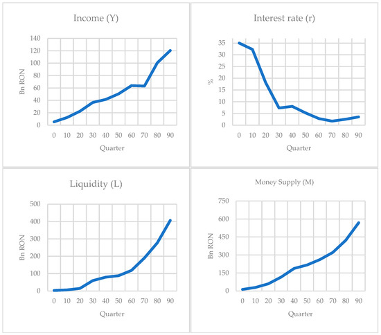
Figure 1.
Quarterly income , interest rate , liquidity (money demand) , and money supply in Romania, 2000Q1–2023Q2.
As shown in Figure 1, Romania’s real income experienced robust growth in the early 2000s, a sharp contraction during the 2008–2009 global financial crisis, a recovery in the 2010s, and another dip in 2020 due to the COVID-19 pandemic, followed by a rebound. The interest rate exhibited a downward trend from high levels in the early 2000s to single digits by the 2010s, reflecting disinflation and monetary easing, with a recent uptick in the 2020s due to rising inflation. The liquidity variable (which depends on both and ) broadly increased over time, especially as interest rates fell and the economy grew, indicating higher money demand. The money supply also rose substantially, consistent with economic growth and monetisation of the economy. These trends provide context for calibrating our model’s initial conditions and verifying its output.
4.2. Parameter Estimation and Model Calibration
We estimate structural parameters for the investment and liquidity functions using ordinary least squares for the log-linearised investment function and nonlinear least squares for the liquidity function.
Table 1 summarises the results of the log-linear OLS regression model estimating the determinants of public investment. The overall model was statistically significant, F(2, 92) = 159.7, p < 0.001, and explained approximately 77.6% of the variability in the dependent variable (ln I(n)), as indicated by an R2 of 0.776.

Table 1.
Estimated parameters of the public investment function (log-linear OLS).
The constant term () was estimated at −6.6625, corresponding to an implied value of approximately 0.0013 (), indicating a small baseline level of investment. The coefficient , representing output elasticity of investment, was significantly greater than one, suggesting strong accelerator effects—investment responds more than proportionally to changes in output. The positive estimate of implies a negative relationship between investment and interest rates due to the inverse log-linear specification (investment responds negatively to through the term ).
Table 2 presents the results of the nonlinear least squares estimation for the liquidity demand function. The model demonstrates a strong fit with a pseudo-R2 value of approximately 0.96, indicating that the specified model accounts for about 96% of the variability in liquidity demand. The residual sum of squares was 1.065 × 10¹¹, with a mean squared error of 1.115 × 10⁹.
Table 2.
Estimated parameters of the liquidity demand function (nonlinear least squares).
The large value of indicates that the transaction motive, linked to income, constitutes the primary driver of liquidity demand. While is small and statistically insignificant (p = 0.803), the high estimate of (≈2.88) reveals strong nonlinear sensitivity of speculative demand to changes in interest rates. As interest rates approach zero, the expression increases sharply, reflecting a surge in liquidity demand, consistent with Keynesian liquidity preference theory, which predicts increased money demand when interest rates are low.
Using these estimates, we calibrate other model parameters based on observed averages or reasonable assumptions (Table 3):
Table 3.
Calibration of additional model parameters.
The effective tax rate is set at reflecting Romani’s average tax-to-GDP ratio of approximately 16.67% over the 2000–2023 period (World Bank, n.d.). This value also aligns with the statutory flat tax rate of 16% on both personal and corporate income that was in place from 2005 until the 2017 tax reform, after which the personal income tax was reduced to 10%. Compared to international benchmarks, this figure is significantly lower than the OECD average tax-to-GDP ratio of approximately 33.9% (OECD, 2024) and the EU average of around 40% (Eurostat, 2024). This divergence highlights Romania’s more limited fiscal capacity and helps explain the choice of a lower tax parameter in our calibration. By using 16% as a stylised proportional tax rate on income, we ensure empirical consistency with national fiscal structure while maintaining model tractability in the context of emerging-market dynamics. The output adjustment speed parameter implies that approximately 150% of the output gap is closed per period, allowing the model to respond dynamically while avoiding excessive oscillations. This moderate adjustment speed strikes a balance between responsiveness and stability, and will be further explored during bifurcation analysis. The interest rate adjustment speed is set deliberately low to reflect central bank smoothing behaviour—interest rates do not adjust instantly to market disequilibria, which mirrors real-world monetary policy inertia. The money supply adjustment speed reflects a relatively fast convergence process. In this specification, the money stock catches up to income dynamics within a few quarters, ensuring rapid monetary feedback in response to real activity. The memory decay parameter governs the exponential weighting applied to past incomes. This value implies relatively slow memory decay, acknowledging that agents’ expectations and behaviour respond not only to current but also recent past income levels. In some simulations, a discrete memory alternative (e.g., fixed lag or distributed delay) is also examined for comparison. Government spending is treated as an exogenous input, updated per simulation period using actual historical data.
5. Results
Using the calibrated model parameters, we investigate the dynamic behaviour of the economy under two distinct fiscal policy regimes: one with instantaneous tax collection and one with a delayed tax response.
Variant 1 (immediate taxation) assumes that taxes are collected with no delay, i.e., each period. This corresponds to setting in the model (no memory in taxation).
Variant 2 (delayed taxation) bases tax collection on a weighted history of past income, introducing a discrete memory form with and (a two-year lag component). Thus depends partly on income from 2 years ago. This introduces a substantial delay in the fiscal feedback.
We initialise all the simulations at empirically observed 2000 values for key variables (, , and ), ensuring both variants start from the same baseline. The model is then iterated forward in discrete time to examine how each taxation scheme influences the paths of income, interest rate, and money supply. In the absence of exogenous shocks, Variant 1 is expected to converge to equilibrium given its alignment with the standard IS–LM stability conditions, whereas Variant 2 introduces the potential for persistent fluctuations due to the feedback lag.
To systematically explore how the output adjustment speed affects the model’s dynamics under each taxation regime, we conduct a bifurcation analysis. The parameter governs how aggressively outputs , , and react each period to an excess demand (IS imbalance)—a low means the economy corrects slowly, whereas a high implies a rapid (potentially overshooting) response. In conventional linear models without delays, increasing typically hastens convergence until extreme values, where instability might occur. However, in the presence of delays, even moderate increases in can fundamentally alter stability.
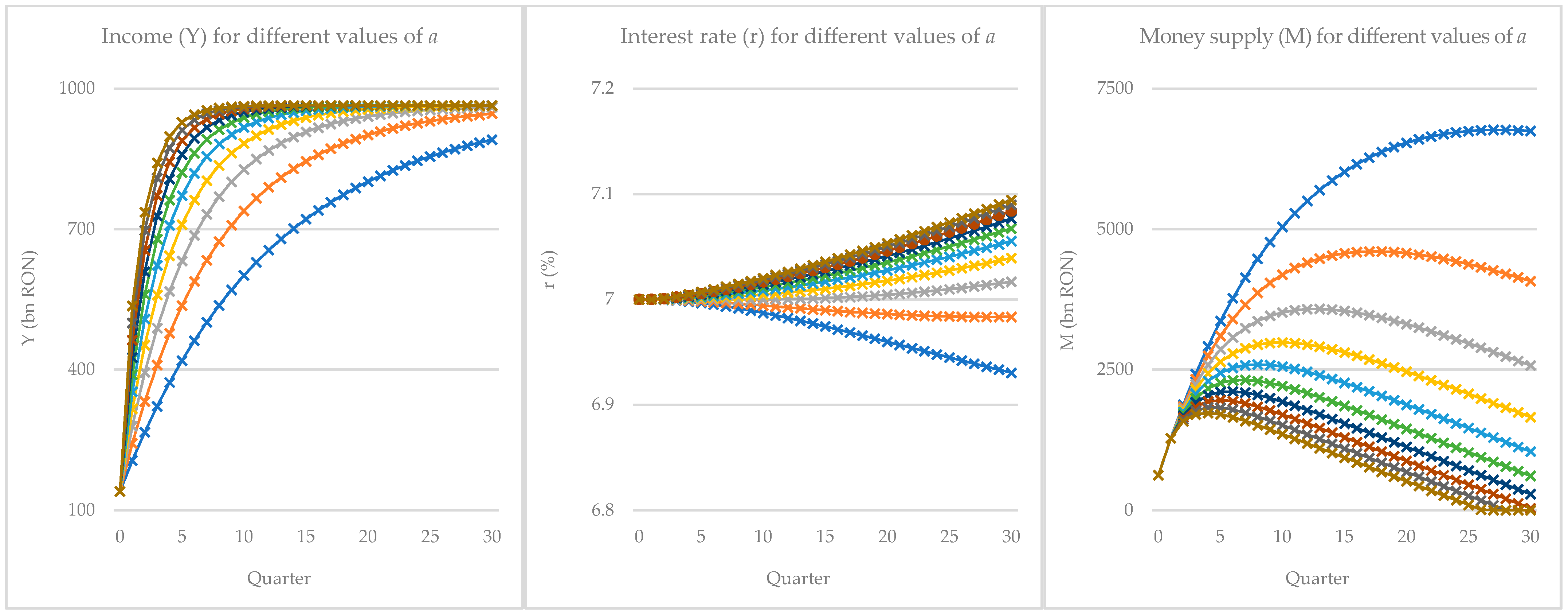
In our numerical simulation, the immediate-taxation case remains stable for all the tested values of in a substantial range (we examined from up to , which far exceeds typical empirical estimates for output adjustment speeds). Figure 2 illustrates dynamic trajectories of , , and over 30 periods for ten sample values of in this range. All trajectories converge to the same equilibrium without oscillations. As increases, the speed of convergence increases as well—higher drives a faster initial jump toward equilibrium values—but importantly, no cyclical or divergent behaviour emerges. Even at (the upper end of the considered range), the system simply settles more quickly, underscoring a large stability margin in the absence of fiscal delays. These results suggest that with immediate fiscal feedback, the model’s equilibrium is globally or at least locally asymptotically stable for a wide parameter space. In technical terms, no bifurcation (neither a flip/period-doubling nor a Hopf bifurcation) is detected for within the tested interval under Variant 1. The Jacobian eigenvalues remain inside the unit circle (discrete time case) or have negative real parts (continuous-time analogy), reflecting a well-damped system. This robustness aligns with the classical stability results for IS-LM models and resonates with earlier findings that straightforward fiscal rules can stabilise output as long as they respond without delay (Liao et al., 2005). In essence, immediate taxation acts akin to an active feedback control that continuously dampens fluctuations.

Figure 2.
(Immediate Taxation)—dynamic trajectories of income (), interest rate (), and money supply () over 30 periods with no tax delay. Ten values of the adjustment speed in are shown. Higher shortens the time to equilibrium but does not induce oscillations or instability. All the variables monotonically approach their steady-state values, indicating strong stability under prompt taxation.
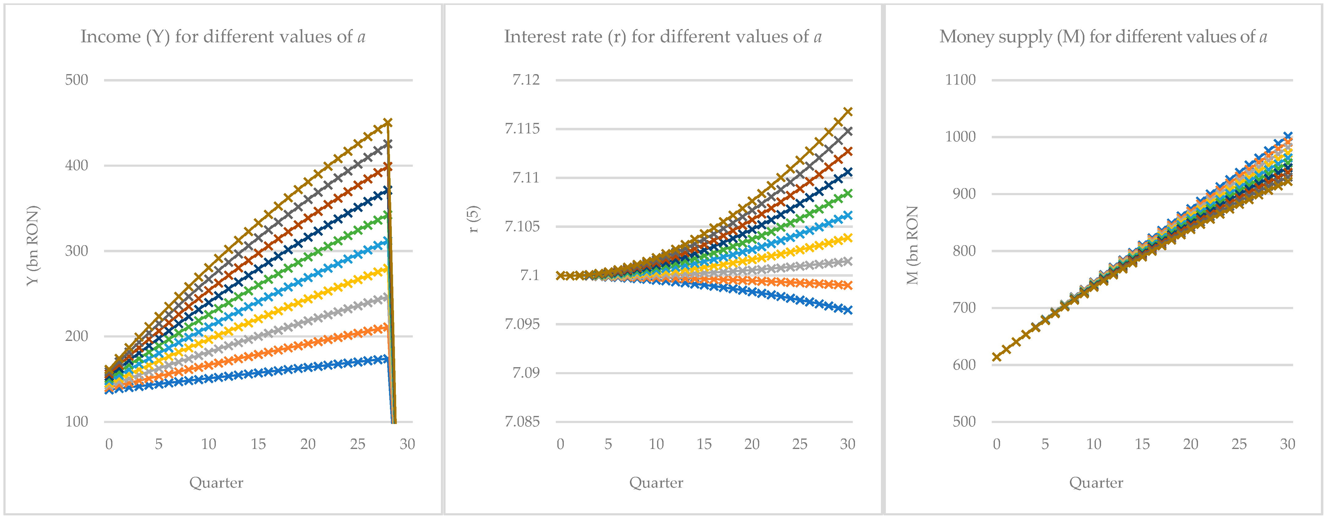
On the other hand, the delayed-taxation regime reveals signs of dynamic instability as the adjustment speed parameter increases. Figure 3 presents the simulated trajectories of income (), interest rate (), and money supply () over 30 quarters, for ten values of , under a discrete-time IS-LM framework with a two-period tax collection delay.
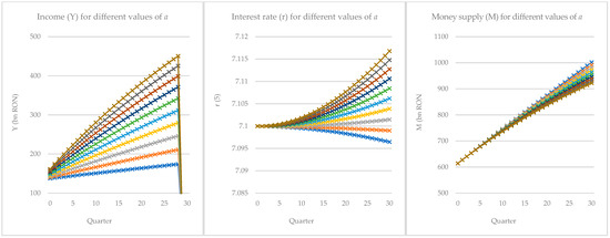
Figure 3.
(Delayed Taxation)—simulated trajectories of , , and over 30 periods with a two-year tax collection lag (Variant 2). Ten values of in [0.5, 3] are shown. Initially, higher leads to faster growth in , but as approaches 3, the system exhibits a nonlinear breakdown in income by period 30, indicating loss of stability. Interest rate and money supply paths remain smooth in the short run, but the long-run equilibrium for ceases to be attainable, signalling a bifurcation-induced regime shift.
At lower values of (e.g., ), the economy converges smoothly toward a stable equilibrium. As increases, income grows more rapidly in the early periods, reflecting a stronger adjustment response to demand shocks. However, for values of exceeding approximately 2.8, a marked change in system behaviour emerges. The income paths exhibit increasingly steep growth followed by a sudden collapse in the final simulation period. This collapse, observed for the highest values of , is not preceded by visible oscillations within the simulation window, suggesting an abrupt loss of stability rather than a gradual transition via damped cycles.
This pattern is indicative of a Neimark–Sacker bifurcation, in which a pair of complex-conjugate eigenvalues of the Jacobian cross the unit circle, causing the steady state to lose stability and giving rise to cyclical or quasi-periodic behaviour. Although no full cycle is formed within the 30-period horizon, the final-period crash in output is consistent with the trajectory departing from the equilibrium orbit as a result of delayed feedback dynamics. The interest rate () and money supply () remain relatively well-behaved across all values of , exhibiting monotonic or gently increasing paths. This is due to their structurally inertial responses and the presence of exogenous influences in the monetary equation. While both variables are indirectly affected by output instability, they do not collapse in tandem with income, further supporting the interpretation that it is the feedback delay in fiscal policy that destabilises the income path specifically.
The results of our numerical bifurcation analysis indicate that in the delayed taxation regime, higher values of the adjustment parameter substantially increase the risk of the system transitioning into complex or chaotic regimes.
The contrasting behaviour observed across the two taxation regimes underscores the critical role of timing in fiscal policy feedback. Under immediate taxation, the system consistently displays strong stability across the entire tested range of the adjustment speed parameter . Higher values of merely accelerate convergence to equilibrium without inducing any oscillatory or divergent behaviour. This robust performance aligns with theoretical expectations from classical IS–LM dynamics, where prompt feedback acts as a stabilising force, effectively damping excess demand and preventing cyclical amplification.
By contrast, the delayed-taxation regime introduces a structural vulnerability. Although the system initially tracks a similar growth trajectory, the delayed feedback loop begins to interact nonlinearly with the increasing adjustment speed. As approaches the upper bound of the tested range, the simulations reveal an abrupt and pronounced collapse in output, a sharp deviation from the otherwise monotonic convergence observed in the immediate-taxation case. This breakdown, appearing without visible precursors such as damped oscillations, suggests the presence of a bifurcation threshold beyond which the system loses local stability.
The income collapse observed at high values of under delayed taxation is consistent with the onset of a Neimark–Sacker bifurcation, a mechanism through which stability is lost as complex-conjugate eigenvalues of the system’s Jacobian cross the unit circle. Although full-cycle behaviour does not develop within the simulation window, the sharp deviation at the end of the horizon indicates that the model is departing from the equilibrium manifold and transitioning toward a new, possibly quasi-periodic or unstable regime.
These findings reinforce the central insight that fiscal lags can severely constrain the stability region of macroeconomic adjustment. In the presence of delayed taxation, even moderate increases in the speed of adjustment, typically considered beneficial in reducing output gaps, can lead to unintended destabilising effects. In practical terms, this implies that not only the strength but also the responsiveness of fiscal mechanisms matter for macroeconomic stability. While immediate feedback allows for aggressive policy action without sacrificing equilibrium, delayed feedback amplifies the risk of instability and constrains the effectiveness of otherwise sound policies. Our findings are consistent with prior theoretical work on delayed feedback in macroeconomic systems. For instance, Neamtu et al. (2009) demonstrated that the introduction of taxation lags in discrete-time IS–LM models leads to Neimark–Sacker bifurcations at values of that would otherwise preserve stability in the absence of delay. Similarly, Liao et al. (2005) showed that extended policy lags in dynamic control models can induce Hopf bifurcations and transition the system toward complex or chaotic dynamics. Our contribution extends these insights by embedding the analysis within a calibrated IS–LM framework tailored to the Romanian economy, and by empirically illustrating how fiscal delays critically reduce the parameter region in which stable equilibria can be maintained.
6. Conclusions
This study presented an enhanced IS–LM macroeconomic model that explicitly incorporates fiscal delays and memory effects, offering new insights into how the timing of taxation influences economic stability. We formulated the model in both continuous and discrete time, with a focus on the tractable discrete version calibrated to Romania’s post-2000 data. The calibration and simulation exercise allowed us to validate the model’s qualitative behaviour against real-world patterns and to conduct controlled experiments on policy timing. Several key conclusions emerge from the analysis.
First, the contrast between the immediate and delayed taxation regimes underscores the critical importance of policy timing in maintaining macroeconomic stability. With immediate taxation (fiscal policy responding within the period to income changes), the model economy dampens fluctuations and maintains stability even when the system is otherwise quite reactive. In this regime, higher adjustment speeds accelerate the return to equilibrium rather than cause instability. By comparison, delayed taxation can serve as an intrinsic source of instability. We observed that introducing realistic lags in tax collection generated endogenous cycles and even chaotic dynamics at parameter values that would be entirely stable under an immediate collection regime. The policy implication is clear: governments should strive to minimise unnecessary lags in fiscal interventions. Rapid adjustments of taxes and spending (for example, via well-designed automatic stabilisers that move in phase with the economy) act to stabilise output, whereas policies that respond too slowly (retrospective or lagged fiscal rules) may unintentionally amplify volatility.
In practical terms, reducing fiscal delays is not only desirable but increasingly feasible. Advances in tax administration, real-time reporting, and digital infrastructure offer governments the technical means to reduce the lag between income generation and fiscal response. However, institutional inertia, legislative rigidity, and budgeting cycles often impede rapid adjustments. While assertive fiscal responses can help close output gaps, our findings caution that in the presence of delays, greater responsiveness may lead to instability. A practical policy alternative lies in the use of automatic stabilisers, rules that adjust tax rates or public spending based on real-time indicators such as output or employment. These stabilisers can provide counter-cyclical force without requiring delayed political action, and their proper design should account for the presence of memory effects to avoid exacerbating volatility.
Second, by introducing a memory-dependent income variable, our model captures how past economic conditions exert a persistent influence on current outcomes. This feature proved useful in explaining real-world phenomena such as prolonged booms and busts that cannot be captured by memory-less models. For instance, Romania’s post-2008 recession and the prolonged recovery that followed can be partially explained by persistent structural rigidities and delayed policy response—dynamics that are effectively captured by the memory structure embedded in our model. The memory formulation improved the model’s ability to track actual data patterns, such as the lag between an output shock and the corresponding fiscal strain (e.g., tax revenue shortfalls and delayed budget adjustments). This underscores that policy measures (like budgeting based on past revenue) and private behaviours (habit formation in consumption, or firms’ investment plans based on past demand) create inertia in the economy. Policymakers need to account for this inertia: a one-off stimulus or austerity measure may have delayed effects and can lead to unintended oscillations if not monitored over time. In sum, incorporating economic memory provides a richer understanding of how history matters in macroeconomics, echoing the insights from recursive models in which expectations and past states jointly determine current equilibrium.
Third, our analysis demonstrates that the economy can undergo qualitative regime changes when structural parameters cross certain thresholds. In particular, making the system more reactive (e.g., a larger due to aggressive investment responses or pro-active fiscal policy) can push the system from a stable regime into a cyclic or chaotic regime if a delay is present. This highlights the limitations of purely linear intuition in macroeconomics. Traditional linear models might suggest that “more responsiveness is always better” for correction, but our results show a caveat: beyond a point, increased sensitivity in a system with delays leads to instability. This is analogous to findings in other nonlinear business cycle models (e.g., the classic multiplier-accelerator model of Samuelson, which can produce cycles when parameters are in certain ranges). For policymakers, this means that pushing policy aggressiveness beyond a threshold can backfire if the policy process is not nimble. Near those critical thresholds, the economy can exhibit large boom–bust cycles from even small disturbances. Thus, understanding the system’s nonlinear responses is important for designing policies that are effective but still keep the economy in a stable regime.
Fourth, the findings reinforce the idea that effective macroeconomic management must consider not just the size of fiscal interventions, but also their timing and feedback properties. A policy rule that looks forward (or at least contemporaneously) is likely to outperform one that looks backwards in terms of stability. A possible extension of fiscal policy could be to index tax rates to current or expected near-future incomes, thereby neutralising the memory effect by anticipating the cycle rather than reacting to the last cycle. In practice, this could involve more frequent tax adjustments or counter-cyclical fiscal rules that trigger based on real-time indicators. In economies where fiscal lags are unavoidable, other stabilisation mechanisms, such as more active monetary policy or macroprudential tools, should be strengthened to counterbalance the delay-induced cycles. Our model offers quantitative insights that otherwise minor frictions, like a few-period fiscal delay, can significantly destabilise outcomes, underscoring the value of coordinated and responsive macroeconomic governance.
Finally, by calibrating our model to two decades of Romanian data, we showed that the enriched IS–LM framework can replicate key patterns of macroeconomic fluctuations observed in the real world. The model tracked the general trajectory of Romania’s economy, capturing the growth of the early 2000s, the significant downturn during 2008–2009, and the subsequent oscillations during recovery better than a memory-less model could. This validation builds confidence that incorporating fiscal delays and memory effects is not only theoretically significant but also empirically relevant. The framework can be used for scenario analysis and stress-testing. Policymakers in Romania or similar emerging markets might simulate, for instance, how a delay in implementing a new tax policy could affect economic volatility, or how quickly a stimulus should be withdrawn after a recession to avoid undesired cycles. Extensions could include external sectors, inflation dynamics, or optimal policy rules under memory, enhancing its usefulness for decision-making.
That said, the current model does not include external shocks or open-economy setting features, particularly relevant for Romania as a European Union member with significant trade and capital flow exposure. The exclusion of exchange rates, inflation, and monetary spillovers limits the model’s ability to assess international policy coordination or currency-related vulnerabilities. Nonetheless, the simulations provide valuable insights for domestic fiscal governance. Romania’s recurring deficit challenges and administrative delays in implementing tax policies mirror the destabilising effects predicted by the model’s delayed taxation regime. The findings suggest that reducing fiscal inertia by streamlining tax collection processes, deploying automatic stabilisers, and enhancing real-time monitoring could help mitigate endogenous cycles and long recovery periods. Future work could extend the framework to include an external sector, stochastic disturbances, and price-level effects, allowing for broader scenario analysis under conditions of uncertainty and international interdependence.
This work bridges theoretical and empirical analysis to demonstrate that when and how fiscal policy is implemented can be as important as the policy itself. By extending the classical IS–LM paradigm to include realistic features like delayed taxation and adaptive expectations (memory), we uncovered mechanisms through which policy lags can destabilise the economy. The enhanced model offers a richer lens for understanding macroeconomic stability and provides actionable insights: to achieve stable and sustainable growth, policymakers should design fiscal rules that either avoid significant delays or are complemented by other measures to counteract the destabilising effects of those delays.
Author Contributions
Conceptualisation, C.P. and S.B.; methodology, C.P., S.B. and L.J.; resources, L.J.; writing—original draft preparation, L.J.; writing—review and editing, C.P., S.B. and L.J. All authors have read and agreed to the published version of the manuscript.
Funding
This research received no external funding.
Institutional Review Board Statement
Not applicable.
Informed Consent Statement
Not applicable.
Data Availability Statement
The data used in this study are publicly available at the Romanian National Institute of Statistics and the Romanian National Bank.
Conflicts of Interest
The authors declare no conflicts of interest.
References
- Barro, R. J. (1990). Government spending in a simple model of endogeneous growth. Journal of Political Economy, 98(5), S103–S125. [Google Scholar] [CrossRef]
- Blanchard, O. J., & Kahn, C. M. (1980). The solution of linear difference models under rational expectations. Econometrica: Journal of the Econometric Society, 48, 1305–1311. [Google Scholar] [CrossRef]
- Bracewell, R. N., Cherry, C., Gibbons, J. F., Harman, W. W., Heffner, H., Herold, E. W., Linvill, J. G., Ramo, S., & Rohrer, R. A. (2000). McGraw-hill seires in electrical and computer engineering. In The fourier transform and its applications. McGraw Hill Boston. [Google Scholar]
- Cai, J. (2005). Hopf bifurcation in the IS-LM business cycle model with time delay. Electronic Journal of Differential Equations (EJDE)[electronic only], 2005, 1–6. [Google Scholar]
- Christiano, L. J., Eichenbaum, M., & Evans, C. L. (2005). Nominal rigidities and the dynamic effects of a shock to monetary policy. Journal of Political Economy, 113(1), 1–45. [Google Scholar] [CrossRef]
- Cox, D. R., & Lewis, P. A. W. (1966). The statistical analysis of series of events. Springer. (Epub ahead of print 1966). [Google Scholar]
- Eurostat. (2024). EU and euro area tax-to-GDP ratio down in 2023. [News release] European Commission. Available online: https://ec.europa.eu/eurostat/web/products-eurostat-news/w/ddn-20241031-1 (accessed on 10 July 2025).
- Fisher, D., & Fisher, D. (1983). The investment function. In Macroeconomic theory: A survey (pp. 269–347). Springer. [Google Scholar]
- Hicks, J. R. (1937). Mr. Keynes and the” classics”; a suggested interpretation. Econometrica: Journal of the Econometric Society, 5, 147–159. [Google Scholar] [CrossRef]
- Kotz, S. (1970). Distributions in statistics: Continuous univariate distributions. John Wiley & Sons. [Google Scholar]
- Liao, X., Li, C., & Zhou, S. (2005). Hopf bifurcation and chaos in macroeconomic models with policy lag. Chaos, Solitons & Fractals, 25(1), 91–108. [Google Scholar]
- Ljungqvist, L., & Sargent, T. J. (2018). Recursive macroeconomic theory. MIT Press. [Google Scholar]
- Mankiw, N. G., & Weinzierl, M. (2010). The optimal taxation of height: A case study of utilitarian income redistribution. American Economic Journal: Economic Policy, 2(1), 155–176. [Google Scholar] [CrossRef]
- McKenzie, L. W. (1989). General equilibrium. In General equilibrium (pp. 1–35). Springer. [Google Scholar]
- Modigliani, F. (1944). Liquidity preference and the theory of interest and money. Econometrica, Journal of the Econometric Society, 12, 45–88. [Google Scholar] [CrossRef]
- Neamtu, M., Mircea, G., Opris, D., & Mastorakis, N. E. (2009). A discrete IS-LM model with tax revenues. In WSEAS international conference. Proceedings. Recent advances in computer engineering. WSEAS. [Google Scholar]
- Neamţu, M., Opriş, D., & Chilarescu, C. (2007). Hopf bifurcation in a dynamic IS–LM model with time delay. Chaos, Solitons & Fractals, 34(2), 519–530. [Google Scholar]
- OECD. (2024). Revenue statistics 2024: Health taxes in OECD countries. OECD Publishing. Available online: https://www.oecd.org/en/publications/revenue-statistics-2024_c87a3da5-en.html (accessed on 10 July 2025).
- Ross, S. M. (2014). Introduction to probability models. Academic Press. [Google Scholar]
- Saez, E. (2001). Using elasticities to derive optimal income tax rates. The Review of Economic Studies, 68(1), 205–229. [Google Scholar] [CrossRef]
- Schwartz, L. (1950). Théorie des distributions. I, II (Hermann et Cie, Paris) Math. Rev, 12, 31. [Google Scholar]
- Smets, F., & Wouters, R. (2007). Shocks and frictions in US business cycles: A Bayesian DSGE approach. American Economic Review, 97(3), 586–606. [Google Scholar] [CrossRef]
- Tijms, H. C. (2003). A first course in stochastic models. John Wiley and sons. [Google Scholar]
- Tramontana, F., & Gardini, L. (2021). Revisiting Samuelson’s models, linear and nonlinear, stability conditions and oscillating dynamics. Journal of Economic Structures, 10, 9. [Google Scholar] [CrossRef]
- Woodford, M. (2011). Simple analytics of the government expenditure multiplier. American Economic Journal: Macroeconomics, 3(1), 1–35. [Google Scholar] [CrossRef]
- World Bank. (n.d.). Tax revenue (% of GDP)—Romania [Data set]. Available online: https://data.worldbank.org/indicator/GC.TAX.TOTL.GD.ZS?locations=RO (accessed on 6 April 2025).
Disclaimer/Publisher’s Note: The statements, opinions and data contained in all publications are solely those of the individual author(s) and contributor(s) and not of MDPI and/or the editor(s). MDPI and/or the editor(s) disclaim responsibility for any injury to people or property resulting from any ideas, methods, instructions or products referred to in the content. |
© 2025 by the authors. Licensee MDPI, Basel, Switzerland. This article is an open access article distributed under the terms and conditions of the Creative Commons Attribution (CC BY) license (https://creativecommons.org/licenses/by/4.0/).