The Role of Sequencing Economics in Agglomeration: A Contrast with Tinbergen’s Rule

Abstract

In this paper, we present the concept of “sequencing economics”, consisting of (A) segmentation, (B) construction sequencing, and (C) functions. An agglomeration is organized into segments, and sequencing economics examines the sequential process of efficiently building such segments. The functions (C) of the segments act as a master switch, an accelerator, a brake, etc. in the implementation of agglomeration policy. In this paper, we identify a master switch and an accelerator in scientific city agglomeration policy and draw two conclusions. First, in agglomeration policy, the construction of the master switch lowers “transport costs”, as derived from the monocentric city model of spatial economics by Fujita and Krugman. Second, the accelerator segment represents the activities of the service sector that have the highest forward-linkage effect in an input–output relationship. Regarding science city agglomeration policy, it can be concluded that the master switch is high-speed rail and the accelerator is research and education activities. In this paper, the new scientific urban agglomeration that emerges from monocentric cities is referred to as railroad-driven agglomeration (RDA), which is a type of transit-oriented development (TOD). This paper demonstrates that the Tsukuba Express, as a case study of RDA, caused the agglomeration of Tsukuba Science City. This paper establishes the concept of sequencing economics, a policy implementation rule that differs from Tinbergen’s rule. The latter is based on the concept of simultaneous equations, whereas the rule of sequencing economics is based on sequential equations. RDA enables middle-income countries to surpass their middle-income status.

1. Introduction

JICA (2014) projected that the ASEAN region will not escape “the middle-income trap” by 2025. According to the World Development Report (2024), 108 countries that have tackled poverty and climate change and have elevated themselves into a higher-income bracket were classed as middle-income countries at the end of 2023. These countries account for approximately 75% of the world’s population and 40% of the world’s GDP. The report recommends a change of gears, and employing strategic “innovation” to combine investment with infusion and innovation to escape the middle-income trap.

One of the prerequisites for this is “agglomeration.” Porter (1998) argued that the agglomeration of geographically proximate related industries promotes competitiveness and innovation. Audretsch and Feldman (1996) concluded that corporate R&D activities generate externalities (spillovers) through urban agglomeration, thereby enhancing regional innovation. We examine agglomeration as a device to generate an “innovation” strategy.

Calthorpe and like-minded New Urbanists argue that access to rail transit played a pivotal role in the development of urban living (Calthorpe, 1993; Calthorpe Associates, 1992). The agglomeration design concept of “transit-oriented development (TOD)” extended the land use and transportation nexus.

However, the TOD approach has not been linked to agglomeration analysis in sequencing economics to identify a “master switch” for the agglomeration of TOD, nor has it been linked to spatial economics in order to specify the function of the master switch for practical policy. We focus on a scientific urban agglomeration that emerges from a “monocentric city” as railroad-driven agglomeration (RDA), a type of transit-oriented development (TOD).

We present the concept of “sequencing economics”, which establishes sequences for the efficient construction of the segments of an agglomeration. Sequencing economics analyzes the (C) function of segments and identifies the master switch, accelerator, and brake in the segment construction process. Taylor (1911), known as the father of “Scientific Management”, advocated efficient management in construction projects. Scientific management is defined as (A) segmentation and (B) construction sequencing from the perspective of the construction industry, as shown in

Table 1. Sequencing economics.

Economics	(A) Segmentation, (B) Construction Sequencing	(C) Segment Function
Characteristics	(A) Segments	(C) Functions
Key Segments	Residential town, public spaces, airports, factories, IT OS and data center business, and so on	(C) (i) Master switch, (ii) Accelerator, (iii) Brake
Theory	Scientific management: CPM, PERT, BIM etc.	Flowchart Approach: economies of sequence
Source	Taylor (1911), Gantt (1910)	Kuchiki (2024a), Kuchiki (2023), Kuchiki and Sakai (2023)

Note: CPM (critical path method), PERT (program evaluation review technique), BIM (building information modeling), etc. Source: Compiled by the author.

.

Segments that are “master switches” in agglomeration formation are those that satisfy the “breaking condition” for equilibrium in spatial economics, as shown in

Table 2. Segment function in sequencing economics.

Types of Agglomerations	Function	Segment	Spatial Economics	Papers	Location
Urban agglomeration	(1) Master switch	Transport costs	Krugman (1991), Alonso (1964)	Kuchiki and Sakai (2023)	Sapporo, Japan
Manufacturing	(2) Accelerator	Industrial zones	Helpman and Krugman (1985)	Kuchiki (2023)	Industrial hubs, China
Manufacturing	(3) No braking	Engineers	Helpman and Krugman (1985)	Kuchiki (2024a)	Industrial hubs, India
Knowledge and manufacturing industry	(4) Start switch	Research funding	Fujita and Thisse (2003)	Kuchiki (2024b)	Nations
Scientific city	(1) Master switch	Transport costs	Fujita and Krugman (1995)	This paper	Tsukuba Science City

Source: Compiled by the author.

. The first, second, and third columns of Table 2 show the type, function, and segment of agglomeration in sequencing economics. The master switch for urban agglomeration policy according to Kuchiki and Sakai (2023) is the “transport segment”.

The purpose of this paper is to identify the master switch and the accelerator in the policy of scientific city agglomeration. The following three steps are taken. First, we propose two hypotheses: Hypothesis 1: A master switch for an urban agglomeration policy is the construction of a segment that lowers “transport costs”, using Fujita and Krugman’s (1995) equilibrium condition of monocentric cities as “breaking conditions”. Hypothesis 2: An accelerator is the activity of “research and education” in the service sector that has the highest forward-linkage effect in the input–output relationship. We confirm that the forward-linkage effect of research and education in the service sector is the highest among all sectors, using the Asian International Input–Output Table 2000 compiled by the Institute of Developing Economies-JETRO (2006).

Regarding Hypothesis 1, we examine the case of Tsukuba Science City agglomeration in Japan using the Granger causality, together with the cases of the Hankyu Corporation and Odakyu Corporation in Japan, to illustrate RDA.

We conclude that, regarding science city agglomeration policy, the master switch is high-speed rail, and the accelerator is research and education activities.

This paper contributes to the establishment of “sequencing economics” with regard to the segments of agglomeration. Sequencing economics is a “policy implementation rule” that differs from Tinbergen’s (1952) rule. While Tinbergen’s rule is based on the concept of simultaneous equations, the rules of sequencing economics are based on sequential equations.

This paper is organized as follows. Section 2 reviews the literature and explains the model by Fujita and Krugman (1995) in spatial economics, which was used to obtain Hypothesis 1 of this paper. Section 3 confirms Hypothesis 2. Section 4 presents the Hankyu Railroad model as the prototype example of railroad-driven agglomeration (RDA), based on the Kobayashi Ichizo model. Section 5 identifies that a master switch for scientific city agglomeration is low-cost railroad transport in the case of Tsukuba Science City. Section 6 concludes the paper.

2. Spatial Economics Approach to Railroad-Driven Agglomeration (RDA)

2.1. Literature Review

This subsection reviews (i) Tinbergen’s rule, (ii) sequencing, (iii) scientific management, (iv) sequencing economics, (v) transit-oriented agglomeration, and (vi) spatial economics, in this order.

2.1.1. Tinbergen’s Rule

Tinbergen’s (1952) rule is a “policy implementation rule” that differs from sequencing economics. Tinbergen’s rule is based on the concept of simultaneous equations, while the rule in sequencing economics is based on the concept of sequential equations. Regarding the relationship between the number of policy objectives and the number of policy measures, Tinbergen’s rule asserts that in order to achieve a specific number of independent policy objectives, at least the same number of independent policy measures are necessary. In other words, the Tinbergen rule is based on the concept of simultaneous equations. While this rule is applicable to macroeconomic and trade policies, it is not applicable to many policies, such as “agglomeration policy”, national security policy, and environmental policy. Therefore, we propose the rule of sequencing economics based on the concept of sequential equations. “Sequencing” is explained in the next subsection.

2.1.2. Sequencing

Regarding “sequencing”, Johnston and Sundararajan (1999) provided positive insights into the complexities and considerations involved in sequencing policy measures in the context of the World Bank (2024) and IMF’s involvement in economic reforms. Their work explored the analytical and operational aspects of sequencing financial sector reforms. Zalduendo (2005) examined the optimal sequencing of reforms affecting the impact of economic policy on growth. Rodrik (2007) discussed the sequencing argument, stating that “liberalization before the institutions are in place will destabilize the economy. Regarding “agglomeration policies”, Kuchiki and Tsuji (2008) proposed a three-stage model, specifically proposing the order in which segments are constructed.

2.1.3. Scientific Management

Scientific management has long been applied to project management in the construction industry. This subsection explains the chronological development process of this management method. It applies the concept of efficient project management in scientific management to the policy implementation process of agglomeration in sequencing economics. The policy implementation process of agglomeration is a segment construction process, which must be an efficient process.

Taylor (1911) described a scientific approach to improving the efficiency of work processes. He advocated for methods such as work segmentation, standardization, time studies, and motion studies. The Gantt Chart, named after Gantt (1910), became a critical tool in project management. The study by Kelley and Walker (1959) was an early foundational work discussing the concepts of “construction sequencing” and “segmentation”.

Accordingly, scientific management is defined as (A) segmentation and (B) construction sequencing from the perspective of the construction industry, where industrial agglomerations are composed of segments.

Malcolm et al. (1959) described the Program Evaluation Research Task project as an integrated, quantitative evaluation of progress to date and the likelihood of accomplishing the objectives of the Fleet Ballistic Missile Program. Golizadeh (2017) focused on developing a process model that integrates image segmentation techniques with building information modeling (BIM) to automate construction progress monitoring, highlighting the importance of process segmentation in modern construction. Kuchiki (2023) identified segments with respect to the organization of urban agglomerations and revealed that segments have (C) “functions”.

2.1.4. Sequencing Economics

In this paper, we establish the concept of “sequencing economics” with regard to the segments of agglomeration: (A) segmentation, (B) construction sequencing, and (C) functions. We note that each segment has its own function, playing the role of a (i) master switch, (ii) accelerator, or (iii) brake in urban agglomeration policy. In studies by Kuchiki (2023) and Kuchiki (2024a), the accelerators and brakes for manufacturing agglomeration are described as the segments of industrial parks and the shortage of engineers, respectively, as shown in Table 1. The start switch for innovation in the knowledge and manufacturing industries is the research funding segment in Kuchiki’s (2024b) work.

Sequencing economics provides a lens through which to discuss (C) the function of the segments of an agglomeration. In this section, we obtain Hypothesis 1, focusing on “master switch” for science city agglomeration policy.

2.1.5. Transit-Oriented Development (TOD)

One method of organizing urban agglomerations is train-oriented development (TOD). Jamme et al. (2019) summarized a twenty-five-year biography of the TOD concept and pointed out that, as cities around the world become increasingly crowded, diverse, congested, and polarized, and as new modes of mobility emerge, TOD remains a promising model of development for inclusive, equitable, and sustainable communities.

Historically, this approach was established through the following four steps. Firstly, Howard (1902) proposed the concept of the “garden city”, which balances urban and rural life and provides the benefits of both environments without the drawbacks. Secondly, Warner (1962) explored the transformative urban development that occurred in Boston in the late 19th century, focusing on the emergence of “streetcar suburbs”. Hilton and Due (1960) chronicled the development of the “interurban railroad”, the once-dominant mode of transportation that linked urban centers with surrounding rural areas and small towns in the early 20th century.

Thirdly, regarding railroad construction and cultural activities, Fogelson (1967) details how the development of interurban railroads in the Los Angeles area promoted not only interurban logistics and residential development, but also the interactions between “cultural activities”. Finally, Calthorpe (1993) integrated the above ideas and introduced the concept of transit-oriented development (TOD), which advocates for compact, walkable, mixed-use neighborhoods centered around public transportation.

In this paper, we focus on analyzing the formation process by building the segments of a science city agglomeration based on high-speed trains, which is one aspect of the broad concept of TOD. We refer to one type of TOD, which is limited to science city agglomerations, as railroad-driven agglomeration (RDA). “Railroad” emphasizes the role of express railroads in reducing travel time as a form of transit. “Driven” refers to the process of forming agglomeration and constructing segments. During the construction process, it is necessary to identify segments that function as master switches and accelerators. Additionally, agglomeration is not merely a form of development, but rather a process of constructing segments, defined as the spatial concentration of economic activity. The breaking conditions of agglomeration equilibrium during agglomeration formation in spatial economics are used as the conditions for “master switches”.

2.1.6. Spatial Economics

Spatial economics models derive equilibrium conditions and “equilibrium-breaking conditions”. As shown in Table 2, Krugman (1991), Helpman and Krugman (1985), Fujita and Thisse (2003), and Fujita and Krugman (1995) have described the models used to obtain the breaking conditions listed by Kuchiki and Sakai (2023), Kuchiki (2023), and Kuchiki (2024b), respectively. The breaking condition derived from the monocentric city model of spatial economics from the isolated city of von Thünen to its connected cities determines a segment that functions as a “master switch”.

Simply deriving equilibrium-breaking conditions does not initiate the policy implementation process. The first step of agglomeration policy implementation is identifying segments that satisfy the equilibrium-breaking conditions obtained in spatial economics, followed by constructing them. These identified segments are called master switches and play a role in the initial construction of an agglomeration.

This section focuses on the breaking conditions of a monocentric city equilibrium in spatial economics in order to identify the master switch.

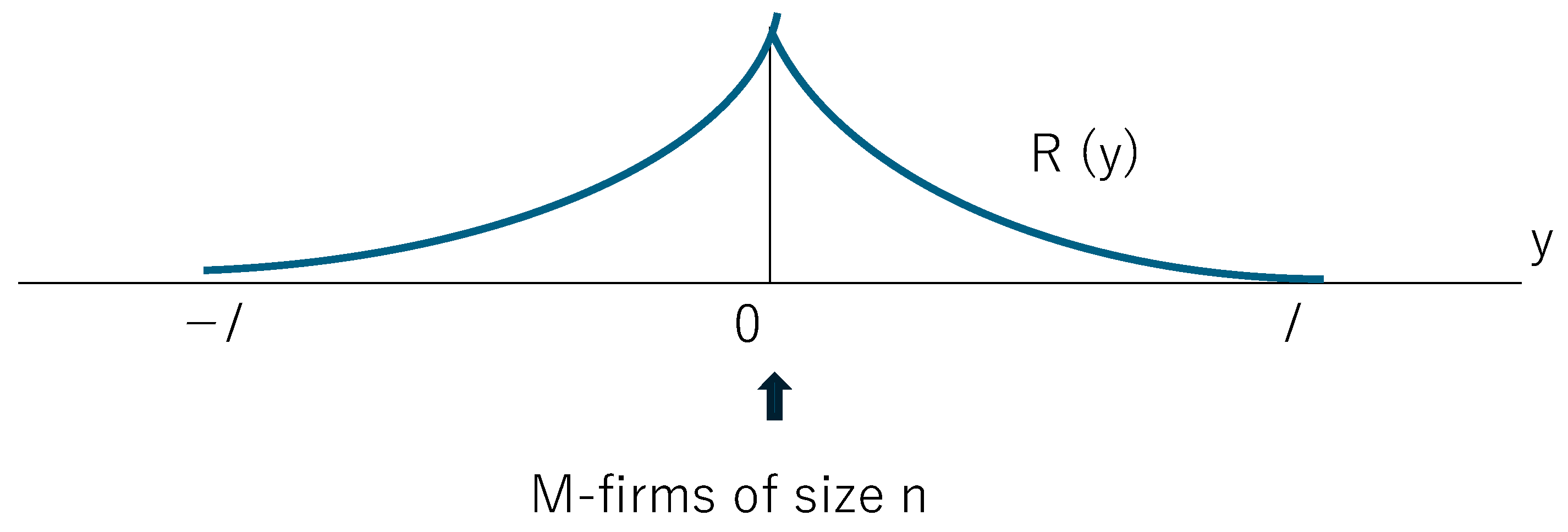
2.2. The Monocentric City Model of Fujita and Krugman

In this section, we reproduce the monocentric city model of Fujita and Krugman (1995), which focuses on the monocentric spatial configuration depicted in Figure 1.

All M-goods are assumed to be produced in a centrally located city, y = 0, and the agricultural area extends from −l to l. In the next section, we derive the conditions required for the emergence of new cities.

The economy has an agricultural sector (sector A: z) and a manufacturing sector (sector M: m), each supplying agricultural products and a continuum of differentiated manufacturing goods, respectively, to consumers. The quality of land is homogeneous, and the density of land is equal to 1 everywhere. Each worker is endowed with a unit of labor and is free to choose any location and job in the country. Consumers consist of workers and landlords. Workers’ income (Y) is earned from wages in the manufacturing sector (W). Every landlord is attached to their land and consumes the entire revenue generated from their land at their location.

Every consumer has the same utility function, given by

u = α_a ln z + α_m ln Q,

$$Q={[{\int }_0^{n}m\left(i\right)\mathsf{\rho }\mathrm{d}i]}^{1/\mathsf{\rho }},$$

(1)

where z represents the amount of A-goods, m(i) is the consumption of each variety, 0 ≦ i ≦ n of M-goods and services; and α_a, α_m, and ρ are positive constants, such that α_a + α_m = 1 and 0 < ρ < 1. The intensity of the preference for varieties in manufactured goods is expressed as σ and the elasticity of substitution between any two varieties is expressed as

σ ≡ 1/(1 − ρ).

Suppose that a consumer has an income, Y, and faces a set of prices, p_a for A-goods and p_m for M-goods. The budget constraint of a consumer is

$${\mathrm{p}}_{\mathrm{a}}\mathrm{z}+{\int }_0^n{\mathrm{p}}_{\mathrm{m}}\mathrm{m}(\mathrm{i})\mathrm{di}=\mathrm{Y}$$

Maximizing the utility function (1) subject to this budget constraint yields the following demand functions:

z = (α_a Y)/p_a,

(2)

m (i) = (α_m Y) p_m^−σ/G ^1−σ,

(3)

where G is the price index for M-goods, given by

$$G={[{\int }_0^n{p}_m{\left(i\right)}^{(1-\mathsf{\sigma })}\mathrm{d}i]}^{1/(1-\mathsf{\sigma })}.$$

Using the obtained functions (2) and (3), the indirect utility function can be obtained as follows:

$$u={\mathsf{\alpha }}_{\mathrm{a}}\ln {\mathsf{\alpha }}_{\mathrm{a}}+{\mathsf{\alpha }}_{\mathrm{m}}\ln \mathsf{\alpha }\mathrm{m}+\ln Y-{\mathsf{\alpha }}_{\mathrm{a}}\ln p_a-[({\mathsf{\alpha }}_{\mathrm{m}}/(\mathsf{\sigma }-1)]\ln [{\int }_0^n{p}_m{(i)}^{(1-\mathsf{\sigma })}\mathrm{d}i].$$

(4)

The production of A-goods is subject to Leontief technology, and each unit of A-goods consumes a unit of land and a_a units of labor. The total labor input, L, for the production of quantity Q of any product is given by

L = f + a_m Q,

where f is the labor requirement, and a_m represents the marginal labor input. The model by Fujita and Krugman (1995) assumes the ‘iceberg’ form of transport costs introduced by Samuelson. If Q is the output of the firm, its profit equals

π (x) = p_m (x) Q − W (x) (f + a_m Q) = a_m W (x) γ⁻¹(Q − γ f/a_m),

(5)

where γ ≡ ρ/(1 − ρ).

Therefore, given any equilibrium configuration of the economy, if an M-firm operates at x, then by the zero-profit condition of Equation (3), its equilibrium output is given by

Q* = γ f/a_m,

which is a constant independent of location.

The model by Fujita and Krugman (1995) assumes that the production of all M-goods takes place in the city located at the center, y = 0, and the agricultural area extends from −l to l. Therefore, this paper examines the location equilibrium conditions under which no M-firm deviates from the center city.

The price curve, p_a(y), of the A-goods is

p_a (y) = exp (−t_a |y|).

Next, the f.o.b. price (the mill price) of each M-good produced in the city is assumed to be

p_m = p_m (0). Therefore, the price of each M-good delivered at each location is given by

p_m (y) ≡ p_m (y|0) = p_m exp (t_m|y|).

Here, let W (y) be the equilibrium wage rate at each y ∈ [−l, l]. By definition, n is the number of firms producing M-goods in the city. The equilibrium wage rate at each y, W*(y), is given by

ln W*(y) = − ln a_a − exp α_m (t_m + t_a) l* + exp (α_m t_{m −} α_a t_a)|y|.

(6)

2.3. Relationship Between the Emergence of a New City and Lower Transport Costs

In this subsection, we obtain Hypothesis 1. Suppose that an M-firm is located at x. The price of the M-goods produced by the firm located at x and delivered (the c.i.f. price) to y is given by

p_m (y|x) = p_m (x) exp (t_m|y − x|) = a_m W*(x) ρ⁻¹ exp (t_m|y − x|).

The total demand for the firm located at x is obtained by

D (x, W*(x)) = [α_a γ f/(2 a_m)] (W*(0)/W*(x))^1+γ φ(x), for 0 ≦ x.

Using the equilibrium wage rate (6), the resulting firm’s profit is

π (x, W*(x)) = f W (x) (Ω (x) − 1),

where Ω (x) ≡ D (x, W*(x))/Q*.

The model by Fujita and Krugman (1995) calls Ω(x) the market potential function of the M-industry. Therefore,

Ω′ (0) ≡ dΩ(x)/dx | _x=0 = (1 + γ) [α_a t_a − (1 + ρ) α_m t_m].

(7)

(see Appendix A for the derivation of Equations (5)–(7) by Fujita and Krugman (1995)).

If [α_a t_a − (1 + ρ) α_m t_m] > 0, then Ω′ (0) > 0, resulting in Ω (x) > 1, and

π (x, W*(x)) > 0 = π (0, W*(0)).

The profit of the M-firm located at x is larger than zero, which is the profit of the M-firm located at 0. Fujita and Krugman (1995) found that a monocentric city cannot maintain equilibrium if [α_a t_a − (1 + ρ) α_m t_m] > 0 (see Table 1, p. 515), and supposed that, in this case, firms start operations in a new city at x from a monocentric city at 0.

In this paper, we derive the following condition:

∂Ω′ (0)/∂t_m = − (1 + γ) (1 + ρ) α_m < 0.

(8)

The sign of Equation (8) is negative. This means that the lower transport cost t_m is, the higher Ω′(0). The inequality of Ω(x) > 1 is realized by lowering transport costs. Hence, agglomeration policy starts with the construction of a segment that lowers transport costs. Therefore, we obtain the following hypothesis.

Hypothesis 1.

A master switch for urban agglomeration policy is the construction of a segment that lowers transport costs.

3. The Forward-Linkage Effects of the Sectors of Transport and Trade, and Services

In this section, we establish Hypothesis 2: An accelerator is the activity of “research and education” in the service sector that has the highest forward-linkage effect in the input–output relationship.

3.1. Tertiary Industries

According to the major economic categories, the economy consists of primary, secondary, and tertiary industries. Primary industries include agriculture and mining, while manufacturing is an example of a secondary industry.

Table 3. Tertiary industry activity.

Item_Number	Item_Name
J000000I	Tertiary Industry
JF00000I	Electricity, Gas, Heat Supply and Water
JG00000I	Information and Communications
JH00000I	Transport and Postal Activities
JI00000I	Wholesale and Retail Trade
JJ00000I	Finance and Insurance
JK00000I	Real Estate and Goods Rental and Leasing
JL00000I	Scientific Research, Professional and Technical Services
JM00000I	Accommodations, Eating and Drinking Services
JN00000I	Living-related and Personal Services and Amusement Services
JO00000I	Learning Support
JP00000I	Medical, Health Care and Welfare
JQ00000I	Compound Services
JR00000I	Miscellaneous Services (except Government Services etc.)
SBA0000I	Services
SBA1000I	Personal Services
SBA2000I	Business Services
SBB0000I	Broad-ranging Personal Services
SBB1000I	Broad-ranging Essential Personal Services
SBB2000I	Broad-ranging Non-essential Personal Services
SBC0000I	Broad-ranging Business Services
SBCB100I	Manufacturing-dependent Business Services
SBCB200I	Non-manufacturing-dependent Business Services
SBE2000I	Private Capital Investment Services
SBRA000I	Tourism Industry
SKEL000I	Tertiary Industry (except Wholesale and Retail Trade)

Source: Ministry of Economy, Trade and Industry of Japan (2024).

shows the tertiary industry subcategories, which include electricity, gas, heat supply and water, information and communications, wholesale and retail trade, finance and insurance, and other basic infrastructure necessary for daily life.

The transport and postal activities sector includes railroad transportation. Once “railroad transport” has been initiated and transport costs have been reduced, cultural activities cause the forward linkage of the input–output relationship. This paper examines various subsectors of cultural activities, including education and research (science) among others.

Stations that host “cultural activities”, such as sports stadiums, universities and research institutes, and theaters and museums, will be developed along the railroad lines. The tertiary sector of real estate and goods rental and leasing will enable the development of residential districts, which should have available accommodation, eating and drinking services, and medical treatment, healthcare, and welfare facilities. Thus, low-cost railroad transport will activate cultural activities.

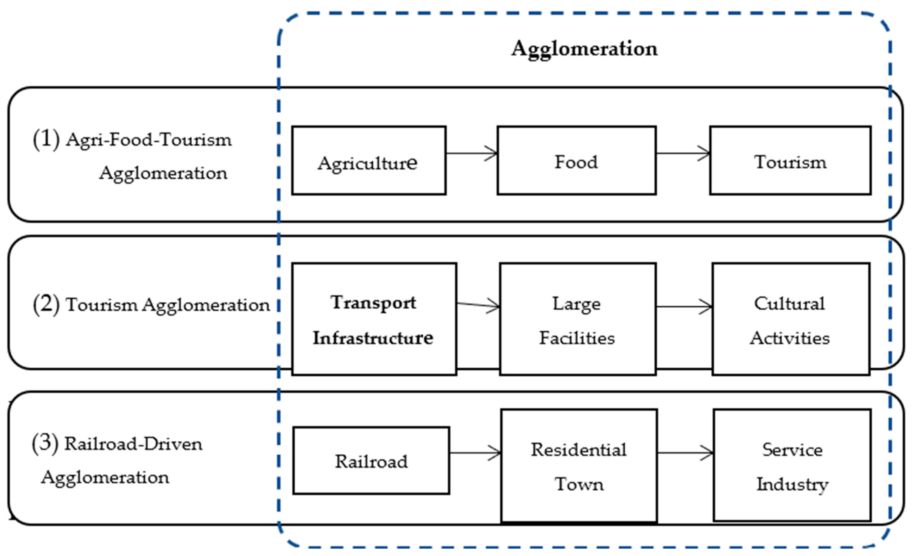
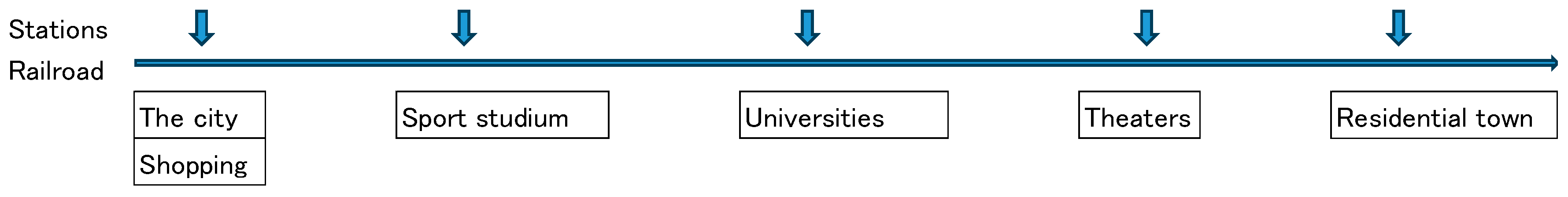
3.2. The Integration Model of Railroad Construction and Cultural Activities

The agricultural sector inputs the food manufacturing sector, which inputs the wholesale sector of the tertiary industry, which then inputs the retail sector, producing forward and backward industrial linkages.

Let us illustrate the case of an industrial linkage for a farm. As shown in Figure 2, the sequence encompasses the procurement of raw materials for production, the production of agricultural products, the processing of agricultural products, and the input to restaurants in the food service industry. The final output of these chains is in customers’ hands.

Figure 3 illustrates that the formation of agglomeration segments is associated with the development of primary, secondary, and tertiary (service) industries in the industrial agglomeration stage. The formation of agricultural, food, and tourism agglomerations is one of the measures implemented to improve the quality of consumption. Figure 3 hypothesizes that the segment formation sequence of railroad-driven agglomeration (RDS) involves the facilitation of railroad infrastructure, the construction of residential cities, and the emergence of scientific cities in the service sector.

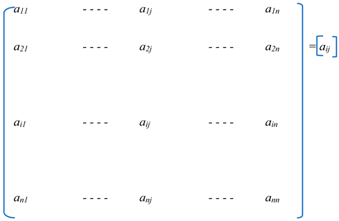
3.3. Definition of the Forward-Linkage Effect in the Input–Output Table

The technology coefficient (or input coefficient) in the input–output table is an indicator of the ratio of intermediate goods input from other industries to the output of an industry. The technology coefficient a_ij indicates how much of the input from industry i accounts for the total output of industry j. The input coefficient a_ij is defined as

a_ij = X_ij/X_i,

where

a_ij is the technology coefficient (or input coefficient) from industry i to industry j;

X_ij is the amount of intermediate goods input by industry j from industry I;

X_i is the total output of industry j.

The input coefficients of the input–output table are

Forward linkage in the context of an input–output table measures the extent to which a particular industry provides goods or services to other industries as inputs. It assesses the industry’s role as a supplier in the economy, highlighting how much its output influences downstream industries.

The effect of forward linkage in the input–output relationship is

$$\sum _{j=1}^n{a}_{ij}/{\displaystyle \frac{1}{n}}\sum _{i=1}^n\sum _{j=1}^n{a}_{ij}.$$

The Tsukuba Express opened in 2005. The analysis period for the Granger causality tests was from 2005 to 2019 (before the impact of COVID-19). The Asian International Input–Output Table 2000 by the Institute of Developing Economies-JETRO (2006) is available as a comparable international table for multi-country input–output tables close to 2005.

The table contains data from governments, central banks, and government-affiliated research institutes of Indonesia, Malaysia, the Philippines, Singapore, Thailand, China, Taiwan, Korea, Japan, and the United States.

Table 4. The average values of the effects of forward linkage in ten economies.

		Indonesia	Malaysia	Philippines	Singapore	Thailand	China	Taiwan	Republic of Korea	Japan	U.S.	The Average
1	Paddy	0.732	0.633	0.629	0.517	0.672	0.762	0.584	0.73	0.595	0.517	0.6371
2	Other agricultural products	0.902	0.896	0.741	0.567	0.92	1.263	0.8	0.592	0.624	1.009	0.8314
3	Livestock and poultry	0.609	0.721	0.606	0.519	0.628	0.771	0.803	0.676	0.642	0.787	0.6762
4	Forestry	0.698	0.8	0.556	0.517	0.559	0.698	0.521	0.578	0.651	0.838	0.6416
5	Fishery	0.564	0.61	0.559	0.519	0.642	0.626	0.673	0.566	0.576	0.524	0.5859
6	Crude petroleum and natural gas	1.813	1.158	0.519	0.517	0.81	1.274	0.559	0.517	0.523	1.071	0.8761
7	Other mining	1.096	0.61	0.662	0.558	0.637	1.074	0.605	0.615	0.592	0.723	0.7172
8	Food, beverage and tobacco	1.043	1.531	0.866	0.708	1.125	1.033	1.109	1.066	0.991	0.925	1.0397
9	Textile, leather, and the products thereof	0.803	0.692	0.653	0.615	0.839	1.733	0.992	0.968	0.871	0.824	0.899
10	Timber and wooden products	0.675	0.734	0.602	0.577	0.6	0.72	0.564	0.683	0.693	0.755	0.6603
11	Pulp, paper and printing	0.822	0.789	0.641	0.639	0.766	0.992	0.898	1.07	1.355	1.195	0.9167
12	Petroleum and petro products	1.008	1.049	0.791	0.962	0.986	2.475	1.498	2.148	2.734	2.034	1.5685
13	Other manufacturing products	0.808	1.268	1.119	1.37	1.141	1.583	0.911	1.361	0.983	1.006	1.155
14	Rubber products	0.584	0.587	0.58	0.552	0.677	0.744	0.585	0.606	0.707	0.604	0.6226
15	Non-metallic mineral products	0.591	0.75	0.678	0.617	0.7	0.858	0.734	0.787	0.812	0.706	0.7233
16	Metal products	0.818	0.998	0.833	0.801	0.77	2.137	1.262	1.79	2.648	1.522	1.3579
17	Machinery	0.711	0.952	0.63	0.804	0.919	2.15	1.184	1.373	2.757	1.832	1.3312
18	Transport equipment	0.893	0.744	0.538	0.702	0.809	1.177	0.765	0.853	1.627	0.94	0.9048
19	Other manufacturing products	0.593	0.798	0.594	0.816	0.722	1.108	0.783	0.893	1.367	1.052	0.8726
20	Electricith, gas, and water supply	0.737	0.908	1.072	0.629	1.09	1.778	0.67	0.995	1.224	1.001	1.0104
21	Construction	0.674	0.633	0.609	2.481	0.529	0.639	0.727	0.617	0.786	0.688	0.8383
22	Trade and transport	1.935	1.727	1.4	3.042	1.949	2.329	1.589	1.311	3.125	2.882	2.1289
23	Services	1.434	1.724	1.744	0.644	1.719	2.259	2.827	2.776	4.159	4.625	2.3911
24	Public administration	0.525	0.562	0.517	0.875	0.517	0.517	0.517	0.517	0.526	0.517	0.559

Source: Calculated by the author based on information from the Institute of Developing Economies-JETRO (2006), p. 315.

and

Table 5. The average values of the effects of backward linkages.

		Indonesia	Malaysia	Philippines	Singapore	Thailand	China	Taiwan	Republic of Korea	Japan	U.S.	The Average
1	Paddy	0.644	0.948	0.647	0.517	0.73	0.977	0.961	0.678	0.85	0.517	0.7469
2	Other agricultural products	0.678	0.765	0.693	1.142	0.768	0.957	0.863	0.784	0.844	0.975	0.8469
3	Livestock and poultry	0.959	1.411	0.882	1.142	1.087	1.086	1.403	1.318	1.254	1.399	1.1941
4	Forestry	0.677	0.729	0.681	0.517	0.662	0.833	0.956	0.704	0.785	0.968	0.7512
5	Fishery	0.699	0.933	0.73	1.134	0.889	0.994	0.846	0.91	0.907	0.91	0.8952
6	Crude petroleum and natural gas	0.637	0.694	0.761	0.517	0.753	0.904	0.634	0.517	0.851	0.822	0.709
7	Other mining	0.707	0.897	0.811	1.062	0.802	1.165	0.779	0.829	1.044	0.934	0.903
8	Food, beverage and tobacco	1.019	1.282	1.017	1.197	1.112	1.235	1.29	1.197	1.073	1.184	1.1606
9	Textile, leather, and the products thereof	1.07	1.217	1.013	1.093	1.168	1.426	1.278	1.226	1.123	1.124	1.1738
10	Timber and wooden products	1.019	1.093	0.98	1.19	0.905	1.411	0.936	1.113	1.075	1.09	1.0812
11	Pulp, paper and printing	0.934	1.12	0.943	1.023	0.986	1.277	1.031	1.215	1.068	1.001	1.0598
12	Petroleum and petrol products	0.944	1.234	1.067	1.053	1.067	1.402	1.15	1.199	1.139	1.053	1.1308
13	Other manufacturing products	0.777	0.997	0.681	0.732	0.651	1.12	0.637	0.668	0.66	1.076	0.7999
14	Rubber products	0.987	1.116	1.078	1.155	1.114	1.415	1.096	1.132	1.123	1.048	1.1264
15	Non-metallic mineral products	0.942	1.106	1.107	1.118	0.997	1.368	0.987	1.105	1.04	0.973	1.0743
16	Metal products	1.033	1.177	1.114	1.241	0.97	1.477	1.153	1.268	1.149	1.069	1.1651
17	Machinery	1.041	1.263	1.134	1.257	1.2	1.45	1.256	1.21	1.168	1.016	1.1995
18	Transport equipment	1.003	1.147	1.193	1.22	1.151	1.539	1.161	1.375	1.398	1.128	1.2315
19	Other manufacturing products	1.048	1.105	1.004	1.107	1.062	1.435	1.203	1.26	1.155	1.003	1.1382
20	Electricity, gas, and water supply	1.009	0.838	1.008	0.947	0.91	1.206	0.54	0.837	0.882	0.952	0.9129
21	Construction	1.019	1.139	0.874	1.116	1.093	1.434	1.115	1.093	1.035	1.032	1.095
22	Trade and transport	0.829	0.796	0.832	0.93	0.8	1.137	0.711	0.81	0.799	0.843	0.8487
23	Services	0.838	0.816	0.791	0.938	0.878	1.107	0.724	0.836	0.811	0.824	0.8563
24	Public administration	0.794	0.956	0.743	0.977	1.092	1.154	0.75	0.792	0.778	0.837	0.8873

Source: Calculated by the author based on information from the Institute of Developing Economies-JETRO (2006), p. 315.

show the linkage effects by industry sector for each country. The industry classification includes 7 sectors in the major category, 24 sectors in the medium category, 76 sectors in the minor category, and 78 sectors in the detailed category. In this paper, we use the above-mentioned “input–output table” separated into 24 sectors in the medium classification. This section focuses on the forward and backward linkage effects of “22. Trade and transport” and “23. Services” in Table 4 of the medium classification.

The forward-linkage effect values of the sector of trade and transport and the sector of services in the U.S. are 2.882 and 4.625, respectively; these values are high overall. The countries with high values for “22. Trade and transport” are Singapore, China, the U.S., and Japan. Similarly, the countries with the highest value for “23. Services” are China, Taiwan, South Korea, the U.S., and Japan.

The total average values of “22. Trade and transport” and “23. Services” are high: 2.12 and 2.39, respectively. Therefore, the sector with the highest forward-linkage effect is “23. Services”. Hence, we obtain the following hypotheses:

Hypothesis 2.

An accelerator is the activity of “research and education” in the service sector that has the highest forward-linkage effect in the input–output relationship.

The sector with the highest backward linkage effect is “18. Transport equipment”, with a value of 1.23. This sector includes automobiles, motorcycles, and shipbuilding in the 64 subsectors. The backward linkage effects of “22. Trade and transport” and “23. Services” are 0.84 and 0.85, respectively, lower than 1.

In conclusion, “23. Services” includes “education and research” and accelerates the agglomeration of a new science city caused by the forward-linkage effect.

4. A Prototype Model of the Hankyu Railroad

In this section, we explain the meaning of scientific management and transit-oriented development (TOD) in the construction industry, which is necessary to understand scientific urban agglomerations as a form of railroad-driven agglomerations (RDAs). Then, we present a hypothetical prototype model of urban agglomeration policy in Japan with railroads as the master switch, as shown in Figure 4. We call this the “Hankyu model.” Its construction sequencing involved the provision of “railroad construction”, “residential urban development” and “cultural activities” along the railroad line.

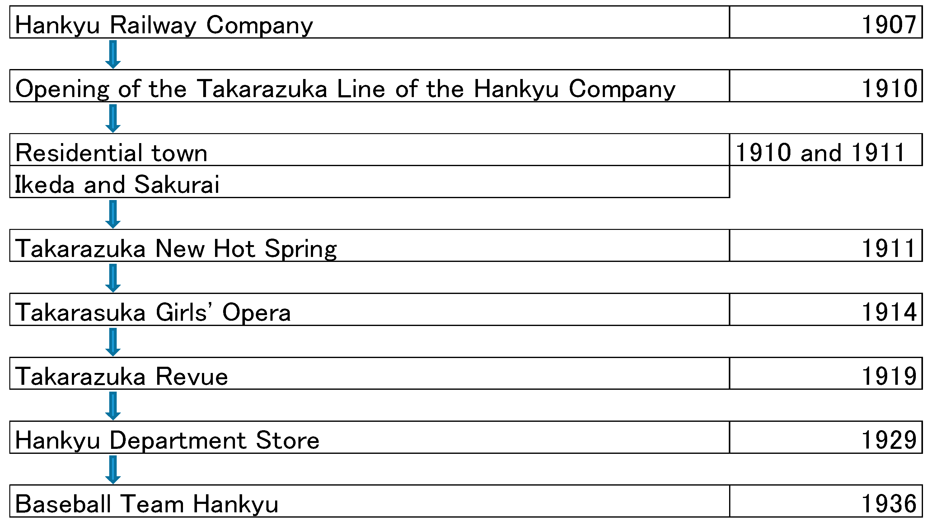
4.1. Hankyu Railway Company in Western Japan, Kanto

Industrialization in Japan created issues such as air pollution and deteriorating sanitary conditions. In light of this, Kobayashi called for the development of residential areas in the nature-rich suburbs outside the city to encourage people to relocate from the central city of Osaka in western Japan, Kansai, which had become a “smoke capital”. According to Kashima (2018), he offered suburban housing to residents under such circumstances. Matsuda (2003) pointed out that the development of suburban residential areas is essential for private railroad management.

Chairman Kazumi Kobayashi of the Hankyu Railway Company succeeded in developing urban agglomeration through the establishment of Hankyu’s private railroad system. He achieved this by building residential cities in the suburbs, whose residents would use the railroad and thus contribute to its management. In the middle of the railroad, he created cultural activities, such as theaters, schools, and hot springs. Residents along the line then used the railroad as a means of transportation from the center to the suburbs and from the suburbs to the center for their activities.

As shown in Figure 4, Hankyu Corporation was founded in 1907 as a private railroad company. It opened its Takarazuka line in 1910, connecting Umeda in the central city of Osaka with Takarazuka. At the same time, it began residential development: in 1910 it built a residential area in Ikeda–Muromachi along the Takarazuka line. In 1910, Hankyu Corporation sold 270 housing units in Ikeda. It also sold 241 housing units in Sakurai in 1911. The Ikeda–Muromachi residential area built along the Hankyu line was the core project of the development model (Ikeda Municipal Library, 2014).

As for cultural activities along the railroad line, Takarazuka New Hot Springs was established in 1911 to attract customers along the Takarazuka route; in 1914, the Takarazuka Girls’ Opera Troupe performed at Takarazuka New Hot Springs, which later became the Takarazuka Revue; in 1919, the Takarazuka Music Opera School was founded as a private school; in 1929, the Hankyu Department Store was established at Umeda Station, Japan’s first terminal, with a total floor space of 10,000 square meters. A baseball team was established in 1936, and a baseball stadium was built the following year (Kuchiki et al., 2017).

The annual number of passengers carried by Hankyu Railways was approximately 3.6 million in 1910, when the company first opened; 20 years later, in 1930, it increased to 48.7 million—around 13 times as many passengers as it carried in its first year (Doi, 2020).

Figure 5, which summarizes the above, shows a station connecting a starting point, where there is a department store; a midpoint, where housing is located; and an ending point with a resort town. There is also an assortment of residential areas, stadiums, and schools along the line. In this case, a school was established closer to the end of the line than the residences. This reversed the morning and evening commute to work and school and reduced train congestion.

In summary, the construction sequence of urban agglomeration policy entails the construction of a railroad, the development of residential areas, and the creation of culture, as shown in Figure 5 (Kuchiki et al., 2017). The construction of a railroad acts as a master switch in urban agglomeration policy, while cultural activities in the service sector are an accelerator. Another case is illustrated in the next subsection.

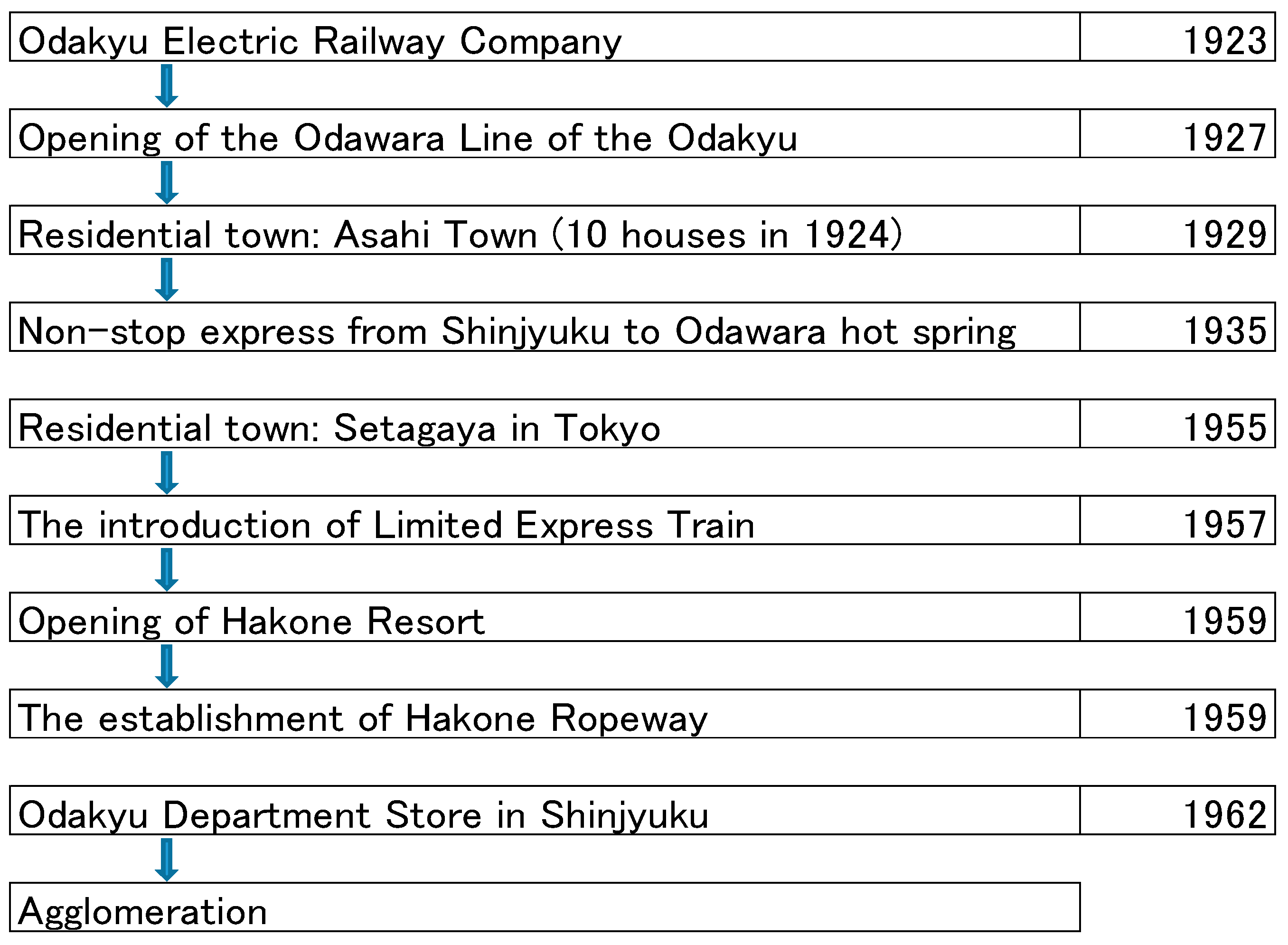
4.2. Odakyu Electric Railway Company in Eastern Japan, Kanto

There are two main economic regions in Japan: Kansai in the west and Kanto in the east. The Hankyu Railroad model in Kansai is a prototype model for developing regions in Japan. The establishment of the Odakyu Railroad in Kanto originated from the Kobayashi model. The line linked Shinjuku in the center of Kanto and Odawara in the suburbs of Kanto. Later, a bullet train linked Odawara in Kanto and Osaka in Kansai. Residential towns, cultural facilities such as museums to enhance the level of culture, and shopping malls were constructed along the Odakyu Line. Agriculture in suburban areas also helped to narrow the gap between the center and the suburbs. We explain the case of Odakyu as shown in Figure 6 (Kuchiki et al., 2017).

In 1923, Nararoku Ando founded the Odakyu Corporation. The Odakyu Line led his company to introduce express trains connecting two cities: Shinjuku in Tokyo and Odawara in Kanagawa Prefecture. Figure 6 charts the flow of the Odakyu Line from the formation of schools in 1925 and 1926, the Odakyu Line in 1927, a residential area in 1929, and a movie theater district and broadcasting station in 1932.

The construction of the residential areas shown in

Table 6. Number of users of Odakyu Electric Railway (unit: person, %).

	1929	1930	1931	1932	1933	1934	1935	1936	Annual Growth Rate
Soshigayaohkura	127,891	269,697	262,949	277,395	287,696	369,794	382,038	428,550	18.8
Seijyogakuen	293,413	661,705	600,200	698,814	714,946	681,274	716,197	754,806	14.4
Kitami	46,948	138,449	85,659	72,098	69,599	71,458	77,583	89,260	9.6
Shimokitazawa	417,052	919,068	1,013,315	1,073,424	1,049,095	837,628	919,614	1,002,019	13.3
Keido	232,470	516,942	577,500	615,558	674,186	717,929	877,786	993,010	23.0
Total	1,117,774	2,505,861	2,539,623	2,737,289	2,795,522	2,678,083	2,973,218	3,267,645	16.5

Source: Calculated by the author based on research by Kuchiki (2015).

increased the total number of passengers at the five Odakyu Line stations from 1,117,774 in 1929 to 3,267,645 in 1936 (Table 5, Kuchiki (2015)). The annual growth rate of 16.5% from 1930 to 1936 proves that the construction of residential areas was effective in the management of the railroad company. The case of the Odakyu Electric Railway helps illustrate that the construction of residential areas is an effective management strategy for railroad companies (Odakyu Electric Railway Co., 2025). In summary, the construction of railroads is a master switch in urban agglomeration policy, while cultural activities in the service sector are an accelerator.

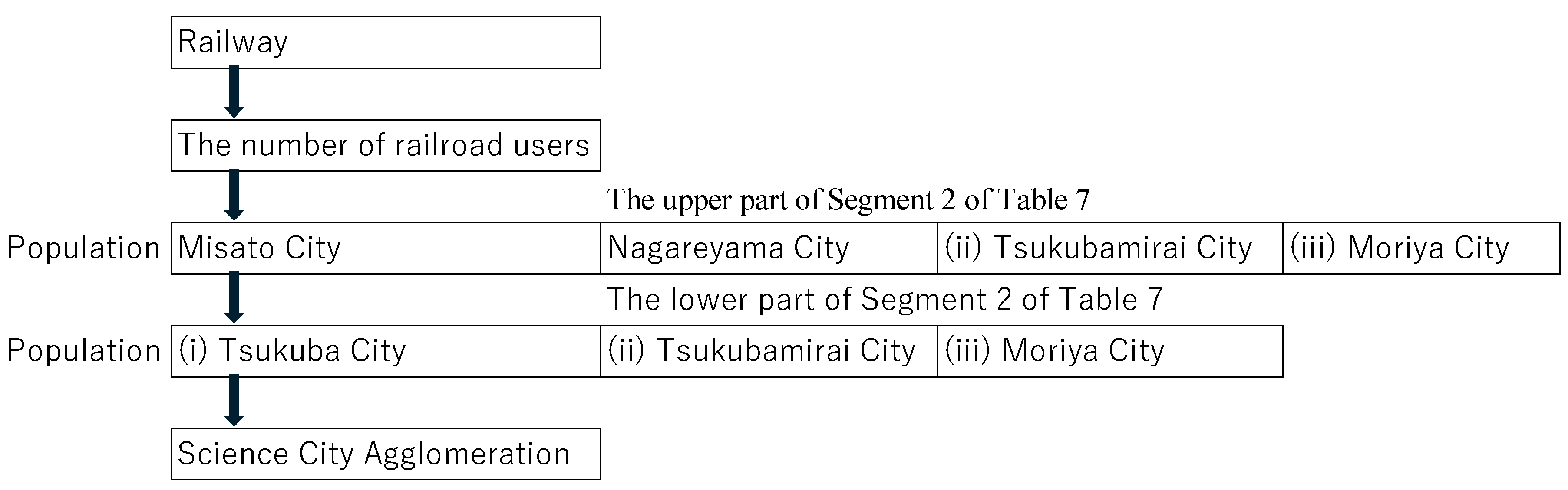
5. The Success of Tsukuba Science City

The Ministry of Land, Infrastructure, Transport and Tourism of Japan coordinated the formation of the urban agglomeration policy shown in Figure 7, based on the decision of the Academic New Town Construction Promotion Headquarters and the “Tsukuba Science City Construction Law”. The Tsukuba Science City agglomeration illustrates the construction sequence.

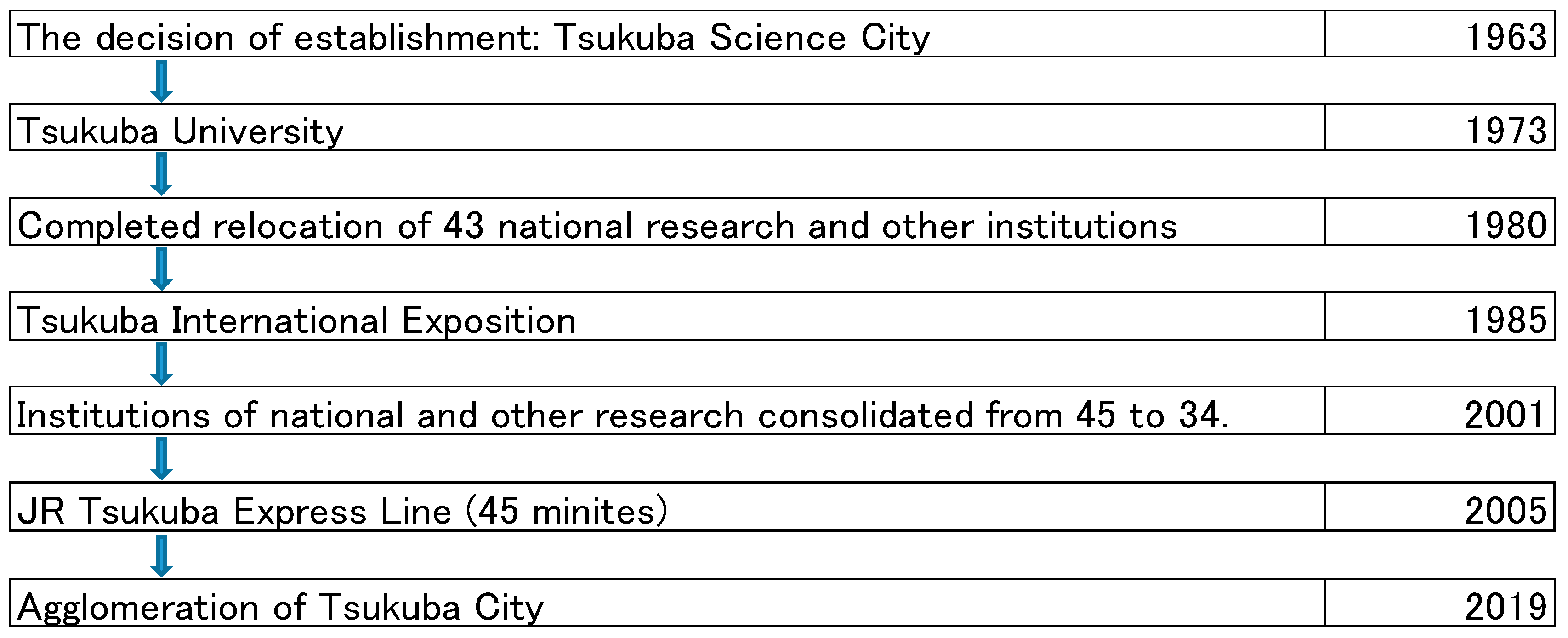
5.1. Tsukuba Science City

Tsukuba Science City was constructed as a national project to mitigate congestion in Tokyo via the planned relocation of national testing and research institutes located in Tokyo and other areas, and to shape a center for advanced research and education. The decision to build Tsukuba Science City was made in September 1963, and the project began in 1968 (City of Tsukuba, 2023; Ministry of Land, Infrastructure, Transport and Tourism of Japan, 2024).

Tsukuba Science City is located in the southern part of Ibaraki Prefecture, approximately 60 km northeast of central Tokyo and 40 km northwest of New Tokyo International Airport. It covers an area of approximately 28,372 hectares (approximately half the size of Tokyo’s 23 wards). The central 2700 hectares of the new town have been developed as a “research and education district”, where national testing and research institutes, educational institutions, commercial and business facilities, and residences are systematically located in a planned development.

The University of Tsukuba was founded in 1975, and the Tsukuba Expo was held in 1985. The relocation and construction of facilities for 43 national testing and research institutes and national universities were almost completed by March 1980. The areas outside of the research and educational districts are called “suburban areas” and are being expanded for the balanced development of the city.

5.2. Tsukuba Express

On 24 August 2005, the Tsukuba Express Line opened for business. The Tsukuba Express connects the Tokyo metropolitan area with Saitama, Chiba, and Ibaraki Prefectures. The fact that the opening of the Tsukuba Express preceded the growth of both residential areas and academic and research campuses is a lesson in determining the construction sequencing of agglomerations.

Tsukuba Science City and its vicinity are the three cities of Tsukuba, Tsukubamirai, and Moriya in Ibaraki Prefecture, the terminus for the Tsukuba Express train. These three cities have six stations: Tsukuba, Research Science Park, Expo Commemorative Park, Midori, Miraidaira, and Moriya, and residential areas were developed in Nakane and Kanetadai in Tsukuba City, Katsuragi in Research Science Park, Expo Commemorative Park, Midori, Miraidaira, and Moriya City. Shopping malls were built at these stations as living areas for the industrial agglomeration centering on the railroad.

5.3. The Railroad as a Master Switch for Science City Agglomeration

Kuchiki (2024b) explains Granger causality as follows: Consider the two variables x and y. Analyses in a time series assume stationary stochastic processes, while drift is an intercept component. It is generally accepted that equations without a drift term are used for stationary stochastic processes. Model 1 is an autoregressive model of y, and Model 2 is an autoregressive model of x and y. Granger causality holds if the prediction error of Model 2 is smaller than that of Model 1. Suppose that the lags of x and y are n (n = 1, 2, 3, 4, or 5, in our models), and e_i (i = 1, 2) is an error term.

Model 1: y(t) = b₁₁y(t − 1) + … + b_1ny(t − n) + e₁,

Model 2: y(t) = b₂₁y(t − 1) + … + b_2ny(t − n) + c₂₁x(t − 1) + … + c_2nx(t − n) + e₂.

In the case where all values of c_2i are 0, x does not Granger-cause y. We applied the F-test to find the causal relationship between research expenses per researcher and value added.

This subsection examines whether the opening of the Tsukuba Express is a master switch in the urban agglomeration policy of Tsukuba Science City and its vicinity of “(i) Tsukuba City, (ii) Tsukubamirai City, and (iii) Moriya City”. The opening of the Tsukuba Express train line caused the agglomeration of the endpoints of the line, i.e., Tsukuba Science City and its vicinity. For these three cities, the increase in the number of rail users Granger-caused population growth in each city.

As shown in the upper part of Segment 2 of

Table 7. Granger causality on railroad users and population.

	Segment 1	Segment 2	p-Value	F-Value	Lag	Time
Saitama Prefecture					Years	Minutes
Misato City	1. the number of “railroad users”	the number of population of Misato City	0.0267 *	5.5729	1	20
	2. the number of population of Misato City	the number of “railroad users”	1.31 × 10−6 ***	40.852	1
	3. the number of population of (i) Tsukuba City	the number of population of Misato City	0.002257 **	8.8762	3
Yashio City	4. the number of population of Yashio City	the number of “railroad users”	6.33 × 10−6 ***	33.057	1	17
Chiba Prefecture
Nagareyama City	5. the number of “railroad users”	the number of population of Nagareyama City	0.0001999 ***	38.843	4	25
	6. the number of population of Nagareyama City	the number of “railroad users”	1.75 × 10−7 ***	52.478	1
Kashiwa City	7. the number of population of Kashiwa City	the number of “railroad users”	3.24 × 10−6 ***	36.25	1	36
Ibaraki Prefecture
Tsukubamirai City	8. the number of “railroad users”	the number of population of (ii) Tsukubamirai City	0.001807 **	9.1563	2	40
	9. the number of population of Tsukubamirai City	the number of “railroad users”	6.47 × 10−8 ***	58.96	1
Moriya City	10. the number of “railroad users”	the number of population of (iii) Moriya City	0.02679 *	4.4557	2	32
	11. the number of population of Moriya City	the number of “railroad users”	6.55 × 10−6 ***	32.899	2
(i) Tsukuba City	12. the number of population of Tsukuba City	the number of “railroad users”	4.13 × 10−7 ***	47.265	1	45
	Agglomeration of population of (i) Tsukuba City, (ii) Tsukubamira City and (iii) Moriya City
	Segment 1	Segment 2 (Agglomeration of Tsukuba Science City)	p-value	F-value	Lag	From Tokyo
Ibaraki Prefecture					Years	Minutes
(i) Tsukubamirai City	13. the number of population of Tsukuba City (i)	the number of population of (ii) Tsukubamirai City	0.01584 *	5.2647	2	40
(ii) Moriya City	14. the number of population of Tsukuba City (i)	the number of population of (iii) Moriya City	0.0589	3.3259	2	32
Chiba Prefecture
Nagareyama City	15. the number of population of Nagareyama	the number of population of (i) Tsukuba City	0.003031 **	8.2388	3	25
Kashiwa City	16. the number of population of Kashiwa	the number of population of (i) Tsukuba City	0.02323 *	6.4298	4	36
Saitama Prefecture
Yashio City	17. the number of population of Yashio	the number of population of (i) Tsukuba City	0.007985 **	10.012	4	17
Misato City	18. the number of population of Misato City	the number of population of (i) Tsukuba City	0.01004 **	9.134	4	20

Note: * significant at 5%, ** significant at 1%, and *** significant at 0%. Source: Calculated by the author based on the data in Appendix B (Table A1).

, the increase in the number of railroad users of the Tsukuba Express Granger-causes population growth in four cities, including Misato City in Saitama Prefecture and Nagareyama City in Chiba Prefecture, which are located between the start and end points of the central cities, and (ii) Tsukubamirai City and (iii) Moriya City in Ibaraki Prefecture, which are located at the end points. Additionally, the population growth of the above four cities Granger-causes population growth in Tsukuba Science City and its vicinity, i.e., (i) Tsukuba City and (ii) Tsukubamirai City, as shown in the lower part of Segment 2 in Table 7. In other words, scientific urban agglomeration is completed.

Varying the number of lags from 1 to 4 serves as a robustness check to examine whether the detected Granger causal relationships are sensitive to the lag structure, as shown in

Table 8. Robustness checks of Granger causality findings.

#	Direction (X → Y)	Lags	With Granger Causality (p < 0.05) Interpretation
1	ex.va → ex.mm	lags 1–3	Moderate causality at short lags
2	ex.mm → ex.va	lag 1 only	Very strong short-term causality
3	ex.pt → ex.mm	lags 1–3	Strong consistent causality
4	ex.py → ex.va	lags 1–2	Strong short-term causality
5	ex.va → ex.pn	lags 3–4	Causality appears only at higher lags
6	ex.pn → ex.va	lags 1, 3	Strong but irregular pattern
7	ex.pk → ex.va	lag 1 only	Strong short-term effect
8	ex.va → ex.pf	lags 2, 4	Evidence of delayed causality
9	ex.pf → ex.va	lags 1, 3	Strong at lag 1, weaker later
10	ex.va → ex.pm	lag 2 only	Weak evidence
11	ex.pm → ex.va	lag 1 only	Strong short-term causality
12	ex.pt → ex.va	lags 1, 3	Strong short-term, possible mid-term effect
13	ex.pt → ex.pf	lag 2 only	Weak evidence
14	ex.pt → ex.pm	No lags < 0.05	No causality
15	ex.pn → ex.pt	lags 2–4	Strong delayed causality
16	ex.pk → ex.pt	lag 4 only	Weak and delayed effect
17	ex.py → ex.pt	lag 4 only	Delayed causality only
18	ex.mm → ex.pt	lag 4 only	Only very delayed causality

Source: Compiled by the author.

. If the causality remains significant across multiple lag lengths, the results can be considered more robust and less dependent on a specific lag specification.

If the causality remains significant across multiple lag lengths, the results can be considered more robust and less dependent on a particular lag specification. Tsukuba City was founded in 1987, and the Tsukuba Express train began to operate in 2005. The population growth rate during this period was 0.95%. However, after the operation started, the population in 2015 was 226,963, and the population growth rate from January 2005 to January 2015 was 1.24%—a significant increase (Ibaraki Preferential Government, 2025).

The start of the Tsukuba Express service resulted in an average annualized difference of 0.3% between the 10 years before and the 10 years after it began operating. Tsukuba City ranked first in Japan for the first time with a population growth rate of 2.30% as of 2023 and continued to rank first in 2024. These changes were primarily attributed to the inflow of tourists and the Tsukuba Express (City of Tsukuba, 2023).

In summary, the construction sequencing resulted in the following sequence: the opening of a railroad as a master switch, the development of residential towns, and the activity of education and research in the service sector as an accelerator, as shown in Figure 8.

6. Conclusions

This paper presents the concept of “sequencing economics” with respect to the segments of agglomeration, consisting of (A) segmentation, (B) construction sequencing, and (C) function. This paper established the following two hypotheses for agglomeration policy, as shown in

Table 9. Railroad-driven agglomeration (RDA).

(i) Spatial economics: Fujita and Krugman	(i) Master switch	(i) Lower transport costs
(ii) Input output table: Forward linkage effect	(ii) Accelerator	(ii) Service sector
Function in Sequencing economics	(i) Master switch	(i) Railroad
	(ii) Accelerator	(ii) Cultural activities
Transit-Oriented Development (TOD)	Cases: Hankyu Railway of Japan	Railroad-Driven Agglomeration (RDA)
Agglomeration (RDA)	(i) Master switch	(i) Tsukuba Express
Finding: Tsukuba Science City	(ii) Accelerator	(ii) Research and education

Source: Compiled by the author.

. First, a master switch is the construction of a segment that lowers “transport costs”, derived from the monocentric city model of spatial economics by Fujita and Krugman (1995). Second, accelerators are activities in “the service sector” that have the highest forward-linkage effect in the input–output relationship. Regarding science city agglomeration policy, it can be concluded that high-speed rail is the master switch, and research and education activities are the accelerator.

In this paper, we analyzed a case of science city agglomeration that emerges from a monocentric city as railway-driven agglomeration (RDA)—a type of transit-oriented development (TOD)—in order to focus on the effective construction of the segments of the agglomeration. The Hankyu Corporation and Odakyu Corporation are examples in Japan. This paper demonstrates that the Tsukuba Express, as a case study of RDA, Granger-caused the agglomeration of Tsukuba Science City. By using an express railroad as a master switch and the activity of research and education as an accelerator, a second science city can emerge from the monocentric city.

The policy implications are as follows. We have identified railroads as the “master switch” that allows countries to escape the middle-income trap, which can be applied to various companies of this economic status. The median income of middle-income countries has never been more than one-tenth of that of the United States in the past 50 years. By turning on “the master switch”, the activation of agglomeration policies can be ensured, enabling middle-income countries to improve their financial status.

Some examples are the railroads between Singapore and Iskandar in Johor, Malaysia, and between Ho Chi Minh City and Dalat City in Lam Dong Province, Vietnam. High-speed railroads will be constructed as a master switch for agglomeration construction. The next step is to “accelerate” the activities of research and education, for the purpose of economic development.

This paper establishes sequencing economics, a policy implementation rule that is based on sequential equations, as opposed to Tinbergen’s rule, which is based on simultaneous equations.

However, several issues remain. Firstly, it is necessary to identify master switches for other new cities that are focusing on constructing railroads and increasing the availability of cultural activities by taking up a number of other cases. Secondly, the critical path method (CPM) and building information modeling (BIM) of the scientific management method should be explicitly incorporated into sequencing economics to achieve a more efficient implementation of agglomeration policy. Thirdly, it is necessary to specify functions in sequencing economics, e.g., by deepening the discussion on whether the sequence is the beginning or the middle of the construction of environmental segments, in order to make transit-oriented development sustainable.

References

1. Alonso, W. (1964). Location and land use. Toward a general theory of land Rent. Harward University Press. [Google Scholar] [CrossRef]
2. Audretsch, D. B., & Feldman, M. P. (1996). R&D spillovers and the geography of innovation and production. American Economic Review, 86(3), 630–640. [Google Scholar]
3. Calthorpe Associates. (1992). City of San Diego land guidance system: Transit-oriented development design guidelines. City of San Diego & Calthorpe Associates. [Google Scholar]
4. Calthorpe, P. (1993). The next American metropolis: Ecology, community, and the American dream. Princeton Architectural Press. [Google Scholar]
5. City of Tsukuba. (2023). What is Tsukuba science city? Available online: https://www.city.tsukuba.lg.jp/soshikikarasagasu/toshikeikakubutoshikeikakuka/gyomuannai/4/3/1002135.html (accessed on 4 December 2024).
6. City of Tsukuba. (2024). Available online: https://www.city.tsukuba.lg.jp/shisei/joho/jinkohyo/index.html (accessed on 6 December 2024).
7. Doi, T. (2020). TOD in 1910—Establishment and development of the urban railroad business model in Kansai. In City planning review (Vol. 346, pp. 30–33). The City Planning Institute of Japan. Available online: https://chikoken.org/wp/wp-content/uploads/toshi030-033.pdf (accessed on 7 December 2024).
8. Fogelson, R. M. (1967). The fragmented metropolis: Los Angeles, 1850–1930. University of California University Press. [Google Scholar]
9. Fujita, M., & Krugman, P. (1995). When is the economy monocentric?: Von Thünen and Chamberlin unified. Regional Science and Urban Economics, 25, 505–528. [Google Scholar] [CrossRef]
10. Fujita, M., & Thisse, J.-F. (2003). Does geographical agglomeration foster economic growth? And who gains and loses from it? Japanese Economic Review, 54, 121–45. [Google Scholar] [CrossRef]
11. Gantt, H. L. (1910). Work, wages and profits: Their influence on the cost of living. Engineering Magazine Company. [Google Scholar]
12. Golizadeh, H. (2017). Automated construction progress monitoring using image segmentation methods and BIM. LAP Lambert Academic Publishing. [Google Scholar]
13. Helpman, E., & Krugman, P. (1985). Market structure and foreign trade. The MIT Press. [Google Scholar]
14. Hilton, G. W., & Due, J. F. (1960). The electric interurban railways in America. Stanford University Press. [Google Scholar]
15. Howard, E. (1902). Garden cities of tomorrow. Swan Sonnenschein & Co., Ltd. Available online: https://dn790002.ca.archive.org/0/items/gardencitiesofto00howa/gardencitiesofto00howa.pdf (accessed on 9 March 2025).
16. Ibaraki Preferential Government. (2025). Population. Available online: https://www.pref.ibaraki.jp/kikaku/tokei/fukyu/tokei/sugata/local/tsukuba.html?utm_source=chatgpt.com (accessed on 9 March 2025).
17. Ikeda Municipal Library. (2014). Muromachi housing. Ikeda City Library. Available online: https://lib-ikedacity.jp/kyodo/kyodo_bunken/muromachi_jutaku.html (accessed on 10 July 2025).
18. Institute of Developing Economies-JETRO. (2006). Asian international input-output table 2000: Volume 2 data, statistical data series (p. 315). No. 90. Institute of Developing Economies-JETRO. [Google Scholar]
19. Jamme, H.-T., Rodriguez, J., Bahl, D., & Banerjee, T. (2019). A twenty-five-year biography of the TOD concept: From design to policy, planning, and implementation. Journal of Planning Education and Research, 39(4), 409–428. [Google Scholar] [CrossRef]
20. JICA. (2014). Information collection and confirmation study on ASEAN 2025: Final report. Available online: https://openjicareport.jica.go.jp/pdf/12152906.pdf (accessed on 7 December 2024).
21. Johnston, R. B., & Sundararajan, V. (Eds.). (1999). Sequencing financial sector reforms: Country experiences and issues. International Monetary Fund. [Google Scholar] [CrossRef]
22. Kashima, S. (2018). The great management innovator born in Japan, Ichizo Kobayashi. Chuokoron Shinsha Company. [Google Scholar]
23. Kashiwa City. (2024). Available online: https://www.city.kashiwa.lg.jp/databunseki/shiseijoho/toukei/jinko/joju.html (accessed on 6 December 2024).
24. Kelley, J. E., Jr., & Walker, M. R. (1959). Critical path planning and scheduling proceedings of the eastern joint computer conference. Available online: https://mosaicprojects.com.au/PDF/PM-History_Critical_Path_Planning_&_Scheduling_Kelley_and_Walker_1959.pdf (accessed on 4 January 2025).
25. Krugman, P. (1991). Increasing returns and economic geography. Journal of Political Economy, 99, 483–99. [Google Scholar] [CrossRef]
26. Kuchiki, A. (2015). Building a “sixth industrial cluster in the form of a cobweb type of train-led cluster” as a growth strategy for Asia. International Trade and Investment, (101). Available online: https://www.iti.or.jp/kikan101/101kuchiki.pdf (accessed on 10 January 2025). (In Japanese).
27. Kuchiki, A. (2023). Accelerator for agglomeration in sequencing economics: “Leased” industrial zones. Economies, 11, 295. [Google Scholar] [CrossRef]
28. Kuchiki, A. (2024a). Brake segment for agglomeration policy: Engineers as human capital. Economies, 12, 163. [Google Scholar] [CrossRef]
29. Kuchiki, A. (2024b). Start switch for innovation in “construction sequencing”: Research funding. Economies, 12, 302. [Google Scholar] [CrossRef]
30. Kuchiki, A., Gokan, T., & Maruya, T. (2017). Railway-led formation of the agriculture-food-tourism industry cluster. In A. Kuchiki, T. Mizobe, & T. Gokan (Eds.), A multi-industrial linkages approach to Cluster (pp. 187–205). Chapter 9. Palgrave Macmillan. [Google Scholar]
31. Kuchiki, A., & Sakai, H. (2023). Symmetry breaking as “master switch” for agglomeration policy. Review of Public Administration and Management, 11(2), 1–8. [Google Scholar] [CrossRef]
32. Kuchiki, A., & Tsuji, M. (Eds.). (2008). The flowchart approach to industrial cluster policy. Palgrave Macmillan. [Google Scholar]
33. Malcolm, D. G., Roseboom, J. H., Clark, C. E., & Fazar, W. (1959). Application of a technique for research and development program evaluation. Operations Research, 7(5), 646–669. Available online: https://econpapers.repec.org/article/inmoropre/v_3a7_3ay_3a1959_3ai_3a5_3ap_3a646-669.htm (accessed on 4 January 2025). [CrossRef]
34. Matsuda, A. (2003). The development of residential towns in the suburbs and strategies of private railroad companies. Japanese Journal of Human Geography, 55(5), 492–508. [Google Scholar] [CrossRef]
35. Ministry of Economy, Trade and Industry of Japan. (2024). Monthly report of indices of tertiary industry activity. Available online: https://www.meti.go.jp/english/statistics/tyo/sanzi/result-2.html#historical (accessed on 2 December 2024).
36. Ministry of Land, Infrastructure, Transport and Tourism of Japan. (2024). Available online: https://www.mlit.go.jp/common/001447956.pdf (accessed on 4 December 2024).
37. Misato City. (2024). Available online: https://www.city.misato.lg.jp/soshiki/somu/somu/3/2/1310.html (accessed on 6 December 2024).
38. Moriya City. (2024). Available online: https://www.city.moriya.ibaraki.jp/_res/projects/default_project/_page_/001/005/527/201901joju.pdf (accessed on 6 December 2024).
39. Nagareyama City. (2024). Available online: https://www.city.nagareyama.chiba.jp/appeal/1003878/1003882.html (accessed on 6 December 2024).
40. National Diet Library of Japan. (2025). Takarazuka hot spring. National Diet Library of Japan. Available online: https://www.ndl.go.jp/scenery/column/kansai/takarazuka_onsen.html (accessed on 9 March 2025).
41. Odakyu Electric Railway Co. (2025). Available online: https://www.odakyu.jp/company/history/ (accessed on 10 July 2025).
42. Porter, M. E. (1998). Clusters and the new economics of competition. Harvard Business Review, 76(6), 77–90. [Google Scholar] [PubMed]
43. Rodrik, D. (2007). One economics, many recipes: Globalization, institutions, and economic growth. Princeton University Press. [Google Scholar]
44. Taylor, F. W. (1911). The principles of scientific management. Harper Brothers. Available online: https://resources.saylor.org/wwwresources/archived/site/wp-content/uploads/2011/08/HIST363-7.1.3-Frederick-W-Taylor.pdf (accessed on 1 January 2025).
45. Tinbergen, J. (1952). On the theory of economic policy. North-Holland. [Google Scholar]
46. Tsuganezawa, S. (1991). Takarazuka strategy. Kodansha. [Google Scholar]
47. Tsukubamirai City. (2024). Available online: https://www.city.tsukubamirai.lg.jp/gyousei/shoukai/page000783.html (accessed on 6 December 2024).
48. Warner, S. B. (1962). The process of growth in Boston, 1870–1900. Harvard University Press. [Google Scholar]
49. World Bank. (2024). World development report 2024: The middle-income trap. World Bank. Available online: https://www.worldbank.org/en/publication/wdr2024 (accessed on 9 March 2025).
50. Yashio City. (2024). Available online: https://www.city.yashio.lg.jp/shisei/tokei/toukeiyashio/R5toukeiyashio.files/yashio_r5toukeisho.pdf (accessed on 10 July 2025).
51. Zalduendo, J. (2005). Pace and sequencing of economic policies. IMF working paper. WP/05/118. Available online: https://www.imf.org/external/pubs/ft/wp/2005/wp05118.pdf (accessed on 9 March 2025).
Figure 1. The monocentric spatial configuration. Source: Fujita and Krugman (1995).
Economies 13 00204 g001
Figure 2. The input–output relationship of a farm. Source: Compiled by the author.
Economies 13 00204 g002
Figure 3. Sequence in the formation of railroad-driven agglomeration. Source: Compiled by the author.
Economies 13 00204 g003
Figure 4. Hankyu model. Source: Compiled by the author based on research by Tsuganezawa (1991), National Diet Library of Japan (2025), and Kuchiki et al. (2017).
Economies 13 00204 g004
Figure 5. Two-pole cities. Source: Compiled by the author.
Economies 13 00204 g005
Figure 6. Odakyu Corporation in Japan. Source: Compiled by the author.
Economies 13 00204 g006
Figure 7. Agglomeration of Tsukuba Science City. Source: Compiled by the author.
Economies 13 00204 g007
Figure 8. Science city agglomeration. Source: Compiled by the author.
Economies 13 00204 g008