Steadying the Ship: Can Export Proceeds Repatriation Policy Stabilize Indonesian Exchange Rates Amid Short-Term Capital Flow Fluctuations?

Abstract

This paper investigates the impact of repatriated export proceeds on exchange rate volatility in Indonesia. By applying a time-varying parameter vector autoregression (TVP-VAR) model with stochastic volatility, we assess whether the impact of repatriated export proceeds can dampen the effect of short-term capital flows. Our findings indicate that the influence of export proceeds on exchange rate volatility varies over time, with no evidence supporting its ability to dampen the impact of short-term capital flows in the short and intermediate terms. Furthermore, we identify a reversal pattern in the impacts of both repatriated export proceeds and short-term foreign capital flows after 3–5 days, suggesting a potential need to evaluate policies aimed at dampening short-term capital flow impacts on exchange rate volatility. Our results are robust across a range of sensitivity and robustness checks, confirming the reliability of our findings.

1. Introduction

In order to stabilize their currencies, several developing economies with non-pegged exchange rate regimes have regulated how corporations receive export proceeds. Broadly speaking, those economies require export proceeds to be repatriated1 through domestic foreign exchange banks within a specified period.

In Indonesia’s case, the regulation was initially meant to lessen the dependence on short-term foreign capital flows, improve the continuity of the domestic foreign exchange supply, and stabilize the Indonesian rupiah (IDR). When it was first introduced in September 2011, the USD/IDR exchange rate was heavily depreciated. Moreover, the foreign portfolio in stocks, government bonds, and central bank bills was USD 5.5 billion, which was only 17% of the average volume of residents’ export proceeds placed abroad.

Considering the massive volume of export proceeds kept abroad compared to the foreign short-term portfolio, it is evident that voluntary repatriation is not the norm for most export proceeds in Indonesia. It influences the foreign exchange supply in the Indonesian foreign exchange market and, in turn, may affect exchange rates (Dominguez & Frankel, 1993). Furthermore, the shallow exchange market attracts short-term capital inflows (Reinhart & Reinhart, 2009).

In the beginning, the policy required exporters to repatriate the payments they received from the exports, i.e., the export proceeds, 90 calendar days after the export took place which in 2014 revised to the end of the third month after the exports took place. Several revisions after 2014 basically revised the procedures for reporting the export proceeds received.

Nevertheless, both before and after the revisions of the policy, there is neither a requirement for exporters nor recipients of export proceeds to convert the export proceeds into the local currency (Indonesian rupiah), nor is there a minimum period during which the fund should be kept in the Indonesian financial system. These features that seem to weaken the effect of the regulations were due to the free capital movement policy adopted by Indonesia. The policy requires Indonesia to follow the 2012 International Monetary Fund (IMF) Institutional View (IV) on Capital Flow Management.

This paper scrutinizes the impact of Indonesia’s export proceeds repatriation policy on exchange rate volatility. Specifically, we analyze whether the volume of repatriated export proceeds acts as a buffer for short-term foreign capital flows and how its influence compares to the impact of short-term foreign capital flows on exchange rate volatility. Despite the widespread application of similar policies across various countries, the effectiveness of export proceeds repatriation policy in stabilizing exchange rate volatility has, to the best of our knowledge, never been thoroughly analyzed, making this study a pioneering effort on the topic. Consequently, this paper represents the first policy evaluation focused on export proceeds repatriation policy, with Indonesia serving as the case study.

Indonesia presents an ideal case for this analysis, as it is one of the world’s top exporters of key commodities such as palm oil, coal, and rubber, and has implemented the export proceeds repatriation policy for more than a decade, providing ample data for analyzing its effect on the economy. Moreover, throughout the policy’s implementation, Indonesia has adhered predominantly to a floating exchange rate regime, as classified by the IMF. This provides a suitable environment for examining the interaction between export proceeds, short-term capital flows, and exchange rate volatility.

The remainder of this paper is structured as follows. Section 2 summarizes the key literature on export proceeds. Section 3 introduces the data and describes our empirical strategy. Section 4 presents the results and empirical analysis. Section 5 discusses the robustness tests. Finally, Section 6 concludes this paper.

2. Literature Review

Worldwide, in 2021, 832 emerging countries adopted the policy of export proceeds repatriation. However, given the common adoption of the policy among non-pegged exchange rates in developing countries, the literature on export proceeds is very limited. Earlier studies were more concerned with stabilizing export proceeds amidst fluctuations in commodity prices and export quantities. For example, Wallich (1961) scrutinized the export proceeds stabilization from raw materials; Powell (1959) questioned the effectiveness of increasing supply to expand the volume of export proceeds in the wool industry; Massell (1964) highlighted that policies aimed at diversifying sources of export proceeds do not necessarily stabilize export proceeds; while Macbean (1962) took a broader view on the importance of quantity fluctuations of exports on the stability of export proceeds in underdeveloped countries. Later studies took different views of export proceeds, seeing export proceeds more as a part of trade balance (Guillaumont, 1980) or, more recently, as a factor that influences foreign direct investment (Asiedu & Lien, 2004; Prayoga & Purnomo, 2024). Hence, this paper will also be one of the very scarce studies on export proceeds, particularly on the impact of export proceeds repatriation on exchange rate volatility.

In light of the literature, the focus of research on exchange rates in developing economies centers primarily on two key aspects: the impact of exchange rates on economic outcomes, particularly growth, and the influence of institutional factors such as trade and financial openness, as well as exchange rate regimes, on exchange rate fluctuations. This body of literature consistently emphasizes the negative effects of exchange rate volatility on long-term economic performance (Aghion et al., 2009; Aysun, 2024; Baum & Caglayan, 2010; Bush & López Noria, 2021; Choudhri & Hakura, 2006; Devereux & Engel, 2002; Feldmann, 2011; Grier & Grier, 2006; Krol, 2014; Lee-Lee & Hui-Boon, 2007). This paper, on the other hand, takes a rather opposite direction and examines the impact of repatriated export proceeds and short-term capital flows on exchange rate volatility. Several studies in this area highlight that different factors affect exchange rate volatility in developing countries compared with the rest of the world (Grossmann & Orlov, 2014). Flood and Rose (1999) show that macroeconomic factors are not essential while Rafi and Ramachandran (2018), Caporale et al. (2017), and Gabaix and Maggiori (2015) highlight the importance of foreign capital flows.

The interrelationships between variables affecting exchange rate volatility change over time, especially when there are structural changes, thus imply that the VAR coefficients should also vary over time. To accommodate the time-varying features, we use a Bayesian econometric approach, the time-varying parameter vector autoregression (TVP-VAR) model with stochastic volatilities, following Primiceri (2005) and Negro and Primiceri (2015). This model is one of the most popular methods for analyzing the interrelationships between variables that change over time. The use of this model in the study of the determinants of exchange rate volatility in Indonesia has also not been exploited much.

3. Data and Empirical Methodology

3.1. Data

To examine the impact of repatriated export proceeds and short-term capital flows on exchange rate volatility, this paper utilizes the TVP-VAR model with five variables as discussed in Section 3.2. The datasets are daily, following the working days of the central bank of Indonesia, Bank Indonesia, from 1 January 2012 to 31 December 2021. Hence, the period of data covers the period from the beginning of the enforcement of the export proceeds repatriation policy in Indonesia until the COVID-19 pandemic. The period also coincides with the stable exchange rate period and the economic crisis following the COVID-19 pandemic. Therefore, this study covers significant regulatory changes, stable economic periods, and major global shocks, providing a comprehensive view of where various factors influence exchange rate volatility.

The vector of the endogenous variables that the TVP-VAR model aims to explain can be expressed as follows:

$$\begin{array}{c}\hfill {\mathbf{y}}_t=\left[\begin{array}{c}IR{D}_t\\ T{V}_t\\ STC{F}_t\\ E{P}_t\\ ER{V}_t\end{array}\right]\end{array}$$

(1)

where $IR{D}_t$ is interest rate differentials between USD and IDR overnight deposit rates from Refinitiv Eikon on day t, dismissing the days that are not the working days of Bank Indonesia. $T{V}_t$ is the net trading volume of foreign exchange transactions on the day t in US dollar, retrieved from Indonesian banks’ daily foreign exchange transaction reports to Bank Indonesia. $STC{F}_t$ is the short-term capital flows on day t in US dollar, consisting of non-resident stock trading flows, non-resident government bond trading flows, and non-resident central bank bills trading flows. The non-resident stock trading flows are retrieved from transaction data from the Indonesian Stock Exchange (IDX); the non-resident government bonds trading flows are retrieved from transaction settlement data from the Ministry of Finance of Indonesia; while the non-resident central bank bills trading flows are retrieved from transaction data from Bank Indonesia.

$E{P}_t$ is the inflow of repatriated export proceeds received by exporters on day t, which is reported to Bank Indonesia through Indonesian banks. This research accumulates export proceeds received on non-working days of Bank Indonesia into the next closest working day to align the data with other data used for this research. The export proceeds data came in different currencies and were converted to USD using the daily mid-closing rates from Refinitiv Eikon. $ER{V}_t$ is the exchange rate volatility on day t as estimated by stochastic volatility using the model in Section 3.3. To estimate the volatility, we use the daily bid closing exchange rate from Refinitiv Eikon and, as before, dismiss the days that are not the working days of Bank Indonesia.

When applying Cholesky decomposition, as outlined by Primiceri (2005), the ordering of variables in the TVP-VAR model is crucial. Following guidance from the literature (Enders, 2015), we arrange the variables in decreasing order of exogeneity. The IRD is considered the most exogenous variable relative to the others (Ulm & Hambuckers, 2022), as it is usually influenced by changes in macroeconomic and monetary policies and is not immediately affected by short-term fluctuations in trading and capital flows (Primiceri, 2005; Ulm & Hambuckers, 2022). It is followed by TV, as suggested by Devereux and Engel (2002) and Enders (2015), as it tends to react to changes in fundamentals such as IRD but has a more immediate effect on capital flows and volatility. EP is more responsive to economic conditions such as interest rates and capital flows and can influence ERV (Enders, 2015; Narayan, 2022). Furthermore, our hypothesis posits that STCF exerts a more significant influence on ERV than EP, leading us to position STCF before EP does in the ordering. Finally, in line with Devereux and Engel (2002) and Primiceri (2005), and given our focus on ERV as the primary outcome variable and its hypothesized position as the most endogenous variable, we place ERV last in the ordering sequence.

3.2. TVP-VAR for Exchange Rate Volatility and Repatriated Export Proceeds

Lane (2001) argues that VAR-based models provide useful empirical evidence by generating impulse response functions to gain insight into the validity of the models. Notable contributions to this field include Clarida and Gali (1994) and Eichenbaum and Evans (1995), who employed VAR models to prove that monetary shocks move the exchange rate consistent with the predictions of sticky-price models.

While the VAR method is powerful, the possibility of the existence of structural changes in macroeconomic settings or the financial environment requires a different treatment when performing an empirical study. The interrelationships between variables affecting exchange rate volatility change over time, especially when there are significant changes, thus implying that the VAR coefficients should change over time. To accommodate the time-varying features, we use a TVP-VAR model with stochastic volatilities to study the impact of export proceeds on Indonesian exchange rate volatility, following Primiceri (2005) and Negro and Primiceri (2015).

The model setup will be using three lags; hence, in the following inter alia, Primiceri (2005), and Nakajima (2011), we have the reduced from the VAR model:

$${\mathbf{y}}_t={\mathbf{c}}_t+{\mathbf{B}}_{1,t}{\mathbf{y}}_{t-1}+{\mathbf{B}}_{2,t}{\mathbf{y}}_{t-2}+{\mathbf{B}}_{3,t}{\mathbf{y}}_{t-3}+{\mathbf{A}}_t^{-1}{\Sigma }_t{\mathbf{ϵ}}_t,t=1,\dots ,T$$

(2)

$$\mathtt{Var}\left({ϵ}_t\right)=I_n$$

with ${\mathbf{y}}_t$ defined as in Equation (1).

Here, ${\mathbf{y}}_t$ is a vector of observed endogenous variables with definitions consistent with those in Section 3.1, ${\mathbf{c}}_t$ is a $5\times 1$ vector of time-varying intercepts; ${\mathbf{B}}_{i,t},i=1,\dots ,k$ are $5\times 5$ matrices of time-varying coefficients; ${\mathbf{A}}_t$ is a lower triangular matrix with ones on the main diagonal and time-varying coefficients below it; ${\Sigma }_t$ is a diagonal matrix of time-varying standard deviations; and ${\mathbf{ϵ}}_t$ is a $5\times 1$ vector of unobservable shocks.

The unknowns in the model are volatilities ${\Sigma }^T$, the coefficients $B^T$ and $A^T$, and the covariance matrix V which we derive in Appendix A. We will define $\theta \equiv [B^T,A^T,V]$. Using the method of Kim et al. (1998), we approximate each element of $\log {ϵ}_t^2$ with a mixture of normals with a mixture indicators $s^T\equiv {\left\{s_t\right\}}_{t=1}^T$. The procedure to obtain posterior draws for ${\Sigma }^T,s^T$ and $\theta$ is given in Appendix D. From the algorithm, we will obtain the estimates of $\theta \equiv [B^T,A^T,V]$. In particular, we will have the time-varying coefficient matrices $B_{i,t},i=1,2,3,t=1,\dots ,T$.

The first 200 days (1 January 2012 to 23 October 2012) are used to calibrate the prior distribution. Following Primiceri (2005) and Negro and Primiceri (2015), the 200 training samples and a time-invariant VAR are used to produce an ordinary least square (OLS) estimate of the VAR coefficients as a prior for $B_0$ and $A_0$ and the associated covariance matrix. The data are normalized before being used to calibrate the prior and estimate the time-varying parameters. We base the simulations on 10,000 iterations of the Gibbs sampler and discard the first 2000 iterations for convergence. Furthermore, since the model theoretically depends on the ordering of the variables (Primiceri, 2005), a robustness check using different ordering is also performed in Section 5. All computations are performed via MATLAB R2023b Student Version.

We aim to examine the extent to which the export proceeds repatriation policy significantly affects exchange rate volatility. Additionally, this methodology will test the hypothesis that, under the current repatriation policy, export proceeds do not function effectively as a buffer against short-term foreign capital flows. Specifically, we will investigate whether repatriated export proceeds and short-term capital flows influence exchange rate volatility in a manner that allows them to substitute for each other.

3.3. Stochastic Volatility with Mixture Sampling

The exchange rate volatility is estimated following the stochastic volatility model parameters. Stochastic volatility models can describe data better than a tightly parameterized model such as GARCH models can (Daníelsson, 1998). Furthermore, owing to the independent modeling of the parameters explaining persistence and kurtosis, these models can better represent empirical regularities (Carnero et al., 2004) and also allow greater flexibility by assuming that the variance of returns has a process that is independent of the process of the returns (Alanya & Rodríguez, 2018). In stochastic volatility models, volatilities are dynamic latent variables. Thus, closed forms of the likelihood functions are more difficult to construct, resulting in a non-standard estimation method (see Morimune, 2007). Hafner and Preminger (2010) acknowledged several popular methods for estimating the likelihood functions. Morimune (2007), Daníelsson (1998), and Jacquier et al. (1994) showed that the more efficient methods are Bayesian Markov Chain Monte Carlo (MCMC) and simulated maximum likelihood (SML). In this paper, we will employ the MCMC method.

The stochastic volatility model for regularly spaced data is

$$y_t=\beta e^{{\displaystyle \frac{h_t}{2}}}{ϵ}_t$$

(3)

where $y_t$ is the mean-corrected exchange rate return with $t=1,\dots ,T$ and ${ϵ}_t\sim N(0,1)$.

The conditional variance of $y_t$ given $h_t$ is $Var\left(y_t\right|h_t)=e^{h_t}$, implying that the conditional variance is time-varying. We assume that $h_t$, the log-volatility of the exchange rate return $y_t$ at time t, follows

$$h_{t+1}=\mu +\varphi (h_t-\mu )+{\sigma }_{\eta }{\eta }_t$$

(4)

where $\varphi$ can be thought as the persistence in the volatility, ${\sigma }_{\eta }$ is the volatility of the log-volatility while ${\eta }_t\sim N(0,1)$ and $h_1\sim N\left(\mu ,{\displaystyle \frac{{\sigma }^2}{1-{\varphi }^2}}\right)$. For identifiability reasons, following Kim et al. (1998), $\beta$ will be set to one when we estimate the model. Finally, ${ϵ}_t$ and ${\eta }_t$ are uncorrelated standard normal noise shocks.

Equation (3) can be rewritten as

$$\log y_t^2=\mu +h_t+\log {ϵ}_t^2.$$

(5)

Thus, the estimation of stochastic volatility models requires the estimation of the parameters

$$\theta =\{\mu ,\varphi ,{\sigma }_{\eta }\}.$$

(6)

and we use an auxiliary mixture sampler following Kim et al. (1998) to estimate them.

Since the volatility is a latent variable, we need to compute $h_t|Y_t,\theta$ for each value of $Y_t=(y_1,\dots ,y_t)$ by particle filtering. We will employ the algorithm of particle filtering following Kim et al. (1998) and Pitt and Shephard (1999).

We first introduce a small constant “offset” $c={10}^{-4}$ (see Fuller, 1996) and set $y_t^{*}=\log (y_t^2+c)$ in order to avoid numerical problems when $y_t$ is close to zero. Thus, we can rewrite Equation (5) into

$$y_t^{*}=h_t+{ϵ}_t^{*},$$

(7)

where ${ϵ}_t^{*}=\log {ϵ}_t^2$.

The error term ${ϵ}_t^{*}$ no longer has a normal distribution, and its density can be written in terms of an auxiliary random variable $s_t\in \{1,\dots ,K\}$ that represents the mixture component indicator such that

$$\begin{array}{c}\hfill \left({ϵ}_t^{*}\right|s_t=i)\sim N(m_i-1.2704,v_i^2),\\ \hfill \mathtt{Pr}(s_t=i)=p_i.\end{array}$$

(8)

Kim et al. (1998) proposed that $K=7$ and $\{m_i,p_i,v_i^2\}$ given in Appendix B make the mixture approximation sufficiently good.

Equation (8) representation is the best method to estimate mixture models. In employing MCMC procedures, our stochastic volatility in Equations (4) and (7) is now conditionally linear normal given the component indicators $s=(s_1,\dots ,s_T)$. The posterior density that will be of interest is $\pi (s,h,\varphi ,{\sigma }_{\eta }^2,\mu |y^{*})$, which can be obtained through a Gibbs sampler as detailed in Appendix C. From the sampler, we will have the estimated parameter $\theta$.

We then first draw a proposal value $h_t$ from the mixture density and accept this value with probability $f^{*}(y_t,h_t,\theta )/g*(h_t,h_{h|t-1},\theta )$ to perform particle filtering. If $h_t$ is rejected, we go to the first step and draw a new proposal value $h_t$. By selecting a large M, this volatility estimate will become arbitrarily accurate. From this procedure, we will obtain the estimated daily stochastic volatility of exchange rate return which is $\{h_1,\dots h_T\}$. We modify MATLAB codes from Chan et al. (2019) using M = 20,000 and discarding the first 1000 iterations when applying this procedure.

4. Empirical Results and Analysis

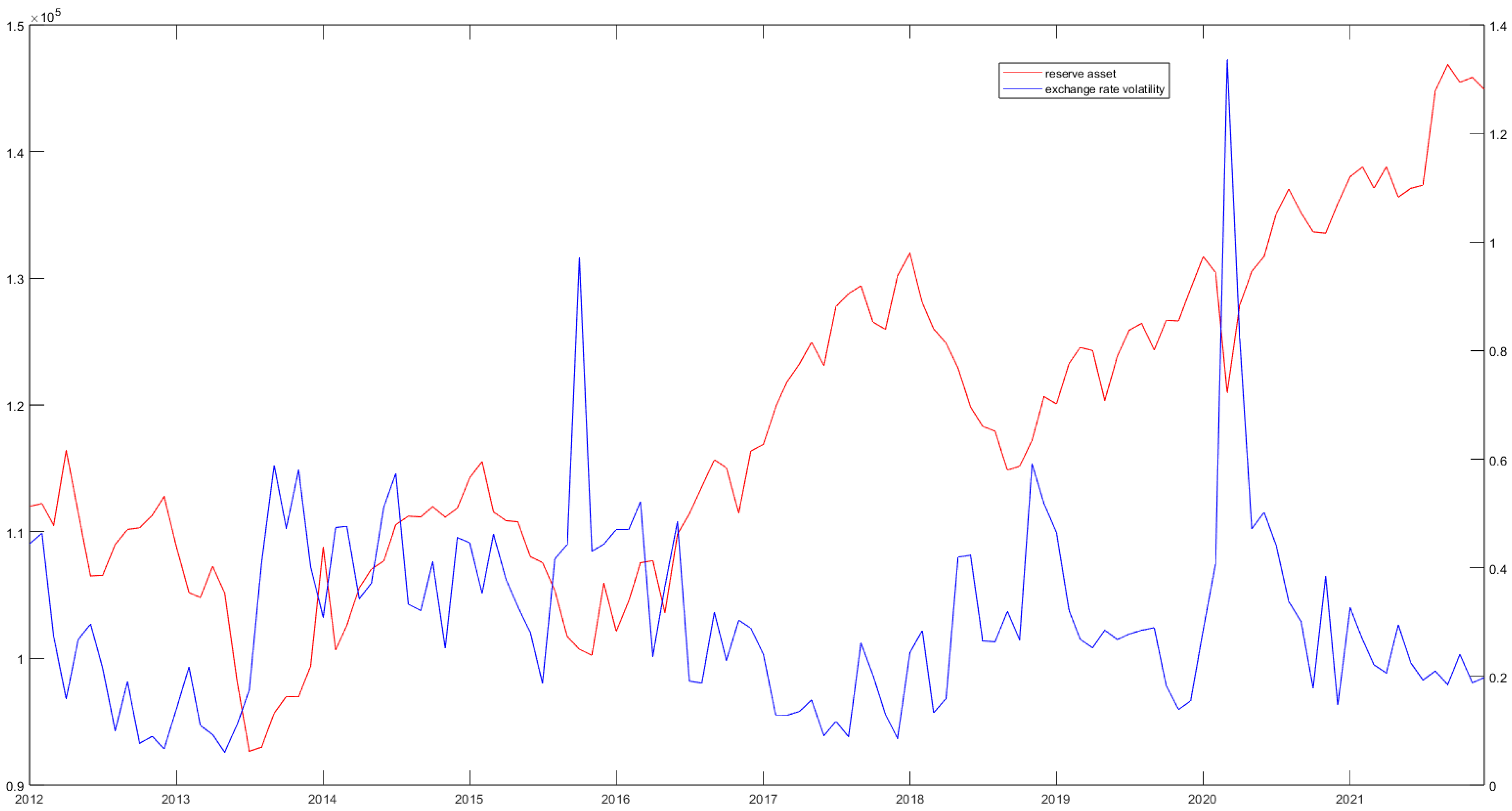
4.1. Exchange Rate Volatilities

Figure 1 illustrates the stochastic volatility of the exchange rate, displaying the mean alongside the upper and lower bounds of one standard deviation. Notably, spikes in volatility are observed at various points, corresponding to global financial market fluctuations and the COVID-19 pandemic. The highest volatility peak after the introduction of the export proceeds repatriation policy aligns with the prolonged effects of the COVID-19 pandemic.

To analyze the impact of export proceeds on exchange rate volatility, we selected eight specific dates summarized in

Table 1. Dates for sampling.

Date	Stochastic Volatility	Volatility Category
19 March 2020	2.1511	High
24 March 2020	1.7044	High
9 October 2015	1.6520	High
4 August 2014	0.5966	Mid
20 June 2018	0.4082	Mid
11 July 2016	0.2032	Mid
7 June 2017	0.0880	Low
24 October 2012	0.0748	Low

, capturing three of the highest volatility peaks, two of the lowest volatility points, and three dates with mid-range volatility levels after the enforcement of the policy. This selection is based on exchange rate volatility data from 2008 onward, incorporating the period that influenced the introduction of the export proceeds repatriation requirement in response to the currency instability triggered by the 2008 Global Financial Crisis. This selection provides deeper insights into the relationship between export proceeds and exchange rate volatility, particularly in response to policy motivations rooted in historical currency crises.

4.2. Estimation Results

Table 2. Estimation results of selected parameters in the TVP-VAR model.

Parameter	Mean	Stdev	95 Percent Interval	GCD	Inefficiency
${\left({\Sigma }_B\right)}_1$	0.000008	0.000001	[0.000006, 0.000010]	0.428	37.15
${\left({\Sigma }_B\right)}_2$	0.000666	0.000092	[0.000519, 0.000877]	0.946	39.04
${\left({\Sigma }_{\alpha }\right)}_1$	0.004377	0.003770	[0.001222, 0.015440]	0.026	181.57
${\left({\Sigma }_{\alpha }\right)}_2$	0.005944	0.003887	[0.001757, 0.016852]	0.002	176.33
${\left({\Sigma }_{\log \sigma }\right)}_1$	0.576859	0.057139	[0.472987, 0.697278]	0.427	26.92
${\left({\Sigma }_{\log \sigma }\right)}_2$	0.078714	0.013666	[0.054799, 0.108744]	0.701	64.28

Note: the estimates of $\left({\Sigma }_B\right)$ and $\left({\Sigma }_{\alpha }\right)$ are multiplied by 1000. The subscripts in the Parameter denote the number of sequence of parameters presented in the table.

presents the estimation results for the selected parameters. The results show that our MCMC algorithm produces posterior draws efficiently. The table provides the posterior means and standard deviations of the selected parameters, the Geweke Convergence Diagnostics (GCD) calculated following Geweke (1992), the 95% credible intervals, and the inefficiency factor. From Table 2, we find that the null hypothesis that the posterior distribution converges is not rejected at the 5% significance level on the basis of GCD statistics. Thus, the MCMC converges to a stationary distribution, and the estimates are stable. The inefficiency factors are quite low except for $\alpha$, the simultaneous relations of the structural shocks. This finding indicates that the convergence of the simultaneous relations is slow compared with that of other parameters. In sum, the MCMC sampler converges reliably and yields efficient posterior estimates, except that the simultaneous-shock coefficient $\alpha$ mixes more slowly than the other parameters.

4.3. Standard Deviation of Residuals

Figure 2 presents the posterior mean of the standard deviation of residuals for each equation in the TVP-VAR model. For most of the sample, these standard deviations remain low, indicating that the model captures the underlying dynamics well. Thus, the model performs well for all equations. However, several notable time points stand out where the standard deviations increase significantly; for example, on October 2015 and March 2020. The time points coincide with decreasing foreign exchange reserve assets and peak points of exchange rate volatility, as presented in Figure 3, suggesting central bank interventions during high exchange rate volatility periods. The model treats these interventions as unsystematic shocks, causing the larger residuals. In other words, when policy actions intensify during periods of stressed currency markets, the innovations in the TVP-VAR no longer fully explain the data, and the residual standard deviations increase accordingly.

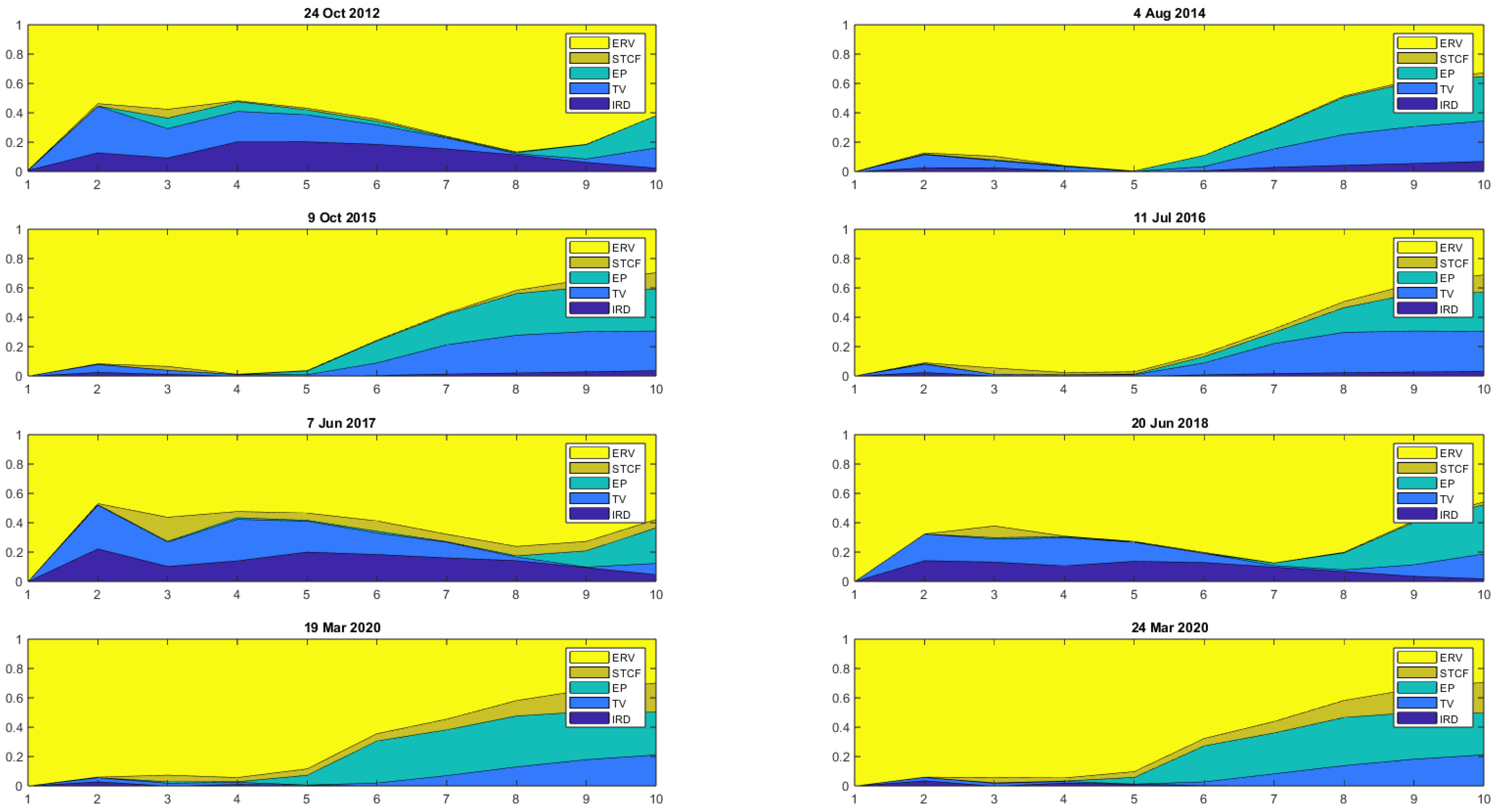
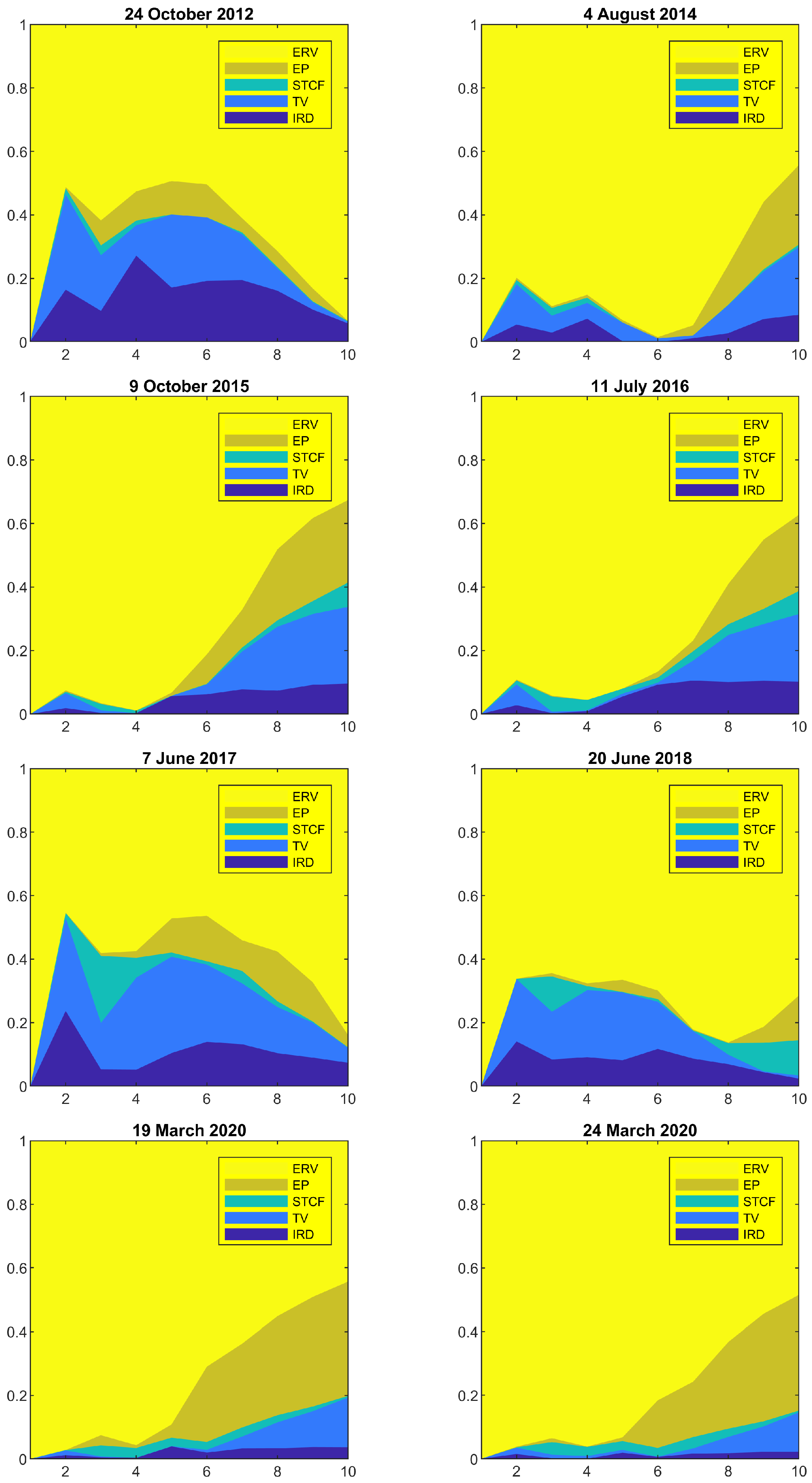
4.4. Forecast Error Variance Decomposition

The forecast error variance decomposition in Figure 4 demonstrates that, in the short run (1–2 horizons), ERV is predominantly driven by its own shocks, consistent with the findings of Meese and Rogoff (1983), Rossi (2013), De and Sun (2020), and Narayan (2022), inter alia. In the intermediate period (3–5 horizons), the influence of STCF begins to emerge, whereas EP becomes more prominent in the longer run (6–10 horizons). Notably, STCF contributions decrease as EP contributions increase over time.

These results suggest that neither EP nor STCF significantly impacts ERV in the short run. Moreover, the earlier influence of STCF, followed by the later prominence of EP, suggests that EP does not necessarily dampen the impact of STCF in the intermediate period.

In contrast to the existing literature, which highlights the negative impact of foreign exchange outflows on ERV (Caporale et al., 2017; Rafi & Ramachandran, 2018), our findings suggest that the magnitude of ERV does not appear to significantly influence the contributions of STCF or EP shocks to ERV. This observation implies the presence of other factor(s) that may affect ERV during periods of high volatility and dampen the effects of STCF and EP. Figure 3 shows a relationship between sharp declines in foreign exchange reserves and periods of elevated ERV, such as in October 2015 and March 2020. This suggests potential central bank interventions during these periods. Consequently, while EP and STCF may have short-term impacts on ERV, their impacts may be overshadowed by such interventions, potentially explaining the observed results. These findings also highlight that macro-fundamentals, most notably interest rate differentials, explain a far larger fraction of the ERV than EP or STCF.

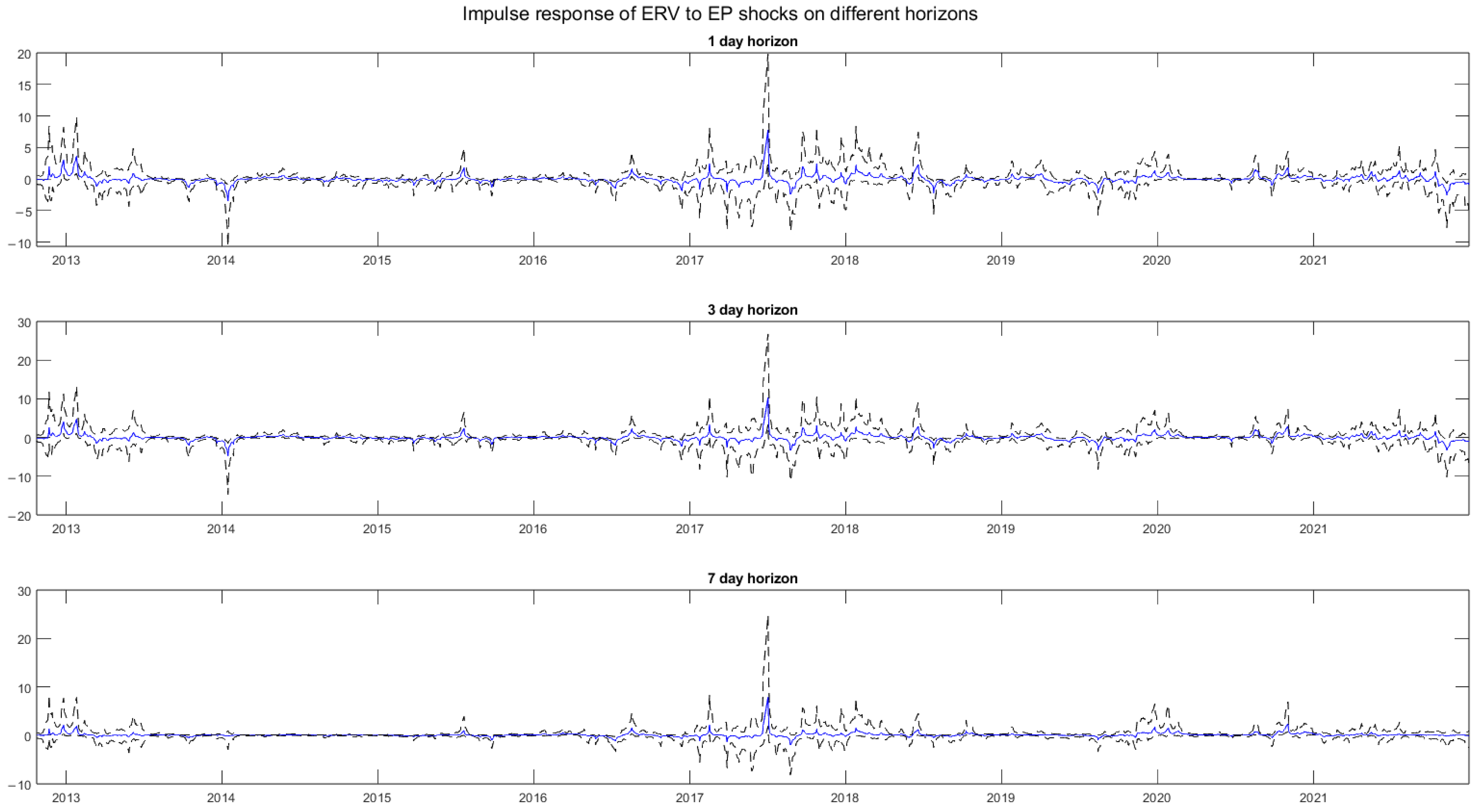
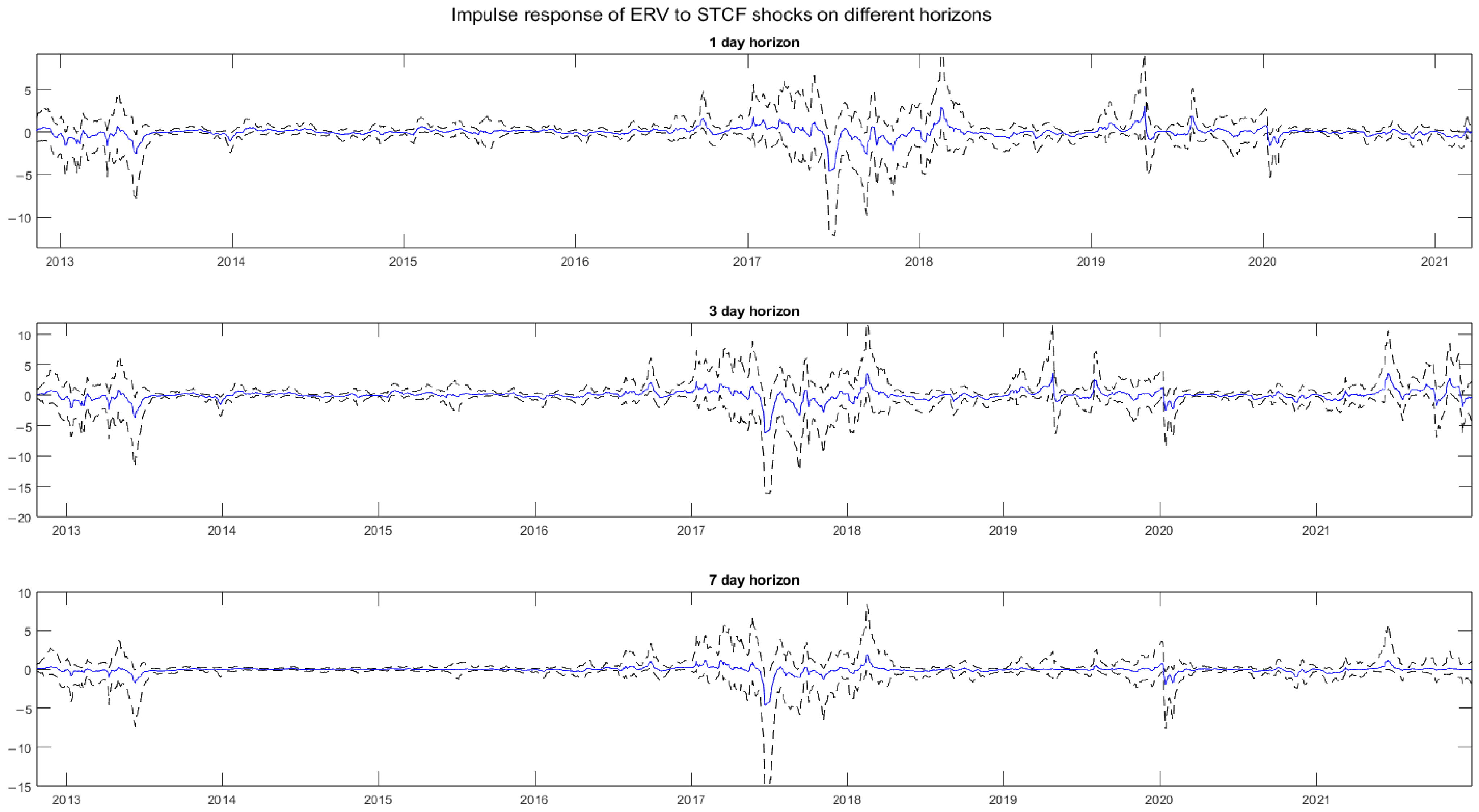
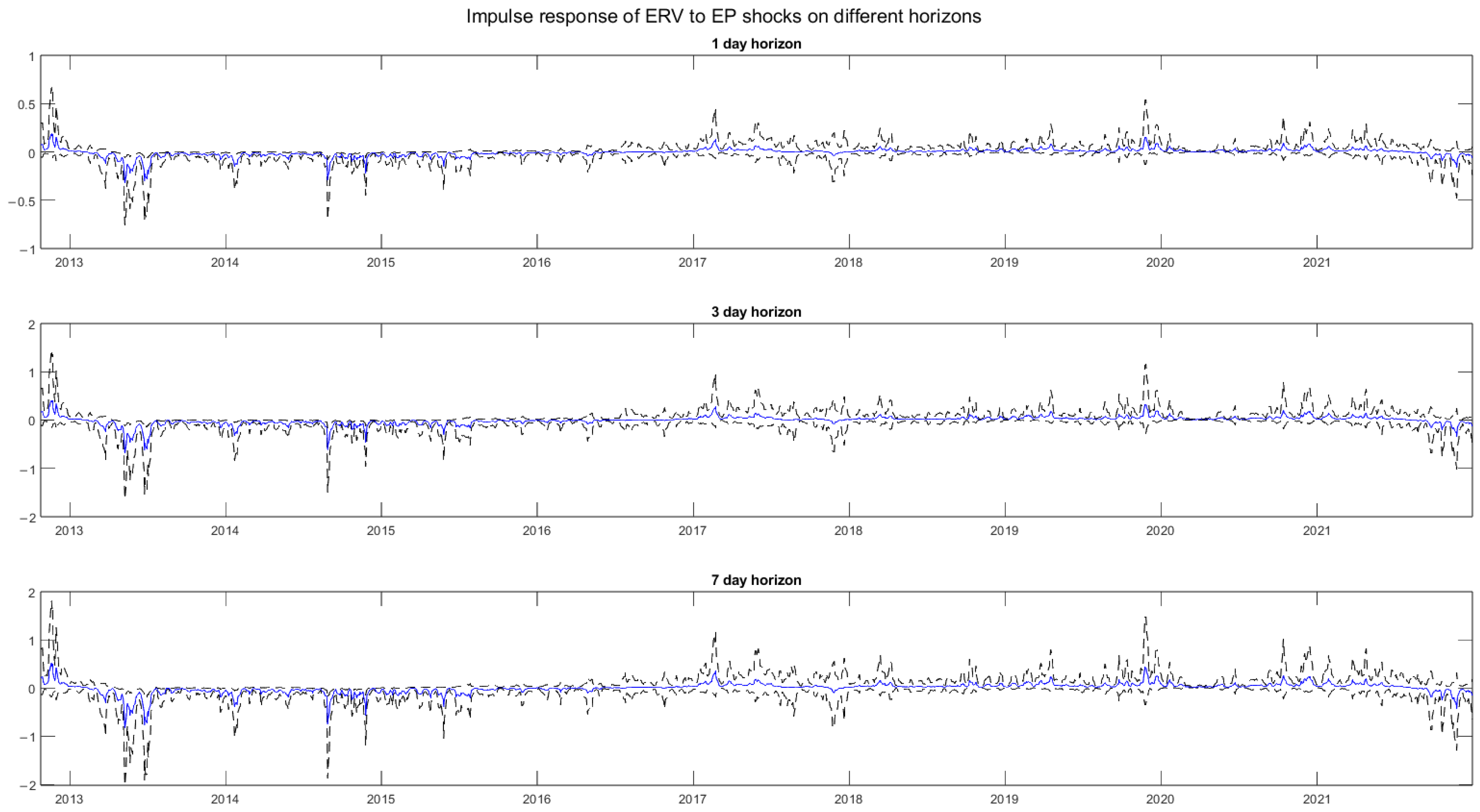
4.5. Impulse Response Functions

Figure 5 and Figure 6 present the ERV responses to STCF and EP shocks, respectively, on the sample dates. Both figures show that the responses vary significantly across the different dates, reflecting the time-varying nature of the relationship between ERV responses to STCF and EP shocks, as expected, with the TVP-VAR model’s ability to capture changing dynamics over time. There is also no evidence of patterns that differentiate the ERV responses to STCF or EP shocks between periods of high, medium, or low ERV periods. This observation is also shown in ERV responses to all variables’ shocks on sample dates in Figure 7. As discussed above, there are indications of central bank interventions during high volatility periods. Thus, the ERV responses during those periods may have been dampened by the interventions.

The responses of ERV to STCF shocks on sample dates, as presented by Figure 5, are mostly flat around zero for all horizons. The results are also statistically significant across all dates, indicating a consistent impact of STCF on all horizons. On the other hand, Figure 6 presents the responses of ERV to EP shocks on sample dates, where, while they are also mostly flat around zero, they are not statistically significant for the high volatility dates as detailed in Table 1 (9 October 2015, 19 March 2020, 24 March 2020). This finding indicates that, during high volatility, EP might not have a strong or consistent impact on ERV.

An observation of the response on all dates of observation in Figure 8 reveals that the impact of STCF shocks on ERV during the period leading up to 2017 remained relatively stable around the zero mark. Moreover, from 2017–2018, there were more pronounced negative deviations. The negative response is expected, which is more consistent with the literature (Caporale et al., 2017; Rafi & Ramachandran, 2018) rather than flat responses. Post-2018, the dynamics appeared to have shifted into more positive impacts and became significantly larger during certain periods, most notably in March and April 2019 and in 2021, coinciding with the beginning of the COVID-19 pandemic outbreak and the slowing economic growth thereafter. This finding also suggests a noteworthy shift in the influence of STCF on exchange rate volatility, as confirmed by the variance decomposition in Figure 4. This is the opposite of what we expected from the literature. On the longer horizon, the ERV responses tend to resurge, but they are also associated with wider credible intervals, indicating greater uncertainty in the responses.

Conversely, Figure 9 reveals that the influence of EP shocks on ERV was predominantly negative until 2015. This trend manifested itself in several instances of notably more significant negative impacts over the long term. It indicates the effectiveness of the repatriated export proceeds policy in controlling ERV in the first several years of the enforcement of the policy. Post-2015, the dynamics appeared to have shifted. The effects of EP shocks on exchange rate volatility have transitioned mainly to being flat around zero with wider credible intervals, again indicating greater uncertainty in the responses. On the longer horizon, although ERV responses are moving in the same directions as in the short run, they are slightly larger, indicating that ERV reacts to EP faster than to STCF, which is quite the opposite of what we expected from the literature (Enders, 2015; Narayan, 2022). Finally, Figure 10 presents the responses of ERV for all sample dates on 1, 3, and 7-day horizons.

We also split the IRF between crisis (high latent volatility) and calm (low latent volatility) periods in order to highlight the importance of using a time-varying model. A constant-parameter VAR produces a single unconditional IRF; by construction, it cannot tell us what the shock does specifically on high-volatility days. The TVP-SV-VAR retains the full sample yet allows coefficients and innovation variances to adapt each day, so we can average the resulting ${\Sigma }_t$ in Equation (2) over any stress tier (high and low) and obtain truly state-contingent impulse responses. In other words, because the TVP-VAR lets both coefficients and error variances change from day to day, we can group those daily responses by stress level. That flexibility yields impulse responses that are genuinely state-dependent.

The differences matter for crisis-vs-calm analysis for several reasons. First, crisis periods often have different pass-through elasticities. Fixed parameters can only report the average effect, masking regime shifts. Second, high-volatility days come with fatter error variance; fixed-VAR standard errors are either biased (if we ignore heteroskedasticity) or inflated (if you correct heteroskedasticity). Finally, a crisis-average IRF able to say what will happen when volatility is already high while fixed-VAR cannot answer that because its IRF is unconditional.

Figure 11 and Figure 12 make visible what a single fixed-parameter VAR would hide. The two solid lines in the upper panel of Figure 11 track the average IRF of ERV to EP shock for high latent volatility days and low latent volatility days. Their paths diverge, converge, and even swap sign. The lower panel shows these differences oscillate between gains (days 3–5) and losses of (day 4), then surge again on day 9. A fixed VAR estimates one unconditional coefficient set; its IRF would be a single damped line lying somewhere inside the shaded bands, unable to display these sign-reversals or late-horizon surges. The blue 68 % band is narrowest when volatility is already high (day 1) and widens as shocks propagate; the red band does the opposite. Such horizon-by-state width is produced automatically because the TVP-SV-VAR lets the innovation variances evolve. A fixed VAR’s homoskedastic band would be either too tight in crises or too loose in calm periods, blurring significance. Based on these results, desk economists will be able to adjust intervention strategy daily. The interpretations are that, on very tranquil days, the EP shock can briefly raise volatility while, on stressed days, the same shock increasingly dampens volatility, cutting ERV after about two weeks (day 9). A fixed VAR’s average response would miss these regime-specific effects and could mis-signal when the export-receipt rule is most—or least—effective.

For STCF shocks, Figure 12 also shows that the TVP-VAR uncovers a pattern that a fixed VAR cannot: the response of exchange-rate volatility is virtually state-neutral in the first three days, diverges modestly on day 4, and then reverses sharply by day 10, for the low latent volatility regime while the high latent volatility regime remains flat. These results are also useful for daily intervention strategy. In stressed conditions, a short-term capital inflow amplifies volatility quickly but the effect is short-lived. Thus, the regulator should be prepared to lean against the wind around day 4 (e.g., sterilized sales or swap facility). In tranquil markets, the same inflow is quiet at first, then triggers a delayed volatility bump roughly ten trading days later. In this condition, the regulator should keep monitoring through the second calendar week; the late spike can catch the desk off-guard if liquidity has already been unwound.

In Appendix E, we present the IRFs of STCF and EP shocks on ERV when the horizon is wider (20 days). The figures demonstrate that the effect dies out and bands explode in longer horizons. Credible bands grow wider because shocks are propagated through the companion matrix. Eventually, the band becomes so wide that the IRFs are statistically indistinguishable from zero. Hence, our choice of horizon 10 above is validated.

5. Robustness Analysis

Robustness exercises are provided for our model through (i) different ordering of variables (IRD, TV, EP, STCF, ERV), (ii) change of priors, and (iii) change in lag structure (p = 4). For our first robustness check, we change the ordering of the variables in the TVP-VAR setup. As our hypothesis in our model is that EP is more exogenous than STCF is, in this robustness check, we switch the ordering of STCF and EP to see whether it affects our results. We found that the results are consistent with our model, as shown by the variance decomposition in Figure A3.

Furthermore, we change the priors to flat priors. To ensure a consistent comparison of the results, we use the same dataset as our original model, where the first 200 days were excluded since they were used to calibrate the priors. The results for EP and STCF shocks on ERV are consistent with our model, as presented by Figure A4, Figure A5 and Figure A6. Our last robustness test involves changing the number of the lag structure to 4. The results are also consistent with our model and are presented in Figure A7, Figure A8 and Figure A9 (all figures are available in the appendixes). Therefore, we conclude that our model demonstrates robustness across all conducted sensitivity and robustness checks.

6. Conclusions

In this paper, we investigate the impact of short-term capital flows and repatriated export proceeds on exchange rate volatility in Indonesia from 1 January 2012 to 31 December 2021. We also examine whether repatriated export proceeds can act as a buffer for the effect of short-term capital flows on exchange rate volatility.

Overall, when measured relative to the long-term mean, the magnitude of the impact stemming from shocks in repatriated export proceeds on exchange rate volatility is less pronounced than that of shocks from short-term capital flows, although it varies significantly over time. This disparity in the scale of the two types of shocks underscores the possibility that they play different roles in influencing exchange rate volatility in Indonesia.

We find that, in the short term (1–2 days), neither repatriated export proceeds nor short-term capital flows significantly impact exchange rate volatility. Our results also show that, in the intermediate term (3–5 days), repatriated export proceeds do not necessarily dampen the impact of short-term capital flows. However, in the longer term, EP seems to be able to influence exchange rate volatility more than short-term capital flows do in the longer term (6–10 days). An analysis of the difference between the impacts of repatriated export proceeds and short-term capital flows during periods of high and low volatility did not yield a conclusive result. During periods of high volatility, repatriated export proceeds do not have a strong or consistent impact on exchange rate volatility. Our results also indicate that the policy of repatriated export proceeds was effective in controlling exchange rate volatility in the first several years following its enforcement. However, after 2015, there was no evidence of the impact of repatriated export proceeds on exchange rate volatility. Thus, our findings suggest that there is ample room for improvement in the policy, especially concerning the duration for which repatriated export proceeds should be retained in the country.

However, since Indonesia is committed to maintaining an open-capital-account regime, imposing a mandatory minimum holding period on export earnings is unlikely to be viable. Instead, policy-makers should focus on market-based measures that encourage exporters to keep their foreign-exchange proceeds onshore. Strengthening domestic hedging and liquidity options—particularly by deepening swap and forward markets—would provide exporters with attractive, risk-management-oriented incentives to hold their receipts locally, thereby supporting exchange-rate stability without resorting to restrictive capital controls. In a broader sense, Panggabean et al. (2025) study the implementation of export proceeds repatriation policies in countries that include those that apply surrender and conversion to local currency requirements. The findings are parallel with ours in which the impact of export proceeds repatriation policies on exchange rate volatility is limited to shorter horizon only, albeit longer than our results. It finds that the impact is up to one year after the policy is first introduced or re-introduced, underscoring the possible impact of minimum holding period or conversion to local currencies.

Furthermore, given the proprietary nature of export proceeds data, future research on this topic across other emerging economies implementing export repatriation policies would be highly valuable. Expanding the empirical evidence in this area could offer deeper insights into the broader applicability and effectiveness of such policies in stabilizing exchange rate volatility across diverse economic contexts. Further research suggestions include incorporating central bank intervention since, during high volatility, the central bank tends to intervene, which may dampen the effect of export proceeds on exchange rate volatility.

References

1. Aghion, P., Bacchetta, P., Rancière, R., & Rogoff, K. (2009). Exchange rate volatility and productivity growth: The role of financial development. Journal of Monetary Economics, 56(4), 494–513. [Google Scholar] [CrossRef]
2. Alanya, W., & Rodríguez, G. (2018). Stochastic volatility in the Peruvian stock market and exchange rate returns: A bayesian approximation. Journal of Emerging Market Finance, 17(3), 354–385. [Google Scholar] [CrossRef]
3. Asiedu, E., & Lien, D. (2004). Capital controls and foreign direct investment. World Development, 32, 479–490. [Google Scholar] [CrossRef]
4. Aysun, U. (2024). Identifying the external and internal drivers of exchange rate volatility in small open economies. Emerging Markets Review, 58, 101085. [Google Scholar] [CrossRef]
5. Baum, C. F., & Caglayan, M. (2010). On the sensitivity of the volume and volatility of bilateral trade flows to exchange rate uncertainty. Journal of International Money and Finance, 29(1), 79–93. [Google Scholar] [CrossRef]
6. Bush, G., & López Noria, G. (2021). Uncertainty and exchange rate volatility: Evidence from Mexico. International Review of Economics and Finance, 75, 704–722. [Google Scholar] [CrossRef]
7. Caporale, G. M., Ali, F. M., Spagnolo, F., & Spagnolo, N. (2017). International portfolio flows and exchange rate volatility in emerging Asian markets. Journal of International Money and Finance, 76, 1–15. [Google Scholar] [CrossRef]
8. Carnero, M. A., Pena, D., & Ruiz, E. (2004). Persistence and kurtosis in GARCH and stochastic volatility models. Journal of Financial Econometrics, 2(2), 319–342. [Google Scholar] [CrossRef]
9. Chan, J., Koop, G., Poirier, D. J., & Tobias, J. L. (2019). Time series models for volatility. In Bayesian econometric methods (pp. 391–410). Cambridge University Press. [Google Scholar] [CrossRef]
10. Choudhri, E. U., & Hakura, D. S. (2006). Exchange rate pass-through to domestic prices: Does the inflationary environment matter? Journal of International Money and Finance, 25(4), 614–639. [Google Scholar] [CrossRef]
11. Clarida, R., & Gali, J. (1994). Sources of real exchange-rate fluctuations: How important are nominal shocks? Carnegie-Rochester Confer. Series on Public Policy, 41, 1–56. [Google Scholar] [CrossRef]
12. Daníelsson, J. (1998). Multivariate stochastic volatility models: Estimation and a comparison with VGARCH models. Journal of Empirical Finance, 5(2), 155–173. [Google Scholar] [CrossRef]
13. De, K., & Sun, W. (2020). Is the exchange rate a shock absorber or a source of shocks? Evidence from the U.S. Economic Modelling, 89, 1–9. [Google Scholar] [CrossRef]
14. Devereux, M. B., & Engel, C. (2002). Exchange rate pass-through, exchange rate volatility, and exchange rate disconnect. Journal of Monetary Economics, 49, 913–940. [Google Scholar] [CrossRef]
15. Dominguez, K. M., & Frankel, J. A. (1993). Does foreign-exchange intervention matter? The portfolio effect. American Economic Review, 83(5), 1356–1369. [Google Scholar]
16. Eichenbaum, M., & Evans, C. L. (1995). Some empirical evidence on the effects of shocks to monetary policy on exchange rates. The Quarterly Journal of Economics, 110(4), 975–1009. [Google Scholar] [CrossRef]
17. Enders, W. (2015). Applied econometrics time series (4th ed., Vol. 19). John Wiley and Sons, Inc. [Google Scholar]
18. Feldmann, H. (2011). The unemployment effect of exchange rate volatility in industrial countries. Economics Letters, 111(3), 268–271. [Google Scholar] [CrossRef]
19. Flood, R. P., & Rose, A. K. (1999). Understanding exchange rate volatility without the contrivance of macroeconomics. The Economic Journal, 109(459), F660–F672. [Google Scholar] [CrossRef]
20. Fuller, W. A. (1996). Introduction to statistical time series: Second edition. John Wiley and Sons, Incorporated. [Google Scholar] [CrossRef]
21. Gabaix, X., & Maggiori, M. (2015). International liquidity and exchange rate dynamics. The Quarterly Journal of Economics, 130(3), 1369–1420. [Google Scholar] [CrossRef]
22. Geweke, J. (1992). Evaluating the accuracy of sampling-based approaches to the calculation of posterior moments. In J. M. Bernardo, J. Berger, P. Dawid, & A. F. M. Smith (Eds.), Bayesian statistics 4: Proceedings of the fourth Valencia international meeting, dedicated to the memory of Morris H. DeGroot, 1931–1989 (pp. 169–193). Oxford University Press. [Google Scholar] [CrossRef]
23. Grier, R., & Grier, K. B. (2006). On the real effects of inflation and inflation uncertainty in Mexico. Journal of Development Economics, 80(2), 478–500. [Google Scholar] [CrossRef]
24. Grossmann, A., & Orlov, A. G. (2014). A panel-regression investigation of exchange rate volatility. International Journal of Finance and Economics, 326, 303–326. [Google Scholar] [CrossRef]
25. Guillaumont, P. (1980). The impact of declining terms of trade and inflation on the export proceeds and debt burden of developing countries. World Development, 8, 763–768. [Google Scholar] [CrossRef]
26. Hafner, C. M., & Preminger, A. (2010). Deciding between GARCH and stochastic volatility via strong decision rules. Journal of Statistical Planning and Inference, 140(3), 791–805. [Google Scholar] [CrossRef]
27. Jacquier, E., Polson, N. G., & Rossi, P. E. (1994). Bayesian analysis of stochastic volatility models. Journal of Business and Economic Statistics, 12(4), 69–87. [Google Scholar] [CrossRef]
28. Kim, S., Shephard, N., & Chib, S. (1998). Stochastic volatility: Likelihood inference and comparison with ARCH models. Review of Economic Studies, 65(3), 361–393. [Google Scholar] [CrossRef]
29. Krol, R. (2014). Economic policy uncertainty and exchange rate volatility. International Finance, 17(2), 241–256. [Google Scholar] [CrossRef]
30. Lane, P. R. (2001). The new open economy macroeconomics: A survey. Journal of International Economics, 54(2), 235–266. [Google Scholar] [CrossRef]
31. Lee-Lee, C., & Hui-Boon, T. (2007). Macroeconomic factors of exchange rate volatility: Evidence from four neighbouring ASEAN economies. Studies in Economics and Finance, 24(4), 266–285. [Google Scholar] [CrossRef]
32. Macbean, A. I. (1962). Causes of excessive fluctuations in export proceeds of underdeveloped countries. Bulletin of the Oxford University Institute of Economics & Statistics, 27, 323–341. [Google Scholar] [CrossRef]
33. Massell, B. F. (1964). Export concentration and fluctuations in export earnings: A cross-section analysis. The American Economic Review, 54, 47–63. [Google Scholar]
34. Meese, R., & Rogoff, K. S. (1983). Empirical exchange rate models of the seventies: Do they fit out of sample? Journal of International Economics, 14(1–2), 3–24. [Google Scholar] [CrossRef]
35. Morimune, K. (2007). Volatility models. Japanese Economic Review, 58(1), 1–23. [Google Scholar] [CrossRef]
36. Nakajima, J. (2011). Time-varying parameter VAR model with stochastic volatility: An overview of methodology and empirical applications. Monetary and Economic Studies, 29, 107–142. [Google Scholar]
37. Narayan, P. K. (2022). Understanding exchange rate shocks during COVID-19. Finance Research Letters, 45, 102181. [Google Scholar] [CrossRef] [PubMed]
38. Negro, M. D., & Primiceri, G. E. (2015). Time varying structural vector autoregressions and monetary policy: A corrigendum. Review of Economic Studies, 82(4), 1342–1345. [Google Scholar] [CrossRef]
39. Panggabean, S., Ekananda, M., Gitaharie, B. Y., & Djuranovik, L. (2025). Export proceeds repatriation policies: A shield against exchange rate volatility in emerging markets? arXiv, arXiv:2506.09168. [Google Scholar] [CrossRef]
40. Pitt, M. K., & Shephard, N. (1999). Filtering via simulation: Auxiliary particle filters. Journal of the American Statistical Association, 94(446), 590–599. [Google Scholar] [CrossRef]
41. Powell, A. A. (1959). Export receipts and expansion in the wool industry. Australian Journal of Agricultural Economics, 3, 64–74. [Google Scholar] [CrossRef]
42. Prayoga, D. S., & Purnomo, D. (2024). The influence of foreign exchange policy from export proceeds, import payments, inflation rate, and rupiah exchange rate on foreign direct investment in Indonesia. Indonesian Interdisciplinary Journal of Sharia Economics (IIJSE), 7, 4875–4901. [Google Scholar]
43. Primiceri, G. E. (2005). Time varying structural vector autoregressions and monetary policy. Review of Economic Studies, 72(3), 821–852. [Google Scholar] [CrossRef]
44. Rafi, O. P. C. M., & Ramachandran, M. (2018). Capital flows and exchange rate volatility: Experience of emerging economies. Indian Economic Review, 53(1), 183–205. [Google Scholar] [CrossRef]
45. Reinhart, C. M., & Reinhart, V. R. (2009). Capital flow bonanzas: An encompassing view of the past and present. NBER International Seminar on Macroeconomics, 5(1), 9–62. [Google Scholar] [CrossRef]
46. Rossi, B. (2013). Exchange rate predictability. Journal of Economic Literature, 51, 1063–1119. [Google Scholar] [CrossRef]
47. Ulm, M., & Hambuckers, J. (2022). Do interest rate differentials drive the volatility of exchange rates? Evidence from an extended stochastic volatility model. Journal of Empirical Finance, 65, 125–148. [Google Scholar] [CrossRef]
48. Wallich, H. C. (1961). Stabilization of proceeds from raw material exports. In H. S. Ellis, & H. C. Wallich (Eds.), Economic development for latin america (pp. 342–365). Palgrave Macmillan UK. [Google Scholar] [CrossRef]
Figure 1. Posterior means of the time-varying stochastic volatility of the USD/IDR daily exchange rate returns data from 2008 to 2021. Note: The horizontal solid red line represents the mean volatility level, while the horizontal dashed red lines indicate the upper and lower bounds of one standard deviation. The vertical solid blue line marks the introduction of the export proceeds repatriation policy.
Economies 13 00180 g001
Figure 2. Posterior means of the standard deviation of residuals for each equation in the TVP-VAR model.
Economies 13 00180 g002
Figure 3. Foreign exchange reserve asset vs. mean of daily exchange rate volatility.
Economies 13 00180 g003
Figure 4. Forecast error variance decomposition of the TVP-VAR equations on sample dates.
Economies 13 00180 g004
Figure 5. Impulse response of exchange rate volatility to a 1% increase in short-term capital flows where the dashed lines denote the 16th and 84th percentiles on sample dates.
Economies 13 00180 g005
Figure 6. Impulse response of exchange rate volatility to a 1% increase in export proceeds where the dashed lines denote 16th and 84th percentiles on sample dates.
Economies 13 00180 g006
Figure 7. Impulse responses of exchange rate volatility on several dates.
Economies 13 00180 g007
Figure 8. Impulse response of exchange rate volatility to a 1% increase in short-term capital flows (blue line) while the black lines denote 16th and 84th percentiles.
Economies 13 00180 g008
Figure 9. Impulse response of exchange rate volatility to a 1% increase in export proceeds (blue line) while the black lines denote 16th and 84th percentiles.
Economies 13 00180 g009
Figure 10. Impulse responses of exchange rate volatility for all sample dates on 1-, 3-, and 7-day horizons.
Economies 13 00180 g010
Figure 11. Impulse response of exchange rate volatility to export proceeds shocks in crisis vs. calm periods.
Economies 13 00180 g011
Figure 12. Impulse response of exchange rate volatility to short-term capital flows shocks in crisis vs. calm periods.
Economies 13 00180 g012