Article

Empirical Investigation of the Sources of Inflation in Sri Lanka: Assessing the Roles of Global and Domestic Drivers

by
E. M. Ekanayake
1,* and
P. M. A. L. Dissanayake
2
1
College of Business and Entrepreneurship, Bethune-Cookman University, 640 Dr. Mary McLeod Bethune Blvd., Daytona Beach, FL 32114, USA
2
Department of Economics, University of Colombo, Colombo 03, Sri Lanka
*
Author to whom correspondence should be addressed.
Economies 2025, 13(4), 102; https://doi.org/10.3390/economies13040102
Submission received: 20 January 2025 / Revised: 31 March 2025 / Accepted: 31 March 2025 / Published: 2 April 2025
(This article belongs to the Section Macroeconomics, Monetary Economics, and Financial Markets)

Abstract

:
The annual inflation rate in Sri Lanka accelerated to record levels in recent years, especially after the COVID-19 pandemic. Though the inflation rate had declined to pre-pandemic levels by mid-2024, it is of great importance to identify the factors that caused hyperinflation during the COVID-19 pandemic. The objective of this study is to investigate the drivers of inflation in Sri Lanka using a structural vector autoregressive model and a multiple regression model. The study assesses both the global drivers and the domestic drivers of inflation. The study uses monthly data on the inflation rate, global oil price, exchange rate, policy rate, the global supply chain pressure index, and unemployment rate, covering the period from January 2020 to August 2024, focusing on the period of rapid increase in the inflation rate in Sri Lanka. The empirical results of the study provide evidence to conclude that the inflation rate in Sri Lanka during the 2020–2024 period was mainly driven by the growth rates in money supply, exchange rates, and global supply chain disruptions. The results also show that the volatility of the Sri Lanka inflation rate is mostly explained by the money supply and exchange rate movements in the long run.
JEL Classification:
E31; E52; F41

1. Introduction

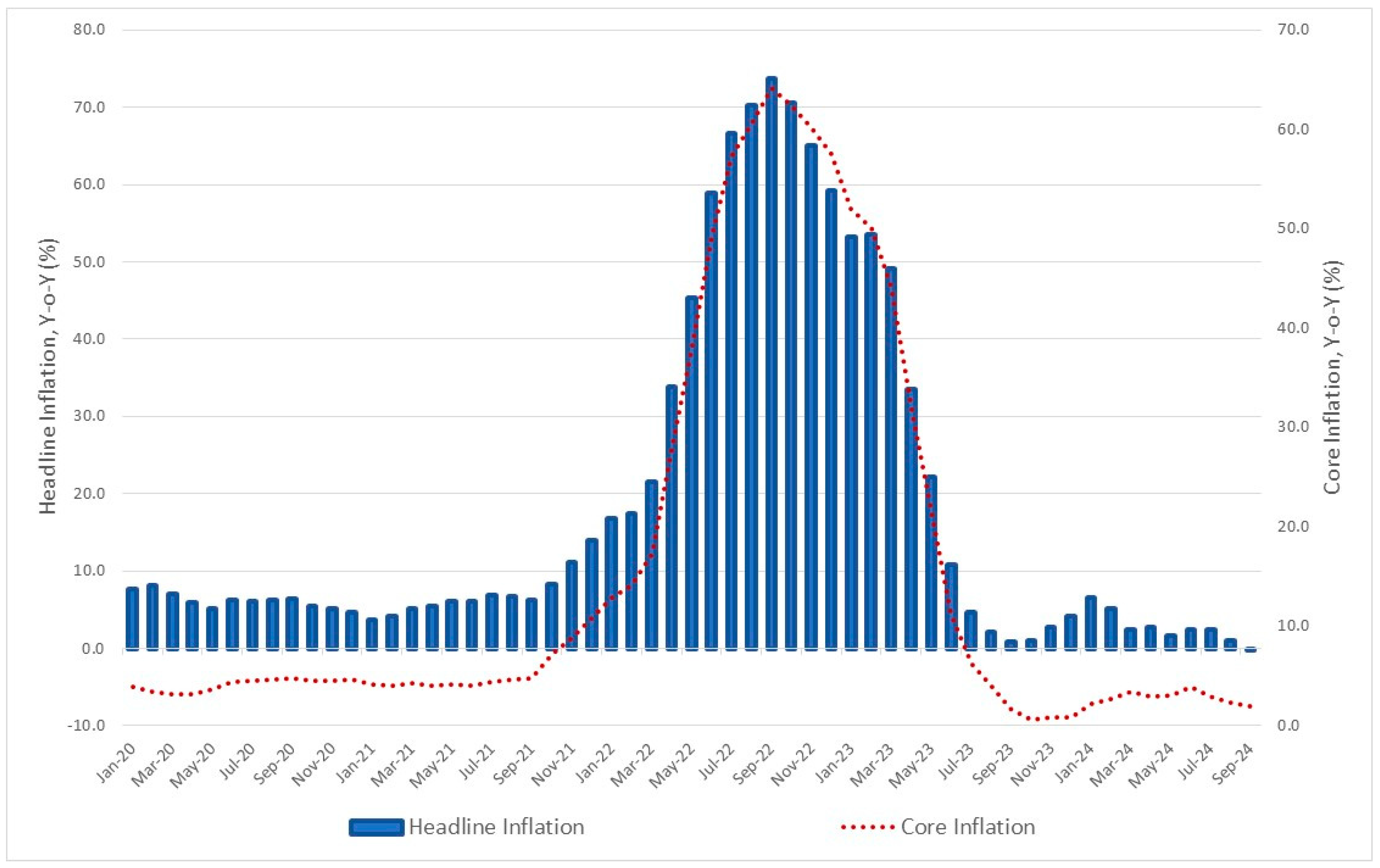
Sri Lanka was grappling with its worst financial crisis in seven decades because of economic mismanagement and the impact of the COVID-19 pandemic during the period from mid-2021 to mid-2023. According to the World Health Organization, most of the COVID-19 infections and deaths in Sri Lanka happened between October 2020 and March 2022 (see Figure 1). Though COVID-19 was not directly responsible for the rapid inflation in Sri Lanka, government policies that were used to combat COVID-19 during and after the pandemic played an important role. As Figure 2 illustrates, the annual inflation rate in Sri Lanka accelerated to record levels in recent years, especially after the COVID-19 pandemic. This episode of high inflation in Sri Lanka took place between October 2021 and June 2023, and it kept the inflation rate above 10%. As Figure 2 demonstrates, both the headline inflation and the core inflation remained above 10% between December 2021 and June 2023. Sri Lanka also experienced hyperinflation between June 2022 and March 2023, with the inflation rate remaining continuously above 50% during that period. According to the Department of Census and Statistics, Sri Lanka’s inflation rate, measured using the National Consumer Price Index (NCPI), rose to a peak of 73.6% in September 2022 on a year-on-year basis. Since then, the inflation rate declined gradually to reach 59.2% in December 2022. Disinflation continued throughout the year 2023 and the inflation rate dropped below 5% in July 2023, on a year-on-year basis.
However, there were signs of the inflation rate decreasing in 2023. According to the Central Bank of Sri Lanka, as measured by the year-on-year (Y-o-Y) change in the Colombo Consumer Price Index (CCPI, 2021 = 100), the inflation rate decreased to 35.3% in April 2023 from 50.3% in March 2023. The lower level of realized inflation compared to the projections made was mainly due to higher-than-expected price decreases observed in volatile food and non-food items. The food inflation (Y-o-Y) decreased to 30.6% in April 2023 from 47.6% in March 2023, while the non-food inflation (Y-o-Y) decreased to 37.6% in April 2023 from 51.7% in March 2023.
According to the Central Bank of Sri Lanka, looking ahead, based on the available information, the anticipated declining trend of inflation is expected to continue through 2024, bringing down the prevailing high inflation towards single-digit levels by late 2024. This disinflation process is supported by subdued aggregate demand owing to tight monetary and fiscal policy measures and the normalization of supply conditions both globally and domestically, along with the greater pass-through of lower global commodity prices.
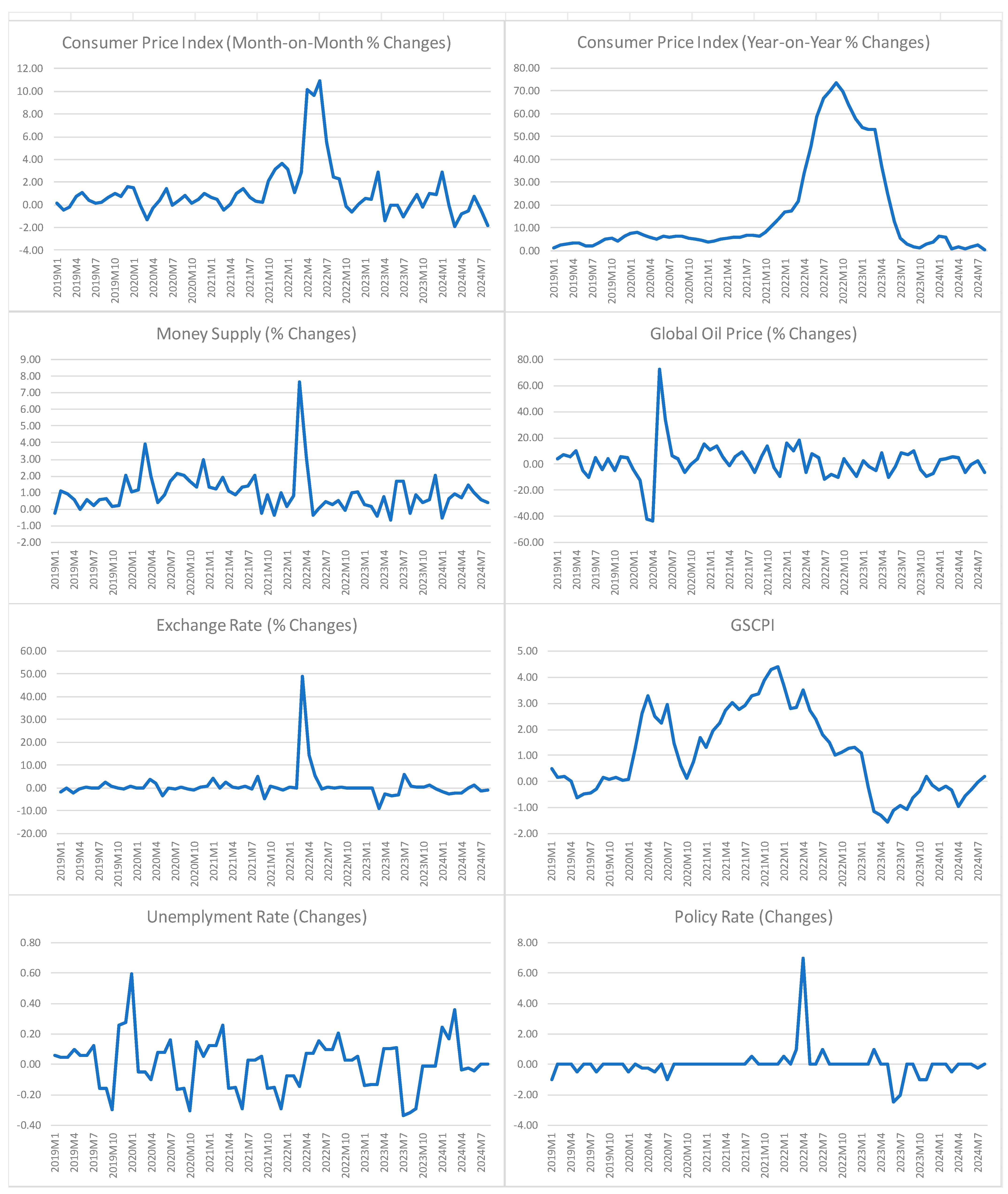
Given this rather unusual increase in inflation in Sri Lanka, identifying the triggers behind it is of great importance since it would help to decide on which measures to take to prevent the occurrence of similar episodes in the future. This study has identified several factors that may have contributed to rapid inflation in recent years. The recent trends of these factors are presented in Figure 3. The inflation rate measured by the year-on-year change in the CCPI reached a peak of 73.7% in September 2022 while the month-on-month change in the CCPI reached a peak of 10.9% in June 2022. These increases were followed by the money supply increasing by 7.6% and the nominal exchange rate depreciating by 48.7% in March 2022. The policy rate also increased from 6.5% in March 2022 to 13.5% in April 2022. The combination of these factors may have contributed to high inflation in 2022. The objective of this study s to investigate the both the global drivers and the domestic drivers of inflation in Sri Lanka.
In this paper, we contribute to the emerging empirical literature dealing with the causes of inflation during the COVID-19 pandemic focusing on a small open economy that depends heavily on imports of products, such as manufactured goods, petroleum, machinery, chemicals and related goods, and food. After this introductory section, the remaining sections of the paper are organized as follows: Section 2 presents a review of the literature while Section 3 presents the methodology and data sources. Section 4 presents empirical results and a discussion of the results. The main findings of the study are summarized and conclusions are drawn in Section 5.

2. Review of Literature

A significant body of literature can be found on the drivers of inflation. In this section, a summary of a wide variety of related recent studies is presented.
Congregado and Esteve (2022) studied the relationship between money growth and inflation in Spain using a classical inflation model with rational expectations. The study used data covering the period from 1830 to 1998 and employed cointegration analysis. The study found that ignoring the structural changes in the long-run cointegration relationships may understate the extent of the relationship between inflation rate and money growth.
Kilian and Zhou (2022) examined the persistence of inflationary effects resulting from gasoline price shocks, using monthly data for the U.S. from April 1990 to May 2022. The study used a structural vector autoregressive (SVAR) model and found no evidence that these effects are persistent, although the short-term impact on headline inflation is significant. However, gasoline price shocks accounted for only a small portion of overall inflation. In contrast, the study estimated that the effect on core personal consumption expenditure (PCE) inflation in 2022 and 2023 would be approximately 0.3 percentage points, already incorporating increases in inflation expectations.
Garzón and Hierro (2022) investigated the correlation between the euro/dollar exchange rate and oil prices, as well as its impact on the transmission of oil price fluctuations to headline inflation within the Euro area since the introduction of the common currency. The study used quarterly data for the Euro Area, the U.K., and Japan, spanning a period from 1999Q1 to 2019Q3. The study estimated an augmented Phillips curve that incorporated oil price changes to examine the role of the exchange rate in the oil price pass-through using multiple model specifications. The findings indicate a positive correlation between the euro/dollar exchange rate and oil prices, whereby an increase in oil prices led to an appreciation of the euro. Additionally, the study found that the appreciation of the euro partially mitigated the transmission of oil price fluctuations to the Euro area’s headline inflation.
Kantur and Özcan (2021) examined inflation dynamics during the COVID-19 pandemic, finding that inflation was higher than the official general inflation rate during the first lockdown, suggesting behavioral shifts in consumption patterns. Using credit and debit card transaction data from Turkey, the study constructed an alternative pandemic consumption basket price index from January 2020 to February 2021, incorporating revised Consumer Price Index (CPI) weights. The results indicate that consumption habits largely reverted to pre-pandemic patterns during the reopening period. Furthermore, the study found that the difference between pandemic-specific inflation and general inflation was less pronounced during the second lockdown compared to the first.
Bonam and Smădu (2021) analyzed historical pandemics and their long-term effects on trend inflation in Europe, using a historical dataset which covered the period 1313–2018 and an inflation series for six European countries: France (1387–2018), Germany (1326–2018), Italy (1314–2018), the Netherlands (1400–2018), Spain (1400–1729, 1800–2018), and the UK (1314–2018). The study found that past pandemics led to a significant decline in trend inflation lasting over a decade. However, the study suggests that the impact of COVID-19 on trend inflation may differ from previous pandemics.
Cochrane (2022) studied the fiscal roots of inflation using U.S. data for the period from 1947 to 2018. The study developed a set of linearized identities expressing the relationship between government debt, inflation, and fiscal surpluses. The study asserts that the real value of government debt equals the present value of real primary surpluses. The findings indicate that nominal government debt is devalued by higher inflation, and as a result, higher inflation corresponds to lower surplus-to-GDP ratios, slower GDP growth, and higher discount rates on government debt. Empirical analysis, based on vector autoregression and responses to recession, inflation, and fiscal shocks, showed that discount rates accounted for significant variation in inflation and the cyclical inflation pattern. Furthermore, the study found that long-term government bonds were gradually devalued by moderate inflation following fiscal shocks.
Bilici and Cekin (2020) analyzed inflation dynamics by estimating the persistence of inflation in Turkey from 1990 to 2018. Inflation persistence was defined as the speed at which inflation returns to its equilibrium level after a shock. The study applied a time-varying parameter estimation method based on the Kalman filter. The findings indicate that inflation persistence increased and exhibited high volatility during periods of high inflation, negatively impacting pricing behaviors and inflation expectations. Additionally, the study found that inflation began declining after 2003 and became less persistent following institutional changes in monetary policy. The monetary policy was effective in maintaining price stability until 2016. However, empirical results showed a considerable increase in inflation persistence from 2016 onward, coinciding with a rising inflation trend.
Jiang et al. (2022) examined the impact of the COVID-19 pandemic on inflation in China using online prices from 107 Chinese websites and the difference-in-differences method to exclude the effect of the Spring Festival. The study found that the pandemic led to a sudden 0.4% increase in the overall inflation rate, a 20% reduction in the probability of price changes, and a 1% reduction in the absolute price change size. The pandemic had heterogeneous effects across various sectors, causing significant structural changes in inflation. Price correction behaviors after the Spring Festival were disrupted, and whether products could be consumed while customers remained at home was a crucial factor affecting inflation dynamics and price adjustments.
A study by Elbahnasawy and Ellis (2022) investigated the relationship between inflation and e tstructure of economic and political systems using a wide range of political and economic structure variables. The study was based on a panel dataset of 156 countries covering the period from 1970 to 2009. The study found that both economic and political structures are important determinants of inflation. The study also found that a larger natural resource sector or a larger shadow economy was associated with higher inflation.
Alturki and Olson (2022) analyzed the impact of investor sentiment on the inflation premium in the United States. The study used daily data from 18 July 2008 to 31 August 2019. The study found that one standard deviation positive shock to general investor sentiment regarding oil prices leads to an approximate 1.2% increase in the inflation premium over the following 10 weeks. The analysis was conducted using a structural vector autoregressive (SVAR) model and out-of-sample forecasts. The findings indicate that institutional investor sentiment has a more pronounced effect on the inflation premium than individual investor sentiment. Additionally, the study provides out-of-sample evidence suggesting that the general investor sentiment regarding oil prices has predictive power over the U.S. inflation premium.
Arsić et al. (2022) examined the impact of inflation-targeting monetary frameworks on macroeconomic performance, utilizing data from 26 emerging economies in Europe and Central Asia between 1997 and 2019. The study employed propensity score matching and dynamic panel modeling for econometric analysis, measuring economic performance through inflation rates, inflation volatility, and GDP volatility. The findings suggest that inflation targeting has enhanced macroeconomic stability in these economies.
Mishra and Dubey (2022) investigated the spillover effects of the inflation-targeting monetary policy on financial stability in emerging market economies. Using data from 64 emerging markets for the period from 1998 to 2017, the study developed sector-specific stability and financial stability indices, employing dynamic panel data models within a difference-in-differences framework. The findings suggest that inflation targeting has significant positive spillover effects on banking system resilience and external capital inflows, driven by improved central bank accountability and transparency. The study recommends that emerging markets currently under an inflation-targeting lite regime transition to a full-fledged inflation-targeting framework.
Piergallini (2022) examined the dynamic implications of average inflation targeting within a tractable monetary framework featuring sticky prices. The study demonstrated that when a central bank assigns a relatively high weight to past inflation, average inflation targeting not only ensures local equilibrium determinacy but also effectively mitigates liquidity trap issues—contrasting with standard Taylor rules. Specifically, the study identified a saddle-path connection between the deflationary steady state and the target steady state, facilitating reflation through gradual and moderate increases in expected nominal interest rates.
Basse and Wegener (2022) analyzed the relationship between inflation expectations, interest rates, and inflation rates in Australia using monthly data from January 1995 to January 2019, testing for Granger causality. Empirical evidence from consumer surveys suggested that unidirectional Granger causality ran from medium- and long-term government bond yields to short-run inflation expectations. Additionally, bidirectional Granger causality was observed between short-term interest rates and short-run consumer inflation expectations. Sentimental data measuring inflation and interest rate expectations were found to be useful in forecasting inflation rates, with bond markets demonstrating high efficiency in this regard. The study further discussed issues related to traditional tests of the Fisher hypothesis and examined the role of financial deregulation in Australia, emphasizing the relevance of the Lucas critique in testing the Fisher effect.
Ooft et al. (2021) constructed annual inflation rate forecasts for Suriname using mixed data sampling regression, incorporating monthly inflation rates as explanatory variables. Given that monthly inflation data were available for only one and a half decades, the study focused on refining forecast accuracy. The constructed model was associated with a hybrid New Keynesian Phillips curve and demonstrated high accuracy, particularly during the high-inflation period of 2016–2017. Forecast performance improved significantly when data from May were included. Additionally, the study found that applying specific parameter restrictions further enhanced forecast accuracy.
Behera and Patra (2022) examined the concept of trend inflation, which represents the level to which actual inflation is expected to converge after short-term fluctuations subside. The study used quarterly data for India covering the period from 1980Q1 to 2019Q4. Their findings suggest that inflation expectations must align with trend inflation to prevent unanchored inflation expectations, a flattened aggregate supply curve, or the transmission of a deflationary bias to the economy. Using a regime-switching model applied to a hybrid New Keynesian Phillips curve, the study found a steady decline in trend inflation from 2014 to just before the onset of COVID-19, reaching 4.1–4.3%. Based on these results, the study recommended maintaining an inflation target of 4% for India.
Cruz (2022) investigated whether the decline in macroeconomic volatility following the adoption of inflation targeting was driven by shocks (impulses) or structural stability (propagation). Using quarterly data from both emerging (Thailand, Mexico, South Korea, the Philippines, and Indonesia for the period 1980Q1–2017Q4) and advanced economies (New Zealand, Canada, the United Kingdom, Sweden, and Australia for the period 1960Q1–2017Q4), the results indicate that the observed reduction in inflation variability was primarily attributable to the propagation mechanism (i.e., a more stable economic structure), while the reduction in output volatility was largely driven by smaller external shocks.
Han et al. (2022) developed a rational expectations framework to investigate the impact of information frictions and nominal rigidity on inflation and inflation beliefs. The study used U.S. data covering the period from 1968Q4 to 2019Q4. The study analytically derived a Phillips curve linking inflation, average inflation expectations, and the net effect of higher-order expectations. The results highlight the significant role of dispersed information in shaping inflation dynamics and forecast errors. The estimated impact of dispersed information explained a substantial share of inflation variability, while the net effect of higher-order expectations provided a novel micro foundation for markup shocks.
Dumitrescu et al. (2022) explored the nonlinear relationship between public debt and inflation using data from 22 emerging economies covering the 2006 to 2015 period. The study provided empirical evidence of threshold effects, indicating that economies with relatively low levels of shadow economic activity could accommodate higher public debt without incurring additional inflation-related welfare costs. However, in countries where the shadow economy exceeded 24.3% of GDP, public debt expansion was associated with significantly higher macroeconomic costs, including increased inflation. These findings suggest that such economies had limited policy flexibility in addressing the economic impact of the COVID-19 pandemic.
Doho et al. (2023) investigated the relationship between inflation and sectoral indices in West Africa from November 2001 to January 2020 using the asymmetric kernel method. The study analyzed indices in finance, retail, utilities, industry, transportation, agriculture, and other sectors. The results showed that the utilities and agriculture sectors were the most sensitive to inflation changes. A nonlinear relationship was identified between inflation and sectoral stock market indices, supporting the hypothesis that the correlation between inflation and stock market indices varies across different inflationary economies. The findings suggest that investors adjust their investment portfolios in response to inflation variations, ultimately impacting future dividends.
Hall et al. (2023) analyzed the recent drivers of inflation in three currency areas: the USA, the UK, and the Eurozone, using the data from 2000 to 2022. A vector autoregressive (VAR) model, Cholesky decomposition, and spatial modeling were used to identify the nature of inflationary shocks. The study found that inflationary shocks in the USA were strongly transmitted to the UK and the Eurozone. Additionally, the Eurozone transmitted inflationary pressures to a lesser extent, while inflation in the UK had minimal impact on the other two regions.
Makin et al. (2017) examined the relationship between inflation and excess currency growth in Australia. The study first reviewed the operation of monetary policy before analyzing how excess money supply growth, measured by M3 and currency, influenced inflation in Australia from 1970 to 2015 using various econometric techniques. The study also compared the pre- and post-inflation targeting periods. The results indicate that excess money growth was a key determinant of inflation in Australia, though its significance declined following the adoption of inflation targeting. The findings suggest that currency velocity, a fundamental component of the quantity theory of money, remained stable. Consequently, the study recommended that the role of excess currency growth in inflation should receive greater attention in monetary policy deliberations.
Chowdhury and Garg (2022) investigated whether the COVID-19 crisis strengthened the dynamic relationship between exchange rates and oil prices. The study was based on data for the period from 2 January 2017 to 10 August 2020, covering four countries, namely, China, India, Japan, and Korea. The study identified significant breaks in correlations, with a major structural break occurring around the pandemic outbreak. The results suggest that interactions between exchange rates and oil prices have increased post-pandemic. Policymakers and investors responded to the crisis by adjusting portfolios, favoring foreign currency-denominated assets when domestic currencies are depreciated.
While previous studies have employed various methodologies to analyze inflation drivers, this study utilizes a structural vector autoregressive (SVAR) model and multiple regression analysis to investigate the determinants of inflation in Sri Lanka. While the previous studies have focused on both developed and developing countries, there is no study that has investigated the causes of rapid inflation during the COVID-19 pandemic. In addition, none of the previous studies have used all methodologies employed in this study when investigating causes of inflation. This study fills the gaps in the literature by investigating the causes of inflation in Sri Lanka during the COVID-19 pandemic using three different types of methodologies.

3. Methodology and Data

3.1. Estimation Methodology

In this paper, we contribute to the emerging empirical literature dealing with the factors affecting inflation in Sri Lanka. The objective of this study is to investigate the drivers of inflation in Sri Lanka using a structural vector autoregressive model and a multiple regression model. The study assesses both the global drivers and domestic drivers of inflation. The study uses monthly data on inflation rates, global oil prices, exchange rates, money supply, unemployment rates, the global supply chain pressure index, and policy rates, covering the period from January 2020 to August 2024.
In order to formally investigate the drivers of inflation, first we utilize a structural vector autoregressive model (SVAR) with the following variables: inflation rate, global oil price, exchange rate, money supply, policy rate, the global supply chain pressure index, and unemployment rate. These variables were commonly used in studies on inflation. For example, global oil price was used in studies by Garzón and Hierro (2022), Alvarez et al. (2011), Alturki and Olson (2022), Sekine (2020), and Kilian and Zhou (2022); exchange rate was used in studies by Garzón and Hierro (2022), Hall et al. (2023), Ozdemir (2020), Diaz et al. (2024), and Valogo et al. (2023); money supply was used in studies by Correa and Lopes (2023), Hall et al. (2023), and Makin et al. (2017); policy rate was used in studies by Hall et al. (2023), and Yilmazkuday (2022); the global supply chain pressure index was used in studies by Diaz et al. (2024), and Gordon and Clark (2023); and unemployment rate was used in studies by Hall et al. (2023) and Yilmazkuday (2022). According to Chen et al. (2016), the SVAR model has advantages in analyzing dynamic relationships among relevant time sequence variables. The formal investigation is based on the following SVAR model:
A 0 x t = α + k = 1 9 A k x t k + ϑ t
where x t = ( i n f t , e x r t , o p t , m s t , p r t , s c t , u r t ) is a vector of seven variables, i n f t is the Sri Lankan inflation rate measured as the percentage change in the monthly Consumer Price Index (2010 = 100); e x r t is the percentage change in the monthly nominal exchange rate (Sri Lankan Rupees per U.S. Dollar); o p t is the percentage change in the monthly global oil price (U.S. Dollars per barrel); m s t is the percentage change in the monthly M2 money supply (Millions of Sri Lankan Rupees); p r t is the change in the monthly policy rate (percent); s c t is the change in the monthly global supply chain pressure index (percent); u r t is the change in the monthly unemployment rate (percent); α , A 0 , and A k are unknown coefficients and vectors to be estimated; and ϑ t is the vector of serially and mutually uncorrelated structural innovations.
Assuming that A 0 is reversible, for estimation purposes, the SVAR model is expressed in the reduced form as follows:
x t = b + k = 1 9 B k x t k + t
where b = A o 1 a , B k = A 0 1 A k for all k, and t = A 0 1 ϑ t is the vector of estimated residuals in the reduced form. The number of lags (of k = 9) has been determined by sequential modified LR test statistics (each test at 5% level), final prediction error, and Akaike information criterion.
In addition to the SVAR model, we also employ a multiple regression model to analyze the effects of factors affecting inflation in Sri Lanka using the following model:
I N F t = β 0 + β 1 E X R t + β 2 O P t + β 3 M S t 1 + β 4 P R t + β 5 S C t + β 6 U R t + ε t
where I N F t is the Sri Lankan monthly inflation rate, E X R t is the percentage change in the monthly nominal exchange rate (Sri Lankan Rupees per U.S. Dollar), O P t is the percentage change in the monthly oil price (U.S. Dollars per barrel), M S t 1 is the one period lag of the percentage change in the monthly M2 money supply (millions of Sri Lankan Rupees), P R t is the change in the monthly policy rate, S C t is the change in the monthly global supply chain pressure index, U R t is the change in the monthly unemployment rate, and ε t is an error term. The reason for including a lagged value of money supply is, as Figure 3 illustrates, because the peak in inflation rate occurred after the money supply reached its peak.
Due to the rapid increase in the inflation rate after 2019, both the SVAR model and the multiple regression model were analyzed for the 2020–2024 period. In addition, prior to the estimation of the models, unit-root tests and cointegration tests were performed. To check the stationarity of the variables we used two unit-root tests, namely, the augmented Dickey–Fuller (ADF) test (Dickey & Fuller, 1979) and the KPSS test (Kwiatkowski et al., 1992). The null hypothesis for the ADF test is H0: the variable has a unit root, while the null hypothesis for the KPSS test is H0: the variable is stationary. After testing for the presence of unit roots in each variable using the two tests, testing for cointegration among the variables included in the specified model (3) was conducted using the Johansen cointegration test (Johansen, 1988, 1991).

3.2. Data and Data Sources

The monthly data on money supply, unemployment rate, and policy rate are from the Central Bank of Sri Lanka online database (https://www.cbsl.lk/eresearch/) (accessed on 10 December 2024). The data on monthly exchange rates are from the International Monetary Fund, International Financial Statistics 2024 database (https://data.imf.org/) (accessed on 10 December 2024). The study uses the Europe Brent Spot Price FOB (Dollars per barrel) as the global oil price. The data on global oil prices are from the U.S. Department of Energy, Energy Information Administration (EIA) (https://www.eia.gov/) (accessed on 10 December 2024). Sri Lankan inflation rate was measured as the percentage change in the monthly Consumer Price Index (2010 = 100) and the data on CPI were obtained from the International Monetary Fund, International Financial Statistics 2024 database. The data on the global supply chain pressure index were obtained from the Federal Reserve Bank of New York (2024), Global Supply Chain Pressure Index, https://www.newyorkfed.org/research/gscpi.html (accessed on 10 December 2024).

4. Results and Discussions

4.1. Results of Variance Decomposition Analysis and Impulse Response Functions

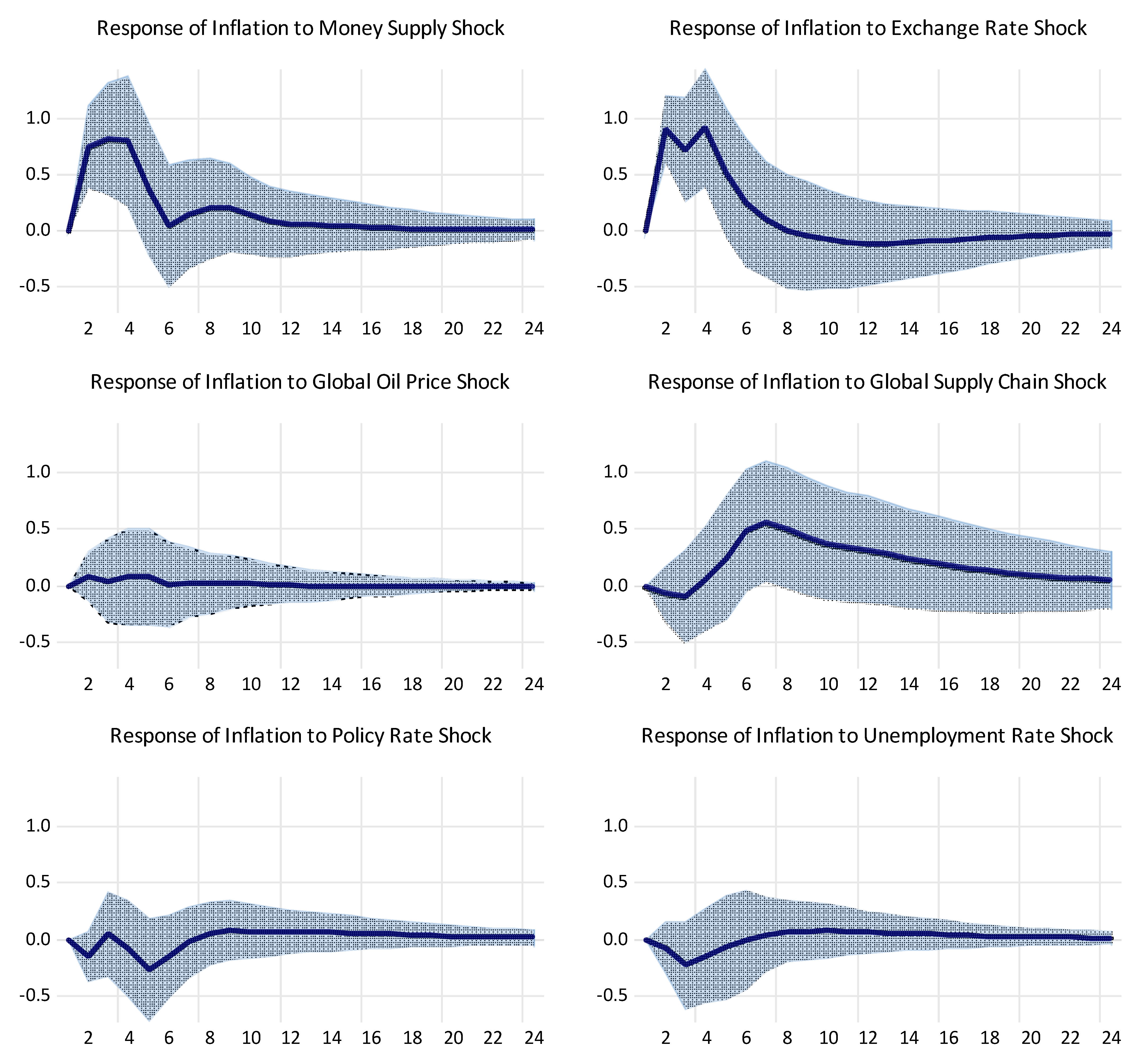
In this section, we discuss the results of the SVAR model, focusing on the relative contributions of these six types of structural innovations to inflation changes using the variance decomposition analysis and impulse response functions. This study focuses mainly on the high inflation period in Sri Lanka between 2020 and 2024. The extent of the fluctuations of inflation explained by innovations from each shock can be identified using a generalized forecast error variance decomposition analysis. Table 1 presents the summary of the contributions of various shocks to inflation in Sri Lanka during the period from January 2020 to August 2024. The accompanying impulse response function is presented in Figure 4.
The results of the variance decomposition analysis results presented in Table 1 show that the Sri Lankan inflation rate during the 2020–2024 period is mostly driven by the growth rate of money supply, the percentage change in the exchange rate, and the change in the global supply chain pressure index (followed by its own shock). These three drivers continued to be the most important force behind inflation even after two years of initial shocks. For example, in Month 7 they accounted for 75.3% of the variability in inflation rate and this share increased marginally to 78.6% in Month 24. The other three drivers, namely, the policy rate, global oil price, and unemployment, had very minor effects on the inflation rate, accounting for about 3% of the variability. Table 1 also shows that the effects of these shocks last only about six months in the case of money supply shock and about eight months in the case of the exchange rate. However, the effects of global supply chain disruptions last much longer. This is also evident from the impulse response functions presented in Figure 4. According to Figure 4, shocks to money supply, exchange rate, global supply chain disruptions, and global oil prices have positive effects on inflation in the first six to eight months, while shocks to the policy rate and unemployment rate have negative effects on inflation in the first six to eight months.
Based on the results discussed in this section, we can find evidence to conclude that the changes in the inflation rate in Sri Lanka were mainly driven by the growth rates in money supply, exchange rates, and global supply chain disruptions during the 2020–2024 period.

4.2. Unit-Root Tests and Cointegration Tests

Before estimating the multiple regression model specified in Equation (3), it is necessary to test the stationarity of the variables included in the model. The augmented Dickey–Fuller (ADF) test (Dickey & Fuller, 1979) and the KPSS test (Kwiatkowski et al., 1992) were used to check the stationarity of the variables. The null hypothesis for the ADF test is H0: the variable has a unit root, while the null hypothesis for the KPSS test is H0: the variable is stationary. The results of the unit-root tests are presented in Table 2. The results show that all variables, except the UR variable, are stationary at the first difference while the UR variable is stationary at the level.
After testing for the presence of unit roots in each variable, the next step involves testing for cointegration among the variables included in the specified model. For this purpose, we have used the Johansen cointegration test (Johansen, 1988, 1991).
The results of the Johansen cointegration test are presented in Table 3. The results presented in Table 3 reveal that both the Trace test and the Maximum Eigenvalues test indicate the existence of six cointegrating equations at the 5% level of significance. Thus, there is strong evidence to conclude that the seven variables included in Equation (3) are cointegrated or have a long-run relationship.

4.3. Regression Analysis

After testing the stationarity of the variables and the presence of a cointegrating relationship among the variables included in the multiple regression model specified in Equation (3), the model was estimated using four estimation methods, namely, the Ordinary Least Squares (OLS), the Fully Modified Least Squares (FMOLS), the Dynamic Least Squares (DOLS), and the Robust Least Squares (RLS). This allows us to check if the results are consistent among four estimation methods. The estimated results for the period from January 2020 to August 2024 are presented in Table 4.
The results presented in Table 4 show that the growth in the money supply variable has a positive effect on the inflation rate under four estimation methods. The estimated coefficient is also statistically significant at either a 1%, 5%, or 10% level of significance. The exchange rate variable has a positive effect on the inflation rate under all estimation methods, but the estimated coefficient is statistically significant only under the DOLS estimation method. The global oil price variable has a negative effect on the inflation rate under all estimation methods, but the estimated coefficient is not statistically significant under any estimation methods. The policy rate variable has a positive effect on the inflation rate under all estimation methods, and the estimated coefficient is statistically significant under all estimation methods. The global supply chain pressure variable also has a positive effect on the inflation rate under all estimation methods, and the estimated coefficient is statistically significant at the 1% level of significance under all estimation methods. The unemployment rate variable also has a negative effect on the inflation rate under all estimation methods, and the estimated coefficient is statistically significant at the 1% level of significance under all estimation methods. The results of the regression analysis for the period of January 2020 to August 2024 are consistent with those of the SVAR model.

4.4. Granger Causality Tests

In order to validate the results of the SVAR model and the regression analysis, this study also carried out Granger Causality Tests. The estimated results of the Granger Causality Test for the period from January 2020 to August 2024 are presented in Table 5.
The results presented in Table 5 show that there is a unidirectional causality running from money supply to inflation, exchange rate to inflation, the global supply chain pressure index to inflation, and policy rate to inflation, during the period from January 2020 to August 2024. Thus, the results of the Granger causality tests find evidence to claim that money supply, exchange rate, global supply chain pressure, and policy rate contributed to the inflation in Sri Lanka during the period from January 2020 to August 2024.

5. Conclusions

In this paper, we contribute to the emerging empirical literature dealing with the drivers of inflation in a small open economy. The objective of this study is to investigate the drivers of inflation in Sri Lanka using a structural vector autoregressive model and a multiple regression model. The study assesses both the global drivers and the domestic drivers of inflation. The study uses monthly data on inflation rates, global oil prices, exchange rates, money supply, unemployment rates, the global supply chain pressure index, and policy rates, covering the period from January 2020 to August 2024.
Based on the results of the SVAR model, we can find evidence to conclude that changes in the inflation rate in Sri Lanka were mainly driven by the growth rates in money supply, exchange rates, and global supply chain disruptions during the 2020–2024 period.
The results of the regression analysis suggest that the growth in money supply, growth rate of exchange rate, global supply chain pressure, and policy rate variables are the most important contributors to changes in the inflation rate during the 2020–2024 period. The results of the regression analysis for the period January 2020 to August 2024 are consistent with those of the SVAR model.
The results of the Granger causality tests show that there is a unidirectional causality running from money supply to inflation, exchange rate to inflation, the global supply chain pressure index to inflation, and policy rate to inflation, during the period from January 2020 to August 2024. Thus, we find evidence to claim that money supply, exchange rate, global supply chain pressure, and policy rate contributed to the inflation in Sri Lanka during the period from January 2020 to August 2024.
Consistent with the global impacts on inflation, previous studies (e.g., Jiang et al., 2022) emphasize that inflationary pressures are not just driven by domestic factors but are also significantly influenced by external disruptions, including global supply chain disruptions and exchange rate fluctuations. The link between money supply growth and inflation, as found in this study, mirrors findings from studies such as Makin et al. (2017), where excess money supply growth was identified as a key determinant of inflation. The impact of exchange rate fluctuations on inflation in Sri Lanka is consistent with findings from Chowdhury and Garg (2022), who identified significant shifts in inflation due to exchange rate movements, especially during periods of heightened economic uncertainty. The role of policy rates in controlling inflation, as observed in this study, aligns with the work of Basse and Wegener (2022), who found that short-term interest rate adjustments can significantly influence inflation expectations.
The findings of the study under three different statistical analyses used provide consistent results. The findings of the study show some important policy implications. In order to avoid a similar episode of high inflation, policymakers should not allow any rapid increase in the money supply. In addition, it is also equally important to maintain a relatively stable exchange rate.

Author Contributions

Conceptualization, E.M.E. and P.M.A.L.D.; methodology, E.M.E.; software, E.M.E.; validation, E.M.E. and P.M.A.L.D.; formal analysis, E.M.E.; investigation, E.M.E.; resources, E.M.E. and P.M.A.L.D.; data curation, E.M.E.; writing—original draft preparation, E.M.E. and P.M.A.L.D.; writing—review and editing, E.M.E. and P.M.A.L.D.; visualization, E.M.E. and P.M.A.L.D.; supervision, E.M.E.; project administration, E.M.E. All authors have read and agreed to the published version of the manuscript.

Funding

This research received no external funding.

Institutional Review Board Statement

Not applicable.

Informed Consent Statement

Not applicable.

Data Availability Statement

Data will be made available on request from the author.

Conflicts of Interest

The authors declare no conflicts of interest.

References

  1. Alturki, S., & Olson, E. (2022). Oil sentiment and the U.S. inflation premium. Energy Economics, 114, 1–13. [Google Scholar] [CrossRef]
  2. Alvarez, L. J., Hurtado, S., Sanchez, I., & Thomas, C. (2011). The impact of oil price changes on Spanish and Euro Area consumer price inflation. Economic Modelling, 28(1–2), 422–431. [Google Scholar] [CrossRef]
  3. Arsić, M., Mladenović, Z., & Nojković, A. (2022). Macroeconomic performance of inflation targeting in European and Asian emerging economies. Journal of Policy Modeling, 44(3), 675–700. [Google Scholar] [CrossRef]
  4. Basse, T., & Wegener, C. (2022). Inflation expectations: Australian consumer survey data versus the bond market. Journal of Economic Behavior and Organization, 203, 416–430. [Google Scholar] [CrossRef]
  5. Behera, H. K., & Patra, M. D. (2022). Measuring trend inflation in India. Journal of Asian Economics, 80, 1–13. [Google Scholar] [CrossRef]
  6. Bilici, B., & Cekin, S. E. (2020). Inflation persistence in Turkey: A TVP-estimation approach. The Quarterly Review of Economics and Finance, 78, 64–69. [Google Scholar] [CrossRef]
  7. Bonam, D., & Smădu, A. (2021). The long-run effects of pandemics on inflation: Will this time be different? Economics Letters, 208, 110065. [Google Scholar] [CrossRef] [PubMed]
  8. Chen, H., Lioa, H., Tang, B. J., & Wei, Y. M. (2016). Impacts of OPEC’s political risk on the international crude oil prices; an empirical analysis based on the SVAR models. Energy Economics, 57, 42–49. [Google Scholar] [CrossRef]
  9. Chowdhury, K. B., & Garg, B. (2022). Has COVID-19 intensified the oil price–exchange rate nexus? Economic Analysis and Policy, 76, 280–298. [Google Scholar] [CrossRef]
  10. Cochrane, J. H. (2022). The fiscal roots of inflation. Review of Economic Dynamics, 45, 22–40. [Google Scholar] [CrossRef]
  11. Congregado, E., & Esteve, V. (2022). Cointegration with structural changes and classical model of inflation in Spain, 1830–1998. Structural Change and Economic Dynamics, 60, 376–388. [Google Scholar] [CrossRef]
  12. Correa, W. L., & Lopes, L. S. (2023). Monetary policy transmission, productive activity, and inflation in Brazil: Does uncertainty matter? The Journal of Economic Asymmetries, 27, 1–17. [Google Scholar] [CrossRef]
  13. Cruz, C. J. (2022). Reduced macroeconomic volatility after adoption of inflation targeting: Impulses or propagation? International Review of Economics and Finance, 82, 759–770. [Google Scholar] [CrossRef]
  14. Diaz, E. M., Cunado, J., & de Garcia, F. P. (2024). Global drivers of inflation: The role of supply chain disruptions and commodity price shocks. Economic Modelling, 140, 106860. [Google Scholar] [CrossRef]
  15. Dickey, D. A., & Fuller, W. A. (1979). Distribution of the estimators for autoregressive time series with a unit root. Journal of American Statistical Association, 74(366), 427–431. [Google Scholar] [CrossRef]
  16. Doho, L. R., Some, S. M., & Banto, J. M. (2023). Inflation and West African sectoral stock price indices: An asymmetric kernel method analysis. Emerging Markets Review, 54, 1–15. [Google Scholar] [CrossRef]
  17. Dumitrescu, B. A., Kagitci, M., & Cepoi, C. O. (2022). Nonlinear effects of public debt on inflation. Does the size of the shadow economy matter? Finance Research Letters, 46, 102255. [Google Scholar] [CrossRef]
  18. Elbahnasawy, N. G., & Ellis, M. A. (2022). Inflation and the Structure of Economic and Political Systems. Structural Change and Economic Dynamics, 60, 59–74. [Google Scholar] [CrossRef]
  19. Federal Reserve Bank of New York. (2024). Global supply chain pressure index. Available online: https://www.newyorkfed.org/research/policy/gscpi (accessed on 10 December 2024).
  20. Garzón, A. J., & Hierro, L. A. (2022). Inflation, oil prices and exchange rates. The Euro’s dampening effect. Journal of Policy Modeling, 44, 130–146. [Google Scholar] [CrossRef]
  21. Gordon, M., & Clark, T. (2023). The impact of supply chain disruptions on inflation. Economics Commentary, EC 2023-08. [Google Scholar] [CrossRef]
  22. Granger, C. W. J. (1969). Some recent development in a concept of causality. Journal of Econometrics, 39(1–2), 199–211. [Google Scholar] [CrossRef]
  23. Granger, C. W. J. (1988). Investigating causal relations by econometric models and cross-spectral methods. Econometrica, 37, 424–438. [Google Scholar] [CrossRef]
  24. Hall, S. G., Tavlas, G. S., & Wang, Y. (2023). Drivers and spillover effects of inflation: The United States, the euro area, and the United Kingdom. Journal of International Money and Finance, 131, 102276. [Google Scholar] [CrossRef]
  25. Han, Z., Ma, X., & Mao, R. (2022). The role of dispersed information in inflation and inflation expectations. Review of Economic Dynamics, 48, 72–106. [Google Scholar] [CrossRef]
  26. Jiang, T., Liu, T., Tang, K., & Zeng, J. (2022). Online prices and inflation during the nationwide COVID-19 quarantine period: Evidence from 107 Chinese websites. Finance Research Letters, 19, 103166. [Google Scholar] [CrossRef]
  27. Johansen, S. (1988). Statistical analysis of cointegration vectors. Journal of Economic Dynamics and Control, 12(2–3), 231–254. [Google Scholar] [CrossRef]
  28. Johansen, S. (1991). Estimation and hypothesis testing of cointegration vectors in Gaussian vector autoregressive models. Econometrica, 59(6), 1551–1580. [Google Scholar] [CrossRef]
  29. Kantur, Z., & Özcan, G. (2021). What pandemic inflation tells: Old habits die hard. Economics Letters, 204, 109907. [Google Scholar] [CrossRef]
  30. Kilian, L., & Zhou, X. (2022). The impact of rising oil prices on U.S. inflation and inflation expectations in 2020–23. Energy Economics, 113, 106228. [Google Scholar] [CrossRef]
  31. Kwiatkowski, D., Phillips, P. C. B., Schmidt, P., & Shin, Y. (1992). Testing the null hypothesis of stationary against the alternative of a unit root. Journal of Econometrics, 54, 159–178. [Google Scholar] [CrossRef]
  32. MacKinnon, J. G., Haug, A. A., & Michelis, L. (1999). Numerical distribution functions of likelihood ratio tests for cointegration. Journal of Applied Econometrics, 14, 563–577. [Google Scholar]
  33. Makin, A. J., Robson, A., & Ratnasiri, S. (2017). Missing money found causing Australia’s inflation. Economic Modelling, 66, 156–162. [Google Scholar] [CrossRef]
  34. Mishra, A., & Dubey, A. (2022). Inflation targeting and its spillover effects on financial stability in emerging market economies. Journal of Policy Modeling, 44(6), 1198–1218. [Google Scholar] [CrossRef]
  35. Ooft, G., Bhaghoe, S., & Franses, P. H. (2021). Forecasting annual inflation in Suriname. Journal of International Financial Markets, Institutions & Money, 73, 101357. [Google Scholar] [CrossRef]
  36. Ozdemir, M. (2020). The role of exchange rate in inflation targeting: The case of Turkey. Applied Economics, 52(29), 3138–3152. [Google Scholar] [CrossRef]
  37. Piergallini, A. (2022). Average inflation targeting and macroeconomic stability. Economics Letters, 219, 110790. [Google Scholar] [CrossRef]
  38. Sekine, A. (2020). Oil price pass-through to consumer prices and the inflationary environment: A STAR approach. Applied Economic Letters, 27(6), 484–488. [Google Scholar] [CrossRef]
  39. Valogo, M. K., Duodu, E., Yusif, H., & Baidoo, S. T. (2023). Effect of exchange rate on inflation in the inflation targeting framework: Is the threshold level relevant? Research in Globalization, 6, 100119. [Google Scholar] [CrossRef]
  40. Yilmazkuday, H. (2022). Drivers of Turkish inflation. Quarterly Review of Economics and Finance, 84, 315–323. [Google Scholar] [CrossRef]
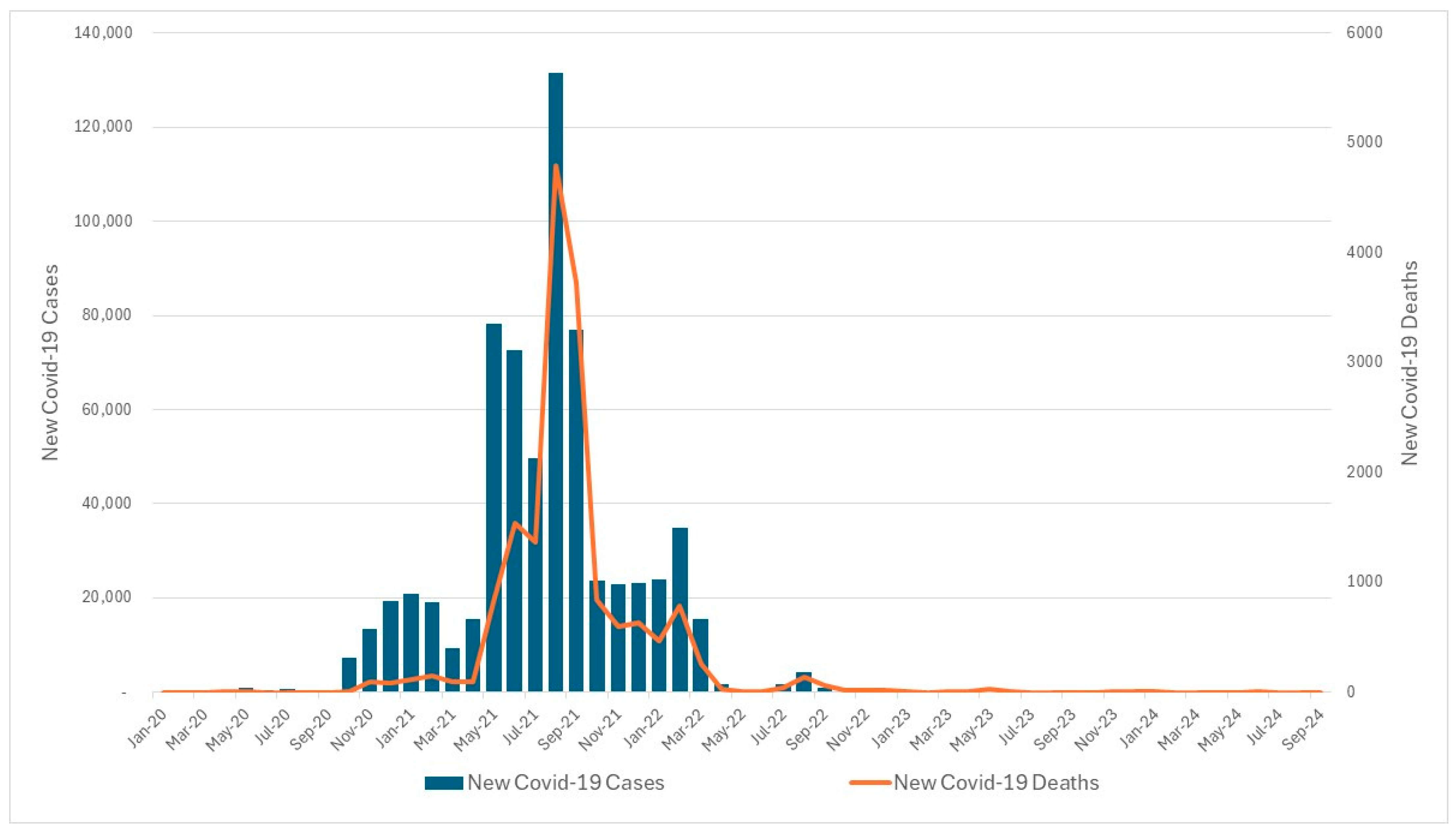
Figure 1. COVID-19 cases and deaths in Sri Lanka, 2020–2024. Note: The figure was constructed using the data from the World Health Organization (WHO).
Economies 13 00102 g001
Figure 2. Headline inflation and core inflation in Sri Lanka, 2020–2024. Note: The figure was constructed using data from the Central Bank of Sri Lanka. The inflation rates were calculated using the year-on-year (Y-o-Y) percentage change in the Colombo Consumer Price Index (2021 = 100).
Economies 13 00102 g002
Figure 3. Economic indicators that were used in the estimation. Note: The percentage of the National Consumer Price Index (month-on-month or year-on-year) was used as the rate of inflation. GSCPI represents the Global Supply Chain Pressure Index.
Economies 13 00102 g003
Figure 4. Impulse response functions. Sample Period: 2020M01–2024M08. Note: Response to Cholesky one S.D. (d.f. adjusted) innovations; 95% C.I. using analytic asymptotic standard errors.
Economies 13 00102 g004
Table 1. Contributions of various shocks to inflation rate (%). Sample period: 2020M01–2024M08.
MonthS.E.INFMSEXROPSCPRUR
10.988100.000.000.000.000.000.000.00
21.56849.9825.0921.950.201.311.250.21
31.88934.4433.5028.260.141.390.881.38
42.19725.5835.2535.530.211.190.711.53
52.30223.8434.1036.300.282.601.341.54
62.36922.7032.3435.050.276.611.521.51
72.43521.5730.9633.240.2611.071.461.44
82.49120.6930.0331.770.2514.471.401.38
92.53620.0629.3430.720.2416.881.391.36
102.57019.6128.7430.030.2418.631.401.36
112.59719.2528.2129.580.2419.931.421.37
122.61818.9727.7829.280.2320.921.441.38
132.63518.7527.4529.070.2321.651.471.38
142.64818.5827.1928.930.2322.181.501.39
152.65818.4527.0028.830.2322.561.521.40
162.66518.3626.8728.760.2322.841.541.41
172.67018.3026.7728.710.2323.031.551.42
182.67418.2526.7028.680.2323.171.561.42
192.67718.2126.6428.650.2323.271.571.42
202.67918.1926.6128.630.2323.351.571.42
212.68018.1726.5828.620.2323.411.581.43
222.68118.1626.5628.610.2323.451.581.43
232.68218.1526.5428.600.2323.481.581.43
242.68318.1426.5328.590.2323.501.591.43
Note: This table shows the variance decomposition of I N F using Cholesky (d.f. adjusted) factors for Cholesky one standard deviation (d.f. adjusted) innovations. Cholesky ordering: INF, MS, EXR, OP, SC, PR, and UR, where S.E. is the standard error, INF is the inflation rate, MS is the percentage change in money supply, EXR is the percentage change in the nominal exchange rate, OP is the percentage change in global oil price, SC is the change in global supply chain pressure index, PR is the change in policy rate, and UR is the change in the unemployment rate.
Table 2. Results of unit-root tests.
VariableADF TestKPSS Test
LevelDifferenceLevelDifference
CPI−1.044
(0.957)
−6.072 ***
(0.000)
0.280 ***0.069
MS−0.998
(0.941)
−11.207 ***
(0.000)
0.245 ***0.075
EXR−2.536
(0.310)
−9.676 ***
(0.000)
0.267 ***0.043
OP−2.212
(0.479)
−10.271 ***
(0.000)
0.244 ***0.057
PR−2.142
(0.518)
−10.554 ***
(0.000)
0.124 *0.046
SC−1.805
(0.692)
−8.042 ***
(0.000)
0.271 ***0.039
UR−3.421 *
(0.052)
−10.650 ***
(0.000)
0.1170.066
Note: C P I is the logarithm of the Sri Lankan monthly Consumer Price Index, E X R is the logarithm of the monthly nominal exchange rate, O P is the logarithm of the monthly oil price, M S is the logarithm of the monthly M2 money supply, P R is the logarithm of the monthly policy rate, S C is the logarithm of the monthly global supply chain pressure index, and U R is the logarithm of the monthly unemployment rate. Figures in parentheses are standard errors. A constant and a linear trend were included in all models. The null hypothesis for the ADF test is H0: the variable has a unit root. The null hypothesis for the KPSS test is H0: the variable is stationary. The asymptotic critical values of the KPSS test are 0.216, 0.146, and 0.119 for 1% level, 5% level, and 10% level, respectively. The asterisks *** and * represent the 1% and 10% levels of significance, respectively.
Table 3. Results of the Johansen cointegration test.
HypothesizedTrace TestMaximum Eigenvalues Test
No. of CE(s)Trace Statisticp-ValueMax. EV Statisticp-Value
r = 0226.27 ***0.000069.25 ***0.0000
r   1157.02 ***0.000052.16 ***0.0014
r   2104.86 ***0.000037.22 **0.0192
r   367.65 ***0.000329.20 **0.0307
r   438.44 ***0.004019.67 *0.0791
r   518.78 **0.015415.71 **0.0293
r 6 3.060.10083.060.1008
Note: This table presents the results of the Johansen cointegration tests. Figures in p-value columns are MacKinnon et al. (1999p-values and r is the hypothesized number of cointegrating equations. The asterisks ***, **, and * represent the statistical significance at the 1%, 5%, and 10% levels, respectively.
Table 4. Results of regression analysis (Sample period: 2020M01–2024M08). Dependent variable: I N F .
VariableOLSFMOLSDOLSRLS
C o n s t a n t 9.4292 ***
(0.001)
9.5430 ***
(0.000)
8.1902 ***
(0.002)
7.0378 ***
(0.001)
M S ( 1 ) 0.6901 **
(0.017)
0.9157 ***
(0.000)
0.2889 *
(0.071)
0.1921 *
(0.087)
E X R 0.0141
(0.511)
0.0117
(0.609)
0.2760 **
(0.013)
0.0125
(0.618)
O P −0.0171
(0.641)
−0.0163
(0.110)
−0.0161
(0.820)
−0.0099
(0.347)
P R 0.8972 ***
(0.000)
0.4400 ***
(0.005)
0.2399 *
(0.091)
0.9335 ***
(0.000)
S C 0.5414 ***
(0.001)
0.7548 ***
(0.000)
0.5569 ***
(0.002)
0.4186 ***
(0.000)
U R −2.7806 ***
(0.001)
−2.4995 ***
(0.000)
−2.0998 ***
(0.006)
−1.3986 ***
(0.001)
A d j u s t e d   R 2 0.57710.52390.89970.5870
N o .   o f   O b s e r v a t i o n s 56565556
Note: OLS stands for the Ordinary Least Squares; FMOLS stands for the Fully Modified Least Squares; DOLS stands for the Dynamic Least Squares; RLS stands for the Robust Least Squares. MS(−1) is a one-month lag of the percentage change in money supply, EXR is the percentage change in the nominal exchange rate, OP is the percentage change in global oil price, SC is the change in global supply chain pressure index, PR is the change in policy rate, and UR is the change in the unemployment rate. Figures in parentheses are standard errors. Asterisks ***, ** and * represent the statistical significance at the 1%, 5%, and 10% levels of significance, respectively.
Table 5. Results of the Granger causality test (Sample period: 2020M01–2024M08).
Null HypothesisNumber of
Observations
F-Statisticp-Value
MS does not Granger cause INF549.701 ***0.0003
INF does not Granger cause MS 0.4470.6419
EXR does not Granger cause INF5425.143 ***0.0000
INF does not Granger cause EXR 0.6500.5267
OP does not Granger cause INF540.2690.7654
INF does not Granger cause OP 1.9710.1502
SC does not Granger cause INF542.643 *0.0967
INF does not Granger cause SC 0.5100.6039
PR does not Granger cause INF543.274 **0.0463
INF does not Granger cause PR 0.5800.5638
UN does not Granger cause INF541.0430.3601
INF does not Granger cause UN 1.4930.2348
Note: This table shows the results of the Granger Causality test (Granger, 1969, 1988). INF is the inflation rate, MS is the percentage change in money supply, EXR is the percentage change in the nominal exchange rate, OP is the percentage change in global oil price, SC is the change in global supply chain pressure index, PR is the change in policy rate, and UR is the change in the unemployment rate. The asterisks ***, ** and * indicate the statistical significance of F-statistic at the 1%, 5%, and 10% levels of significance, respectively.
Disclaimer/Publisher’s Note: The statements, opinions and data contained in all publications are solely those of the individual author(s) and contributor(s) and not of MDPI and/or the editor(s). MDPI and/or the editor(s) disclaim responsibility for any injury to people or property resulting from any ideas, methods, instructions or products referred to in the content.