Article

A Game-Theoretic Analysis of the Coexistence and Competition Between Hard and Fiat Money

by
Kjell Hausken
* and
Guizhou Wang
Faculty of Science and Technology, University of Stavanger, 4036 Stavanger, Norway
*
Author to whom correspondence should be addressed.
Economies 2025, 13(3), 80; https://doi.org/10.3390/economies13030080
Submission received: 9 January 2025 / Revised: 27 February 2025 / Accepted: 4 March 2025 / Published: 19 March 2025
(This article belongs to the Special Issue The Political Economy of Money)

Abstract

:
This article presents a game-theoretic model analyzing the strategic competition between hard and fiat money, involving a representative player and a consolidated bank (including the central bank). The findings reveal counterintuitive interactions between inflation, interest rates, and monetary policy. When hard money becomes more favorable, through higher interest rates, lower transaction costs, or stronger preferences, the bank responds by withdrawing fiat money, reducing inflation but paradoxically lowering the player’s utility. Conversely, increasing the fiat money interest rate leads to money printing and inflation, benefiting both the player and the bank, but ultimately driving hard money out of existence. The model demonstrates how banks use selective fiat money printing and withdrawal to optimize their holdings at the expense of individual players. This study provides insights into currency competition, inflation control, and strategic monetary interventions, relevant for policymakers, financial institutions, and individuals navigating dual-currency economies. By analyzing 26 key parameters, the research uncovers both intuitive and unexpected economic dynamics, offering a structured approach to understanding the power of fiat money in shaping financial systems. These results highlight the importance of monetary policies, transaction costs, and interest rate adjustments in determining the long-term viability of competing monetary systems.

1. Introduction

Money is the cornerstone of modern economies, serving as a medium of exchange, unit of account, and store of value. Throughout history, various forms of money have emerged,1 each with its own attributes and economic implications. Hard money is defined as having a fixed supply, is scarce, decentralized, cannot be printed, and is difficult to counterfeit or manipulate. One approximate example is representative money (Nicholson, 1888, pp. 72–74; Steiner, 1941, p. 30) backed by and redeemable for gold. Gold and Bitcoin (Nakamoto, 2008) resemble hard money. Approximately 1% of additional gold was mined measured as year over year in the fourth quarter of 2024 (World Gold Council, 2024). Zimbabwe issues a gold-backed digital currency (Johnson, 2023). Approximately 1.8% of Bitcoin was mined per year in 2020–2024, slowly decreasing until the year 2140 when the Bitcoin supply will be fixed at 21 million. Hard money has a fixed supply, whether physical or digital.
Fiat money, relying on the government, is created and controlled by central authorities like central banks. That can cause inflation or deflation through money printing or withdrawal. Fiat money can be in physical or digital form, e.g., central bank digital currencies (CBDCs) and stablecoins, which are cryptocurrencies. Neither physical nor digital fiat money has a fixed supply. Central banks explore CBDCs to enhance fiat payment systems. Stablecoins are designed to maintain stable values relative to either fiat currencies, specific assets, or collections of assets.
This article’s research aim is to provide a game-theoretic analysis of how a representative player and a consolidated bank, consisting of a bank and a central bank, are impacted by the interplay between hard and fiat money. Two kinds of hard money are considered. For simplicity, we refer to the first kind as hard money, which we can think of as being resembled by Bitcoin, but can in principle be any kind of hard money. The second kind of hard money is gold. The two kinds of hard money differ in the interest rates earned from holding them, and the preferences of the player and bank for holding different types of money. These preferences differ since, e.g., Bitcoin and gold have different storage requirements, as well as differing in terms of accessibility, security, divisibility, portability, durability, regulation, centralization, volatility, environmental impact, etc. Only one kind of fiat money is considered.
Examples of research questions are as follows: How do the changes in the number of players impact loans and inflation? How do the changes in hard and fiat money interest rates impact the player’s borrowing and the bank’s fiat money printing/withdrawal? What impact do transaction costs have on the player’s consumption, assets holdings, borrowing, and utility? How do the preferences of the player and bank for holding different types of money impact the player’s and the bank’s strategic choices? How does hard money impact inflation? How do the player and the bank make strategic choices between hard and fiat money? In order to understand the interplay between hard and fiat money, this article takes the view that a broader account is needed of how hard and fiat money interact with consumption, borrowing, and other assets, rather than merely focusing narrowly on hard and fiat money which do not exist in a vacuum by themselves.
Since utility is generated in multiple ways, some of which may be absent, the utility function assumes independent contributions from each component, summing their effects rather than combining them multiplicatively. The player’s utility depends on its resource allocation into consumption and holding hard and fiat money, other assets, and gold, and its choices to incur hard and fiat money loans, i.e., six free-choice variables. The bank’s utility depends on its resource allocation into hard and fiat money and gold (separated out as an asset in this article), and whether to print or withdraw fiat money allocated to the player and the bank, which together with the player’s fiat money borrowing causes inflation or deflation, i.e., three free-choice variables.
The results are impacted by the bank’s fiat money printing and withdrawal, the interest rates on assets and borrowing, how the player and the bank value hard and fiat money holding and borrowing, assessed against consumption, and the different transaction costs for hard and fiat money for consumption and buying other assets and gold. A higher hard money interest rate or a higher utility exponent for hard money for the bank decreases inflation through the bank’s fiat money withdrawal, which benefits the bank but not the player. A higher utility exponent for hard money for the player also decreases inflation, but due to the bank’s money printing to compensate for the player’s decreased fiat money borrowing. That benefits both the player and the bank.
The article contributes to our understanding of the competition and coexistence between hard and fiat money. The impact of the changes of 26 parameter values is analyzed relative to a plausibly chosen benchmark. The increased interest rate for hard money benefits the bank, which holds more hard money and less gold, and withdraws fiat money, which decreases inflation. That, paradoxically, causes the player to hold less hard money and receive lower utility. However, the increased interest rate for fiat money benefits both the player and the bank due to fiat money printing. Inflation increases and hard money eventually disappears. That illustrates the bank’s power obtained by selective fiat money printing and withdrawal. Inflation increases when more printed fiat money is allocated to the player. The player benefits from both hard and fiat money and eventually borrows and holds less fiat money. The bank benefits from the player’s loans but not from decreased fiat money allocation. If the player obtains more resources, the bank withdraws fiat money. The player then borrows hard and fiat money, which benefits the bank. If the bank obtains more resources, the bank also prints fiat money. Both the player and the bank benefit and inflation decreases and levels out. These insights are beneficial for regulators and central banks seeking to determine how to adjust fiat money printing/withdrawal and inflation. For example, the findings indicate that increasing interest rates for fiat money can lead to inflationary pressures, while higher hard money interest rates stabilize inflation but may disadvantage consumers. The findings also have implications for how individuals, firms, banks, and other actors allocate their resources strategically in a hard and fiat money economy.
Section 2 provides a comprehensive review of the literature. Section 3 introduces the theoretical model, while Section 4 presents its analysis. Section 5 illustrates and interprets the model’s findings. Section 6 examines the role of prices within the model. Section 7 highlights key insights derived from the analysis. Section 8 outlines policy implications for central banks, followed by Section 9, which explores broader macroeconomic implications. Section 10 discusses the study’s limitations and potential directions for future research. Finally, Section 11 concludes the article.

2. Literature

A robust understanding of the existing literature is essential for positioning this study within the broader academic discourse. The literature on the competition and coexistence between hard and fiat money is diverse, encompassing various perspectives from monetary theory, financial economics, and game theory. To structure this review, the literature is categorized into eight thematic areas: (1) hard money, (2) cryptocurrencies and central bank digital currencies (CBDCs), (3) competition between fiat currencies, (4) competition between cryptocurrencies and fiat currencies, (5) algorithmic stablecoins and the blurring of monetary boundaries, (6) inflation and currencies, (7) transaction costs and currencies, and (8) game-theoretic analyses. This categorization facilitates a clearer analysis of the various dimensions influencing the dynamics of hard and fiat money and highlights relevant theoretical and empirical contributions that inform this study’s model.

2.1. Hard Money

Fisher (1920) emphasizes that “irredeemable paper money has consistently brought about adverse consequences for the nations employing it.” He continues that to avert relentless inflation, global economies need to adopt either commodity-based or hard money standards. Steiner (1941) provides early insights into the notion of representative money, backed by and redeemable for tangible assets like gold. Their contributions lay the foundation for understanding the inherent value of currencies rooted in physical resources. Cooper et al. (1982) highlight that the key driving force behind reestablishing the gold standard is the eradication of inflation and the establishment of a consistent non-inflationary economy. They propose a commodity standard that extends beyond gold, suggesting that such a standard will effectively stabilize overall price levels. Bordo and Vegh (2002) suggest that the mere existence of paper money is inadequate to put the inflationary process in motion. Hence, they do not agree with Juan Bautista Alberdi (1810–1884), one of the most influential economic and political thinkers of 19th-century Argentina, who contends that the act of introducing paper money would inevitably cause inflation and that this inflationary tendency would persist unless a hard money standard is restored. Ammous (2018) argues that people will gradually shift from using a national currency to adopting hard money, which better maintains its value over time. Examples of this evolution include primitive types of currency such as seashells, glass beads, iron, and copper, which were eventually superseded by gold and silver. Ammous and D’Andrea (2022) delve into the relationship between time preferences, fiat money, and hard money. They contend that fiat money will devalue over time due to inflation, and, conversely, that hard money such as Bitcoin can maintain its value over time. Hence, they argue, hard money diminishes uncertainty and fosters saving habits, and implementing a hard money standard has the potential to enhance elevated levels of societal progress. Long et al. (2021) examine the performance of Bitcoin and gold as safe-haven assets under different uncertainties using a nonlinear autoregressive distributed lag model. They show that gold can hedge against uncertainties better than Bitcoin. Boissay et al. (2022) study the fragmentation of cryptocurrencies due to the emergence of newer blockchains. Despite the absence of interoperability among different blockchains, they show that cryptocurrencies continue to demonstrate a strong correlation in terms of price movements and sustained growth due to speculative buying. Wen et al. (2022) compare the safe-haven properties of gold and Bitcoin during the COVID-19 pandemic using a time-varying parameter vector autoregression model. They argue that gold is a safe haven for oil and stock markets, and that Bitcoin cannot serve as a safe-haven asset. Fernández-Villaverde and Sanches (2023) introduce a micro-founded monetary model of a small open economy under the gold standard. They suggest that while the gold standard exposes the home country to short-term fluctuations in money, prices, and output due to external shocks, it provides long-term price stability, with the quantity of money and prices only temporarily deviating from their steady-state levels. This article explores the competition between hard and fiat money, assuming that fiat money is susceptible to inflation but has a lower transaction cost compared with hard money. The bank controls the fiat money supply, while the hard money supply remains fixed.

2.2. Cryptocurrencies and Central Bank Digital Currencies

In recent years, central banks have actively explored the potential of CBDCs to enhance monetary policy effectiveness, financial stability, and payment system efficiency. Kosse and Mattei (2023) highlight that 94% of surveyed central banks are now engaged in various stages of CBDC exploration, ranging from research to pilot programs, with a significant increase in experiments involving wholesale CBDCs. The study indicates that CBDCs could mitigate some of the volatility associated with cryptocurrencies, provide a more stable medium of exchange, and potentially challenge the role of privately issued digital currencies. These developments have important implications for the coexistence and competition between hard and fiat money, as analyzed in this article, by impacting inflation dynamics, financial inclusion, and the strategic behavior of central banks.
Nabilou (2020) highlights the potential risks associated with cryptocurrencies such as Bitcoin, which could challenge the monopoly held by central banks in money issuance. As a response, central banks delve into CBDCs. The author further points out that the European Central Bank faces legal obstacles that need to be addressed prior to CBDC’s introduction within the Eurozone. Adrian and Mancini-Griffoli (2021) investigate the emergence of digital money issued by private firms and central banks. They propose a synthetic CBDC that combines the advantages of private sector innovation with the safety and stability of central bank-backed money. Laboure et al. (2021) review the development of cryptocurrencies and CBDCs. They forecast a forthcoming coexistence between cryptocurrencies and traditional fiat money. They also emphasize the need to tackle various issues, e.g., energy efficiency, transaction speed, identity-related challenges, and regulatory aspects, before cryptocurrencies can achieve widespread acceptance. Scharnowski (2022) investigates the responses of the market to speeches concerning CBDC, focusing on the viewpoint of cryptocurrency investors. The study reveals that positive speeches cause pronounced increases in cryptocurrency prices, whereas negative speeches cause limited decreases in cryptocurrency prices. Ayadi et al. (2023) investigate the relationship between CBDCs and major cryptocurrencies/stablecoins from 17 May 2019 to 31 December 2021. Using the “Cross-Quantilogram” model, they find that CBDC uncertainty is linked to negative returns for most cryptocurrencies and stablecoins, while CBDC attention affects different currencies variably. Wang et al. (2023) explore the impact of newly introduced CBDCs on existing cryptocurrency markets. Using spillover models, they find that CBDC attention has a notable impact on cryptocurrency markets and highlights the prevalence of short-term trading among cryptocurrency investors. Keister and Sanches (2023) explore how a CBDC impacts equilibrium allocations and welfare. They find that a CBDC tends to improve efficiency in exchange, and may crowd out bank deposits, increase banks’ funding costs, and decrease investment. Chiu et al. (2023) find that when banks possess market power, introducing a CBDC with an appropriate interest rate could incentivize banks to offer higher interest rates, in order to attract more deposits, and facilitate increased lending. This article relates to the literature by exploring competition and coexistence between hard money approximated by the top cryptocurrency, i.e., Bitcoin, and fiat money exemplified by CBDCs. The article sets up a model to show the interactions between the players and the bank choosing between hard and fiat money.

2.3. Competition Between Fiat Currencies

Fernández-Villaverde and Sanches (2019) construct a framework exploring the competition between privately issued fiat currencies. Their model incorporates entrepreneurs capable of introducing private currencies within a Lagos–Wright setup. The study reveals that while competing private currencies can coexist, this coexistence does not always cause enhanced efficiency or stability. Martin and Schreft (2006) question the conventional notion that currencies cannot exist. The research illustrates the coexistence of competing currencies. They argue that it is unclear whether competing currency issuers can achieve allocations better than those from a single issuer. Wang and Hausken (2021a) dive into the competition between a national currency and a global currency for players within three distinct groups: conventionalists, pioneers, and criminals. The study encompasses currency attributes, i.e., backing, convenience, confidentiality, transaction efficiency, financial stability, and security. Conventionalists typically tend to compete against pioneers and criminals when selecting between the two currencies. Each player’s utility is inverse U-shaped in the volume fraction of transactions involving each currency. This inclination is skewed towards the national currency for conventionalists and towards the global currency for pioneers and criminals. Cong and Mayer (2022) establish a two-period model to investigate the global competition between national fiat currencies, cryptocurrencies, and CBDCs. They find that countries with a strong but non-dominant currency, e.g., China, have significant motivations to introduce CBDCs, driven by technological first-mover benefits and the potential to diminish reliance on dominant currencies, e.g., USD. The currently strongest currency, e.g., USD, also finds value in early CBDC development to preempt cryptocurrency expansion and counter rival CBDCs, while countries with weaker currencies opt for cryptocurrencies over CBDC implementation. This article contributes to this literature by investigating competition between hard and fiat money, such as Bitcoin’s role in modern economies or the impact of CBDC adoption on inflation, where the bank controls the fiat money supply.

2.4. Competition Between Cryptocurrencies and Fiat Currencies

Schilling and Uhlig (2019) investigate the competition between a conventional fiat currency used for everyday transactions and a cryptocurrency offering tax evasion, anonymity, and resistance to control. The findings indicate that the decline in the substitution effect between these two currencies is influenced by growing disparities in trading costs and exchange fees. Asimakopoulos et al. (2019) identify a substitution effect between the actual balances of a government currency and a cryptocurrency. This effect emerges due to the households’ preferences, technological shifts, and shocks in monetary policy. Senner and Sornette (2019) argue that cryptocurrencies with fixed supplies such as Bitcoin suffer from negative impacts due to their speculative and deflationary nature.
Empirical studies on the adoption of Bitcoin as a legal tender, such as in El Salvador, reveal significant challenges in achieving widespread usage. Alvarez et al. (2022) conducted a study indicating that, despite government incentives, only a small fraction of the population continued to use Bitcoin after spending initial bonuses, with 61% abandoning the government’s Chivo Wallet after the initial incentive was used. Similarly, research by the Salvadoran Chamber of Commerce found that merely 14% of businesses had conducted Bitcoin transactions between September 2021 and July 2022, highlighting limited commercial adoption. Bibi (2023) argues that El Salvador’s Bitcoin Law has prompted a reevaluation of Bitcoin’s role as a form of money beyond speculation, questioning conventional perceptions of Bitcoin as a speculative asset and challenging traditional monetary frameworks. This evolution illustrates the broader competition between hard money (e.g., Bitcoin) and fiat money.
In contrast, Zimbabwe’s introduction of a gold-backed digital currency aimed to stabilize the local economy (Nyathi & Mutale, 2025). However, initial uptake was modest, with official data showing that almost 140 kg of gold reserves were used to back the first sale of digital tokens, attracting applications valued at 14 billion Zimbabwean dollars ($12 million) within four days of issuance. Johnson (2023) underscores this initiative as a strategic move to anchor currency value to a physical asset and mitigate inflation risks. These real-world cases underscore the complexities and varied outcomes associated with integrating alternative currencies into national economies, providing insights into the dynamics of currency competition and coexistence, as analyzed in this article.
While stablecoins such as DAI and Tether can adjust their supply, neither Bitcoin nor stablecoins have government or central bank backing. The authors contend that current cryptocurrencies are insufficient to replace traditional fiat currencies. Benigno et al. (2022) investigate the competition involving domestic currencies such as CBDCs and worldwide cryptocurrencies such as Bitcoin within a two-country economy. Their findings suggest that straying from interest rate parity could cause either reaching the zero lower bound or forsaking the national currency. Consequently, the feasibility of maintaining a fixed exchange rate, unrestricted capital movements, and an autonomous monetary policy simultaneously becomes increasingly challenging. Jumde and Cho (2020) examine the potential for cryptocurrencies to overtake traditional fiat money. Using the analytic hierarchy process method, they assess nine factors, i.e., accessibility, constant utility, value as common assets, stability, convertibility, divisibility, liquidity, volatility, and speculative potential, to compare the performance of cryptocurrencies and fiat currencies. The results indicate a preference for fiat currencies over cryptocurrencies.
Wang and Hausken (2022a) investigate the competition between a variable-supply currency, e.g., fiat currency, and a fixed-supply currency, approximated by Bitcoin, from the individuals’ currency preferences perspective. They employ a money-in-utility framework. The study accounts for money printing and withdrawal, and an agent’s support of a currency based on various attributes. The research analyzes the evolving transaction volume distribution between the two currencies over time. A substantial weight on money printing could lead the player to eventually favor the variable-supply currency unless support for the fixed-supply currency is strong and growing. Thus, coexistence, in the long run, may be challenging for a variable-supply currency and a fixed-supply currency. Wang and Hausken (2024) find that a borrower as a buyer prefers fiat money printing, causing inflation, while a seller and nontraders prefer hard money or an economy where the central bank withdraws fiat money. More nontraders decrease inflation because fiat money printing is distributed across more agents. Wang and Hausken (2022b) explore the dynamics of currencies with fixed and variable supplies. A player’s transactional satisfaction with each currency is linked to its backing of that currency, the fraction of transactions involving that currency, and the share of similar-type players among all participants. When the two types of players exhibit varying degrees of support for the two currencies, their proportions of transactions involving these currencies follow an inverse U shape or a U shape before ultimately converging towards a preference for one currency. Yu (2023) employs a search-theoretic framework to show that a stationary monetary coexistence equilibrium between a fiat currency and a cryptocurrency requires no inflation of the cryptocurrency. With no inflation, prohibiting cryptocurrencies could decrease social welfare through the inflation tax. The study shows that competition constrains money printing, which may improve pure fiat money equilibria without government commitment. This article shows how competition may generate both money printing and withdrawal, depending on the players’ and the bank’s preferences.
While existing research has extensively examined currency competition, most studies focus on either competition between fiat currencies or between cryptocurrencies and fiat money. However, fewer studies directly investigate the strategic interplay between hard money (e.g., gold and Bitcoin) and fiat money in a game-theoretic framework. Additionally, while some models consider factors such as inflation, monetary policy, and transaction costs, the combination of player–bank dynamics alongside money printing and withdrawal strategies remains largely unexplored. This article aims to address this gap by introducing a model that integrates these elements to better capture the competitive dynamics between hard and fiat money.

2.5. Algorithmic Stablecoins and the Blurring of Monetary Boundaries

The rise in decentralized finance (DeFi) and algorithmic stablecoins has introduced new dynamics in the competition between hard and fiat money, further blurring the distinctions between them. Unlike traditional fiat-backed stablecoins, algorithmic stablecoins attempt to maintain price stability through supply adjustments and algorithmic mechanisms rather than direct asset reserves. However, their reliance on market incentives and arbitrage has led to significant vulnerabilities, as demonstrated by the TerraUSD (UST) collapse in May 2022.
Badev and Watsky (2023) examine the systemic risks posed by the Terra collapse, highlighting how interconnections within DeFi led to a cascading effect across various blockchain-based financial instruments. This event showcased the fragility of algorithmic stablecoins and their potential to disrupt both digital and traditional financial markets. Similarly, Ferretti and Furini (2024) analyze the role of social media sentiment in destabilizing algorithmic stablecoins, revealing that real-time reactions from market participants can accelerate de-pegging events, further undermining confidence in their stability.
Briola et al. (2022) provide an in-depth analysis of the Terra–LUNA mechanism and argue that its collapse exemplifies the structural weaknesses of algorithmic stablecoins attempting to function as a digital form of hard money. Unlike gold or Bitcoin, which have intrinsic scarcity, these stablecoins depend on demand-driven stabilization, making them highly susceptible to speculative attacks. Fu et al. (2022) further frame algorithmic stablecoins within the context of ‘rational Ponzi games,’ demonstrating that their sustainability relies on continuous new capital inflows rather than fundamental backing, reinforcing their precarious nature.
Kwon et al. (2023) explore broader implications of algorithmic stablecoins on monetary competition, emphasizing that they challenge central banks’ monopoly on money creation while simultaneously lacking the stability features of fiat currencies. Their findings suggest that in the absence of regulatory oversight or external collateralization, algorithmic stablecoins cannot provide a reliable store of value, making their long-term viability questionable. Ba et al. (2024) investigate the structural shifts in the Ethereum-based stablecoin ecosystem following major crises, showing how shocks like the Terra collapse alter transaction behaviors and liquidity preferences across DeFi platforms.
These studies illustrate the dual role of algorithmic stablecoins. On one hand, they introduce new forms of financial innovation that bypass centralized control, aligning with the principles of hard money; on the other hand, their dependence on algorithmic mechanisms rather than tangible reserves ties them closer to fiat money, albeit without a central issuer. The collapse of TerraUSD in 2022 thus exemplifies how algorithmic stablecoins blur the lines between hard and fiat money, revealing critical weaknesses in their design that challenge their ability to serve as a stable medium of exchange.
The collapse of algorithmic stablecoins such as TerraUSD (UST) demonstrates how self-regulating digital currencies struggle to maintain stability, highlighting the strategic interactions between monetary agents that are central to this article’s game-theoretic analysis of the coexistence of hard and fiat money.

2.6. Inflation and Currencies

Rolnick and Weber (1997) explore money, inflation, and output dynamics under fiat and commodity standards using historical data from 15 countries. They find that fiat standards result in stronger correlations between money growth and inflation compared to commodity standards. Dubey and Geanakoplos (2003) propose that an infinite increase in fiat money supply causes an eventual escalation of price levels to infinity. This results in nominal inflation reaching infinity and a subsequent collapse in real trade, causing hyperinflation. Bordo et al. (2007) compare four monetary regimes, including the gold standard, Irving Fisher’s (1911) compensated dollar proposal, and two paper money regimes with interest rate rules, to examine the most stable price level. The findings show that strict inflation targeting offers greater short-term stability than the gold standard while maintaining comparable long-term price stability for horizons up to 30 years. Benchimol and Fourçans (2012) follow a New Keynesian dynamic stochastic general framework. They assume a money-in-the-utility function for the household. By applying Bayesian estimation techniques, they find that the impact of fiat money plays a minor role in explaining inflation variability. Lagos et al. (2017) summarize liquidity using the new monetarist approach. Monetary expansion contributes to inflation. They point out that low inflation may be desirable. This aligns with Rocheteau and Nosal’s (2017) argument emphasizing the critical role of liquidity in financial stability. Adequate liquidity prevents disruptions in markets and ensures the smooth functioning of financial institutions. Doan Van (2020) finds that a sustained rise in the fiat money supply causes long-term inflation, while a continuous increase in money supply growth does not result in inflation in the short term. Feres (2021) examines crisis management involving fiat, debt, and inflation by the US Federal Reserve. He suggests a shift towards adopting a monetary system supported by a limited commodity. Sakurai and Kurosaki (2023) discover that following the reopening after the COVID-19 pandemic, major cryptocurrencies exhibit a somewhat improved ability to hedge against inflation, regardless of whether they possess a maximum supply limit. This article analyzes how fiat money inflation and deflation impact the coexistence of hard and fiat money.

2.7. Transaction Cost and Currencies

Feenstra (1986) sets up a model to capture the liquidity costs of fiat money. He assumes that the liquidity cost is negatively related to the holding of fiat money and positively related to consumption. This work is fundamental in modeling money’s transaction costs. Zhang (2000) introduces a pecuniary transaction costs framework to reevaluate the associations between inflation and economic growth. By exploring four distinct scenarios involving money’s role as consumption, production, or investment goods, the research concludes that a higher monetary growth rate decreases steady-state capital, labor, consumption, and real money balances, indicating a reversed Tobin effect across the cases. Engineer (2000) presents a model where two competing fiat currencies can coexist. The author assumes that the domestic currency is used for everyday transactions due to lower costs and higher velocity, while the foreign currency is hoarded for infrequent high-consumption shocks, serving as a better store of value. This distinction explains the coexistence of a hyperinflating domestic currency alongside a stable foreign currency and suggests that foreign currency presence could enhance welfare in scenarios requiring significant seigniorage generation. Kim (2017) shows that Bitcoin’s transaction costs are lower than those in retail foreign exchange markets. Bitcoin markets exhibit narrower bid-ask spreads by about 2%, causing exchange rates that are approximately 5% more favorable when converting the U.S. dollar through Bitcoin compared to retail foreign exchange rates. Oh and Zhang (2022) introduce a two-sector monetary framework, considering CBDC with lower transaction costs compared to cash. They reveal an L-shaped correlation between CBDC and the informal economy, indicating that CBDC has the potential to formalize the informal economy, with this effect being more notable in countries with substantial informal sectors. Mishra and Prasad (2024) model transaction cost as a function of consumption goods, cash, and CBDC. They assume that a CBDC has a lower transaction cost than cash. They set up a transaction cost function based on Feenstra (1986). This article contributes to the literature by introducing a transaction cost function, which impacts the coexistence of and competition between hard and fiat money.

2.8. Game-Theoretic Analyses

Welburn and Hausken (2017) introduce a game-theoretic framework involving six types of agents: countries, central banks, intergovernmental financial organizations, banks, firms, and households. These agents can employ diverse strategies, including interest rate adjustments, lending, borrowing, and consumption. The authors apply this model to analyze the European debt crisis. They find that Greece’s optimal strategy is to default, while Germany is hardly able to prevent Greece’s default. Hence, unconventional measures such as debt forgiveness and adjustments to default penalties may be necessary to prevent Greece’s default. Caginalp and Caginalp (2019) explore the equilibria of cryptocurrencies, considering the wealthy’s fear of government asset seizure, speculator-driven volatility, and asset allocation choices between home currency and cryptocurrency. They establish conditions for Nash equilibria uniqueness and explore a scenario where government policy remains irreversible, contrasting with the adjustability of wealthy individuals’ asset allocation in response to changing government probabilities. Wang and Hausken (2022c) introduce a game framework involving a central bank and a household decision between a CBDC, a non-CBDC like Bitcoin, and consumption. The central bank sets the CBDC interest rate, allowing negative rates. Considering factors like backing, inflation, and transaction efficiency, they illustrate the strategic choices of both the bank and the household, providing analytical insights and numerical illustrations for the resulting outcomes. The central bank chooses a more negative interest rate under the conditions of heightened household output elasticity for consumption, diminished household output elasticity for holding CBDC, and improved efficiencies in transactions in both a CBDC and a non-CBDC. Lan et al. (2023) investigate currency competition through an evolutionary game model. They find that digital cooperation strategies tend to dominate in spontaneous games, financial institutions are inclined to coordinate, and currency parties favor cooperation in tripartite evolutionary games. This article relates to this literature by setting up a game-theoretic model between a representative player and a bank.

2.9. Summary and Connection to the Present Study

The literature reviewed in this section provides a comprehensive backdrop for the analysis of the strategic interactions between hard and fiat money. The insights on hard money, cryptocurrencies, and CBDCs establish the evolving nature of money as a store of value and medium of exchange, which is central to this article’s focus. Studies on competition between different types of money illustrate the economic forces shaping the relative dominance of one currency over another. The research on algorithmic stablecoins underscores the challenges of maintaining monetary stability in decentralized systems, whereas findings on inflation and transaction costs emphasize the real-world implications of monetary policies on consumer and institutional behavior. Lastly, game-theoretic approaches provide methodological insights into the strategic decision-making of financial actors in a mixed monetary system.
Building upon these foundations, this article develops a game-theoretic model to analyze the coexistence and competition between hard and fiat money. By incorporating strategic interactions between a representative player and a consolidated bank, the model extends existing research by capturing the effects of interest rates, transaction costs, and monetary policies on financial stability and currency dominance. This study, therefore, contributes to the literature by offering a structured analysis of the conditions under which hard and fiat money can coexist or displace each other, shedding light on the broader implications for financial regulation and economic policy.

3. The Model

This section develops a one-period complete-information game for a representative player and a bank in an economy. The one-period assumption simplifies the analysis and allows for a focus on strategic interactions without temporal complexity. Appendix A shows the nomenclature. This article adopts a money-in-utility approach where the player derives utility from holding money or assets. The utility function reflects a player’s preferences across consumption and various assets. This approach is widely adopted in economic and financial research, e.g., Hayakawa (1992), Mansoorian and Michelis (2005), Chu and Lai (2013), Mian et al. (2021), Ferrari Minesso et al. (2022), and Wang and Hausken (2022a).

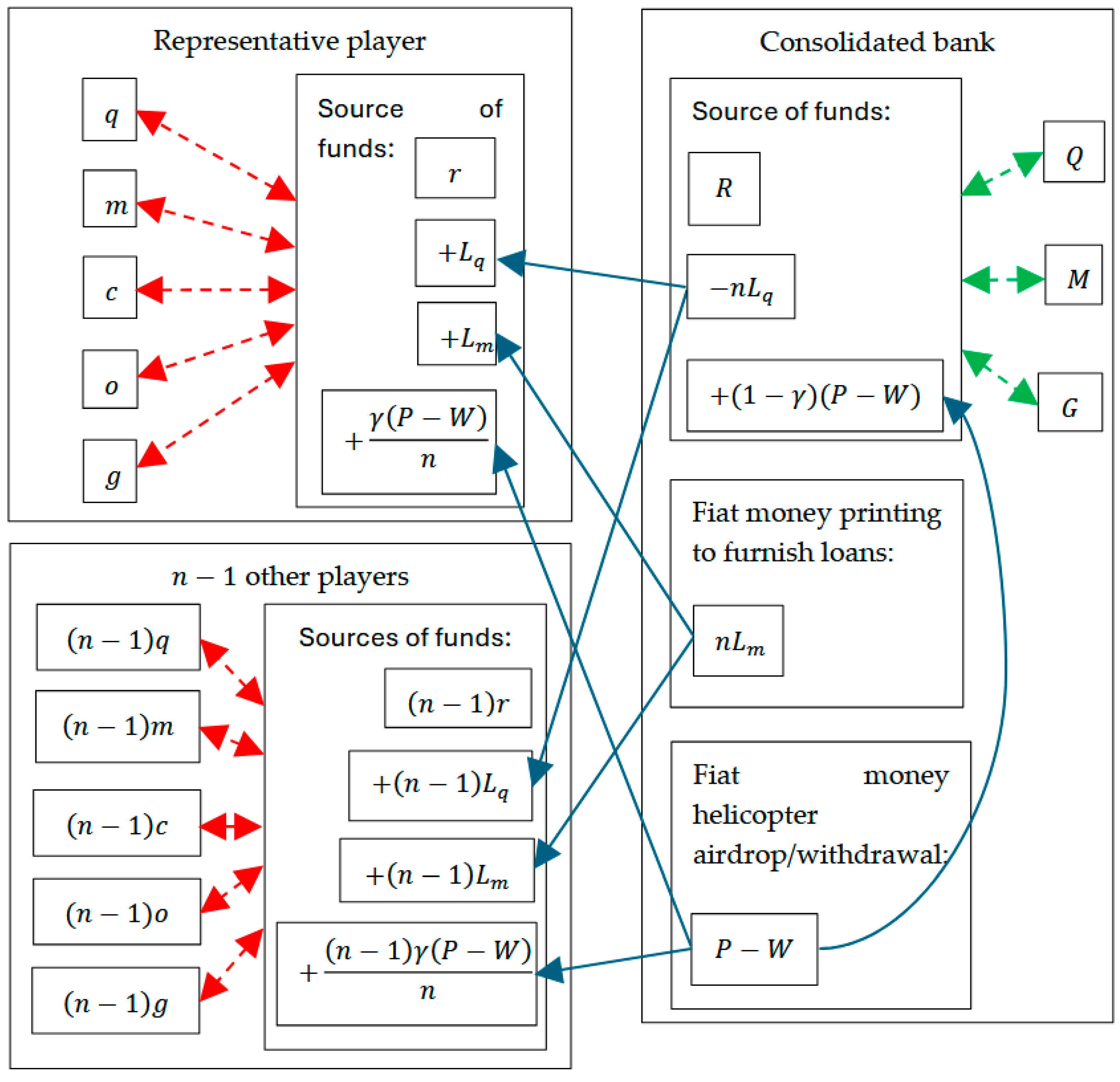
3.1. A Representative Player

A representative player  i ’s source of funds,  i = 1 , n ,   n 1 , has four components. These are resources  r 0 , a hard money loan  L q 0 , a fiat money loan  L m 0 , and a fiat money helicopter airdrop/withdrawal  γ P W n R , from the bank. Examples of player  i ’s resources  r  are income, inheritance, governmental support, and gifts. Two kinds of hard money and one kind of fiat money  m 0  are modeled. The first kind of hard money  q 0  is simply referred to as hard money, of which Bitcoin is an example as an approximation. The second kind of hard money is gold  g 0 , which is also an approximation since ca 1% new gold is mined every year (World Gold Council, 2024). Player  i ’s source of funds is allocated into hard money  q , fiat money  m , consumption  c 0 , other assets  o 0 , and gold, i.e.,
                    r + L q + L m + γ P W n = q + m + c + o + g
where the parameter  γ 0 γ 1 , defines the fraction or share of newly printed money allocated to the player in the model, or the fraction withdrawn from the player,  P 0  is money printing, and  W 0  is money withdrawal. In the player’s resource constraint (1), the left-hand side is the player’s source of funds and the right-hand side is its use of funds. All the terms in (1) are in nominal terms in some currency, e.g., USD, and not in real terms, acknowledging that inflation is accounted for separately in Section 3.3.
The player has an additive money-in-utility  u  function with seven inputs, i.e., hard money  q , fiat money  m , consumption  c , other assets  o , gold  g , a hard money loan  L q , and a fiat money loan  L m . The player earns an exogenously determined interest rate  I j t R , j = q , m , o , g , for its asset holdings from the open market. First, the player’s holding of hard money  q  is multiplied with  1 + I q I q R  to account for the hard money depositing interest rate  I q . Raising to the exponent  α q 0  gives the input  1 + I q q α q . Second, the player’s holding of fiat money  m  is multiplied with  1 + I m I m R  to account for the fiat money depositing interest rate  I m . In addition, division by  1 + π π R  occurs to account for the inflation rate  π . Raising to the exponent  α m 0  gives the input  1 + I m 1 + π m α m .
Third, the player’s consumption  c 0  is raised to the exponent  α c 0 . Consumption  c  differs from other assets  o 0  in two ways: (1) Consumption  c  pertains to the utilization of goods and services for personal satisfaction or utility, whereas other assets  o  represent durable goods or investments. (2) In contrast to other assets  o , consumption  c  does not yield interest or financial gains for the player. Instead, its primary role is to promptly fulfill the player’s necessities or desires.
Fourth and fifth, the player’s holdings of other assets  o 0  and gold  g 0  are multiplied by  1 + I o I o R  and  1 + I g I g R  to account for the interest rates  I o  and  I g . The two multiplied terms are raised to the exponents  α o 0  and  α g 0 , respectively. That gives the two inputs  1 + I o o α o  and  1 + I g g α g .
Sixth, the player’s hard money loan  L q  is multiplied by  1 + r q r q 0  to account for the hard money borrowing interest rate  r q  determined by the market and assumed exogenous in this model. The multiplied terms are raised to the exponent  α q L 0 . Since the hard money loan’s impact on the player’s utility is negative, a minus sign is applied, which gives the input  1 + r q L q α q L .
Seventh, the player’s fiat money loan  L m  is multiplied by  1 + r m r m 0  to account for the fiat money borrowing interest rate  r m  determined by the market and assumed exogenous in this model. Division by  1 + π  occurs to account for the inflation rate  π . Raising to the exponent  α m L 0  and applying the minus sign since the impact on the player is negative gives the input  1 + r m 1 + π L m α m L . The seven exponents, i.e.,  α q α m α c α o α g α q L α m L , reflect the player’s preferences for asset holdings, consumption, and borrowing. Combining the seven inputs, the player’s additive utility is
u a d d = 1 + I q q α q + 1 + I m 1 + π m α m + c α c + 1 + I o o α o + 1 + I g g α g 1 + r q L q α q L 1 + r m 1 + π L m α m L
While the utility function in (2) follows an additive and power–exponent structure, alternative specifications such as Cobb–Douglas or CES (Constant Elasticity of Substitution) functions could also be considered. Cobb–Douglas utility functions (e.g.,  u a d d = c α q β m γ ) assume a multiplicative relationship among variables, often implying a constant elasticity of substitution between different assets and consumption. It ensures that all elements contribute proportionally and prevents extreme corner solutions where all resources are allocated to one variable. CES functions allow for flexible substitution patterns, where elasticity is a key parameter. This would capture diminishing marginal returns while allowing for smoother substitution effects. A Cobb–Douglas or CES function would imply that holding money and consumption are inherently complementary, implying that consumption and money holdings must increase together to provide utility, which might not align with scenarios where money holdings serve distinct roles (e.g., precautionary savings vs. transactional usage). However, an additive structure is chosen here to ensure that each component contributes independently to the utility without requiring complementarity among assets, consumption, and money holdings. The additive approach allows greater flexibility, ensuring that increased hard money or fiat money holdings do not necessarily require increased consumption to generate higher utility. Additionally, the presence of borrowing and transaction costs means that a more rigid functional form could lead to extreme allocations (e.g., consuming all or nothing), which the additive form helps to avoid. The rationale for the additive form is that the model seeks to emphasize trade-offs rather than complementarities between money holdings and consumption. This approach simplifies interpretation while capturing diminishing marginal utility effects through the exponents. The power–exponent formulation allows for flexible curvature adjustments, ensuring that preferences can exhibit concavity, convexity, or linearity depending on the chosen exponents. While complementarities between consumption and money holdings are plausible in real-world economic behavior, the additive structure facilitates a clearer separation of effects, particularly in the presence of multiple money types and transaction costs. Thus, while Cobb–Douglas and CES forms could be explored in future work to test robustness, the additive structure is preferred here because it provides independence between different financial choices and allows clearer insights into trade-offs between consumption, money holdings, and loans.
Using hard money  q  and fiat money  m  for consumption  c , and buying other assets  o  and gold  g  involve a transaction cost  ϕ 0 . The literature models it in various ways; see Feenstra (1986); Itaya and Mino (2003); Mishra and Prasad (2024); Saygılı (2012); Schmitt-Grohé and Uribe (2004); Vázquez (1998); Wang and Hausken (2022c); Zhang (2000). This article is partly related to the existing literature and defines the transaction cost as a function of both the volume of transactions in terms of consumption  c , other assets  o , and gold  g , and in terms of money holdings  q  and  m  and interest rates  I q  and  I m , i.e.,
                  ϕ = θ c + o + g λ 1 + I q q σ q + 1 + I m m σ m
where  σ q 0  and  σ m 0  are the player’s transaction cost parameters for hard money  q  and fiat money  m , respectively. They represent the ease or convenience of using each currency in transactions. The denominator  1 + I q q σ q + 1 + I m m σ m  is additive since a multiplicative denominator unrealistically would equal zero when the player holds only one currency.
The transaction cost  ϕ  in (3) aligns with real-world payment systems by modeling transaction cost as a function of economic activity, similar to how financial institutions impose fees on various transactions. In modern payment systems, transaction costs arise from credit card processing fees, bank transfer charges, currency conversion costs, and settlement fees, all of which scale with the value and frequency of transactions. The inclusion of  c o , and  g  (consumption, other assets, and gold holdings) in the transaction cost  ϕ  reflects how different forms of economic activity contribute to total payment system costs, just as purchasing goods, investing in assets, or trading gold incurs varying levels of fees in real-world financial networks. Additionally, the inverse relationship between transaction costs and liquidity preferences in the model mirrors real-world behavior, where higher costs lead economic agents to optimize payment methods, such as choosing lower-fee options or reducing transaction frequency. The discussion after Equation (3) further supports this analogy by showing how money allocation decisions are shaped by transaction costs, much like businesses and individuals deciding between cash, electronic payments, or cryptocurrencies based on cost efficiency. Thus, the model effectively captures key trade-offs in modern payment systems, particularly the balance between cost, liquidity, and transaction volume.
The parameter  λ 0  is the player’s scaling exponent for consumption  c  and buying other assets  o  and gold  g . The parameter  θ > 0  is the player’s proportional scaling parameter for the transaction cost  ϕ . The denominator in (3) sums up the amounts of hard and fiat money for transactions, raised to their respective transaction cost parameters  σ q  and  σ m . The numerator in (3) represents the value  c + o + g  of the transactions, which is raised to the scaling exponent  λ .
Subtracting the player’s transaction cost  ϕ  in (3) from the player’s utility  u a d d  in (2), and using the player’s resource constraint in (1) to rewrite the player’s gold holding as  g = r q m c o + L q + L m + γ P W n  gives the player’s utility
                u = 1 + I q q α q + 1 + I m 1 + π m α m + c α c + 1 + I o o α o + 1 + I g r q m c o + L q + L m + γ P W n α g 1 + r q L q α q L                                   1 + r m 1 + π L m α m L θ r q m + L q + L m + γ P W n λ 1 + I q q σ q + 1 + I m m σ m
In (4), the exponent  α j 0  for  j ,   j = c ,   q ,   m ,   o ,   g , L q ,   L m ,  for the first seven terms, is positive. More precisely, if  α j = 0 0 < α j < 1 α j = 1 α j > 1 , each term equals 1 and increases concavely, linearly, and convexly, respectively. Convex increase  α j > 1  sometimes causes a player to allocate all its funds into one asset, but not in (4), since three terms are subtracted, and the player strikes an allocation balance according to its resource constraint in (1). A concave increase of  α j 0 < α j < 1 , for the first five terms in (4) may be common since it expresses that the player prefers some initial allocation to each term, but with diminishing return on investment to prevent excessive allocation to any one term.
The player’s resource constraint in (1) involves six free-choice variables for the player. These are holding of hard money  q , fiat money  m , consumption  c , other assets  o , hard money loan  L q , and fiat money loan  L m , where gold  g = r q m c o + L q + L m + γ P W n  is implicitly determined by (1).

3.2. The Bank

The bank’s source of funds has three components. These are the bank’s resources  R 0 , the bank’s provision of hard money loans  n L q  to the  n  players, which has a negative impact, and a fiat money helicopter airdrop/withdrawal  1 γ P W R , which are deployed into hard money  Q 0 , fiat money  M 0 , and gold  G 0 , i.e.,
                    R n L q + 1 γ P W = Q + M + G
where  1 γ  denotes the fraction of the helicopter airdrop/withdrawal assigned to the bank, and  n  is the number of players that borrow hard and fiat money from the bank. The bank does not hold other assets. Assume that the bank prints fiat money to provide fiat money loan  n L m  to the players. In the bank’s resource constraint (5), the left-hand side is the bank’s source of funds and the right-hand side is its use of funds. The bank’s fiat money loan  n L m  to the  n  players is abbreviated in (5) since it shows up on both the right-hand side and the left-hand side.
Figure 1 shows the flows of funds between the bank and the players, distinguishing between the representative player and the  n 1  other players. The flows of funds are shown with blue one-way solid arrows, i.e., hard money loans  n L q  from the bank’s source of funds, fiat money loans  n L m  printed by the bank, and fiat money helicopter airdrop/withdrawal, which the bank also allocates/withdraws to/from its own source of funds. The five red dashed two-way arrows show how the representative player allocates its source of funds (the left-hand side of (1)) into its assets  q ,   m ,   c ,   o ,   g  (the right-hand side of (1)), choosing its six variables  q ,   m ,   c ,   o ,   L q , and  L m . The setup is analogous for the  n 1  other players. The three green dashed two-way arrows show how the bank allocates its source of funds (the left-hand side of (5)) into its assets  Q ,   M ,  and  G  (the right-hand side of (5)), choosing its three variables  Q ,   M , and  P - W .
Typically, a central bank determines the fiat money supply, and commercial banks provide loans in an economy. The Cantillon effect indicates that changes in the fiat money supply cause uneven wealth distribution, favoring early recipients of new money over others (Bordo, 1983). For simplicity, to prevent too many players, assume that the bank consolidates the roles of a commercial bank and a central bank. For this article’s purposes, the bank’s utility function incorporates features of both commercial and central banks. The consolidated bank determines the supply of fiat money. That is, the bank can print  P P 0 , fiat money at negligible cost, or withdraw  W W 0  fiat money. Examples that consider the bank and central banks as a unified entity are Chen et al. (2017); Gertler and Kiyotaki (2015); Wang and Hausken (2021b). Examples that assume a consolidated central bank government entity are McCallum (1997) and Masciandaro and Volpicella (2016). The fiat money printing and withdrawal impact the inflation rate  π π R . The bank cannot print or withdraw hard money  Q  since the supply of hard money is determined exogenously. The bank is assumed to offer hard money loans  n L q  and fiat money loans  n L m  to the players.
The bank has an additive utility function with five inputs. First, hard money  Q  is multiplied with  1 + I q  to account for the hard money depositing interest rate  I q  in the open market. Thereafter, the multiplied terms are raised to the exponent  β Q 0 . That gives the input  1 + I q Q β Q .
Second, fiat money  M  is multiplied with  1 + I m  to account for the fiat money depositing interest rate  I m  in the open market. Thereafter, division with  1 + π  occurs to account for the inflation rate  π . Raising to the exponent  β M 0  gives the input  1 + I m 1 + π M β M . Here,  M  is the bank’s holding of fiat money after printing and lending fiat money  n L m  to the  n  players, printing an amount  P  of fiat money, and withdrawing an amount  W  of fiat money, which causes a fiat money helicopter airdrop/withdrawal of  1 γ P W  to the bank.
Third, the bank’s gold holding  G  is multiplied with  1 + I g  to account for the interest rate  I g . Raising to the exponent  β G 0  gives the input  1 + I g g β G .
Fourth and fifth, assume that the bank retains the utility of the hard money loan  n L q  and the fiat money loan  n L m  it lends to the players. The term  n L q  is multiplied with  1 + r q  to account for the hard money borrowing interest rate  r q . The term  n L m  is multiplied with  1 + r m  to account for the fiat money borrowing interest rate  r m  and divided by  1 + π  to account for the inflation rate  π . The two loans are raised to the exponents  β q L 0  and  β m L 0 , respectively. Multiplication by the number of players  n  gives the inputs  n 1 + r q L q β Q L  and  n 1 + r m 1 + π L m β M L . The five exponents, i.e.,  β Q β M β G β Q L β M L , reflect the bank’s preferences for asset holdings and lending. Combining the five inputs, and using the bank’s resource constraint in (5) to rewrite the bank’s gold holding as  G = R n L q + 1 γ P W Q M , the bank’s utility is
U = 1 + I q Q β Q + 1 + I m 1 + π M β M                   + 1 + I g R n L q + 1 γ P W Q M β G                   + n 1 + r q L q β Q L + n 1 + r m 1 + π L m β M L
The bank cannot lend out more hard money than it holds, i.e.,  n L q Q . In (6), the exponent  β j 0  for asset  j ,   j = Q ,   M , L q , L m  is positive. More precisely, if  β j = 0 0 < β j < 1 α j = 1 β j > 1 , each term equals 1 and increases concavely, linearly, and convexly, respectively.
The bank’s resource constraint in (5) involves three free-choice variables for the bank. These are holding of hard money  Q , fiat money  M , and money printing  P  minus withdrawal  W , i.e.,  P W , where gold  G = R n L q + 1 γ P W Q M  is implicitly determined by (5). The player and the bank choose their strategies simultaneously and independently in a one-period game.

3.3. The Inflation Rate  π

The inflation rate  π  is defined as
                    π = n L m + P W n q + Q + n m + M
where  q  and  m  are the hard and fiat money held by the representative player. The parameters  P  and  W  are the amounts of fiat money printed and withdrawn by the bank. Therefore, the term  n q + Q + n m + M  in the denominator in (7) represents the combined amount of hard and fiat money in circulation. The parameter  n  is the number of players that borrow hard and fiat money from the bank. The parameter  L m  is the amount of fiat money that each player borrows. The bank prints fiat money  n L m  to lend to the  n  players. Thus,  n L m + P W  in the numerator in (7) expresses how much new fiat money is printed by the bank.
Equation (7) defines inflation as a function of fiat money printing, withdrawal, and borrowing, relative to the total hard and fiat money in circulation. This formulation shares conceptual similarities with the Quantity Theory of Money (Fisher, 1911), which states that the product of the money supply and the money velocity equals the nominal gross domestic product, which equals the product of the average price level and the number of transactions over the given time period. However, the current model does not explicitly incorporate velocity, assuming instead that inflation is primarily driven by changes in the fiat money supply through banking actions. This simplification aligns with monetary models that emphasize the supply-side determinants of inflation but do not account for the dynamic role of money velocity, which can fluctuate due to liquidity preferences, financial innovations, or macroeconomic conditions. Furthermore, expectations about future inflation, a key component in New Keynesian models, are not modeled explicitly. While price-level expectations can influence borrowing, lending, and money-holding behavior, this model assumes a static environment where inflation results directly from money supply changes. Future research may explore extensions incorporating adaptive or rational expectations to refine the inflationary dynamics within the hard and fiat money coexistence framework.

4. Analyzing the Model

This article jointly solves the player’s and the bank’s first-order conditions, which amounts to determining their best responses to each other in the one-period game. The first-order conditions are not analytically solvable and are illustrated numerically. The numerical illustration is tested for robustness to changes in parameter values. Determining mutually best responses, which is a necessary condition for Nash equilibrium, is convenient for the analysis and resembles determining the Nash equilibrium where no player prefers to deviate unilaterally. The resemblance is high for games over one period, with complete information, where multiple equilibria are not expected, where mixed strategies are not analyzed, and where no apparent need exists to eliminate dominated strategies iteratively (e.g., as in the prisoner’s dilemma where both (Cooperate, Cooperate) and (Defect, Defect) can be considered mutually best responses, depending on the stage of reasoning).

4.1. The Player’s Six Interior First-Order Conditions

Inserting (7) into (4), differentiating (4) with respect to the player’s six strategic free-choice variables  q ,   m ,   c ,   o ,   L q , and  L m  and setting each expression to zero, give the player’s six first-order conditions shown in (A1) in Appendix B.

4.2. The Bank’s Three Interior First-Order Conditions

Inserting (7) into (6), differentiating (6) with respect to the bank’s three strategic free-choice variables  Q M , and  P W , and setting each expression to zero, the bank’s three first-order conditions are shown in (A2) in Appendix C.

5. Illustrating and Interpreting the Model

5.1. Benchmark Parameter Values and Model Setup

To illustrate the solution in Section 4, this section alters the 26 parameter values relative to the following plausible benchmark parameter values:  n = 1 I q = I m = I o = I g = 2 % r q = r m = 5 % α q = α m = α c = α o = α g = α q L = α m L = 9 10 β Q = β M = β G = β Q L = β M L = 9 10 σ q = 1 σ m = 1.2 γ = 0.55 λ = 1.5 θ = 1 r = 1000 ,   R = 41,485.53 . The units of the assets and loans can be USD. The utilities are determined by (4) and (6). The other variables and parameters are dimensionless. The analysis is made using the Mathematica 14.1 software package (www.wolfram.com/mathematica/?source=nav) accessed on 2 March 2025. The code is available on request.

5.2. Economic Assumptions and Justifications

First,  n = 1  expresses only one representative player. Second,  I q = I m = I o = I g = 2 %  expresses the equal depositing interest rate for hard and fiat money, other assets, and gold in the open market. Third,  r q = r m = 5 %  expresses the equal borrowing interest rate for hard and fiat money. The borrowing interest is higher than the assets depositing interest rate. Fourth,  α q = α m = α c = α o = α g = α q L = α m L = 9 10  expresses that the player’s first seven terms in (4) increase with slight concavity. The realism of this assumption is discussed after (4). Similarly,  β Q = β M = β G = β Q L = β M L = 9 10  expresses slight concavity for the five terms for the bank’s utility in (6), with similar justification. Fifth,  σ q = 1  reflects a higher transaction cost for hard money than that for fiat money where  σ m = 1.2 . Sixth,  γ = 0.55  reflects that the player receives 22% more than the bank receives from the bank’s fiat money helicopter airdrop/withdrawal. Seventh,  λ = 1.5 > σ m > σ q  is chosen to ensure that the player is willing to consume or buy other assets  o  and gold  g . Eighth, the choice of  θ = 1  is driven by simplicity and the fact that the value 1 appears reasonable when no other value appears to be more convincing. Ninth, the choices  r = 1000  and  R = 41,485.53  are made to ensure specifically that the inflation rate  π = 2 %  and  P W = 0 .

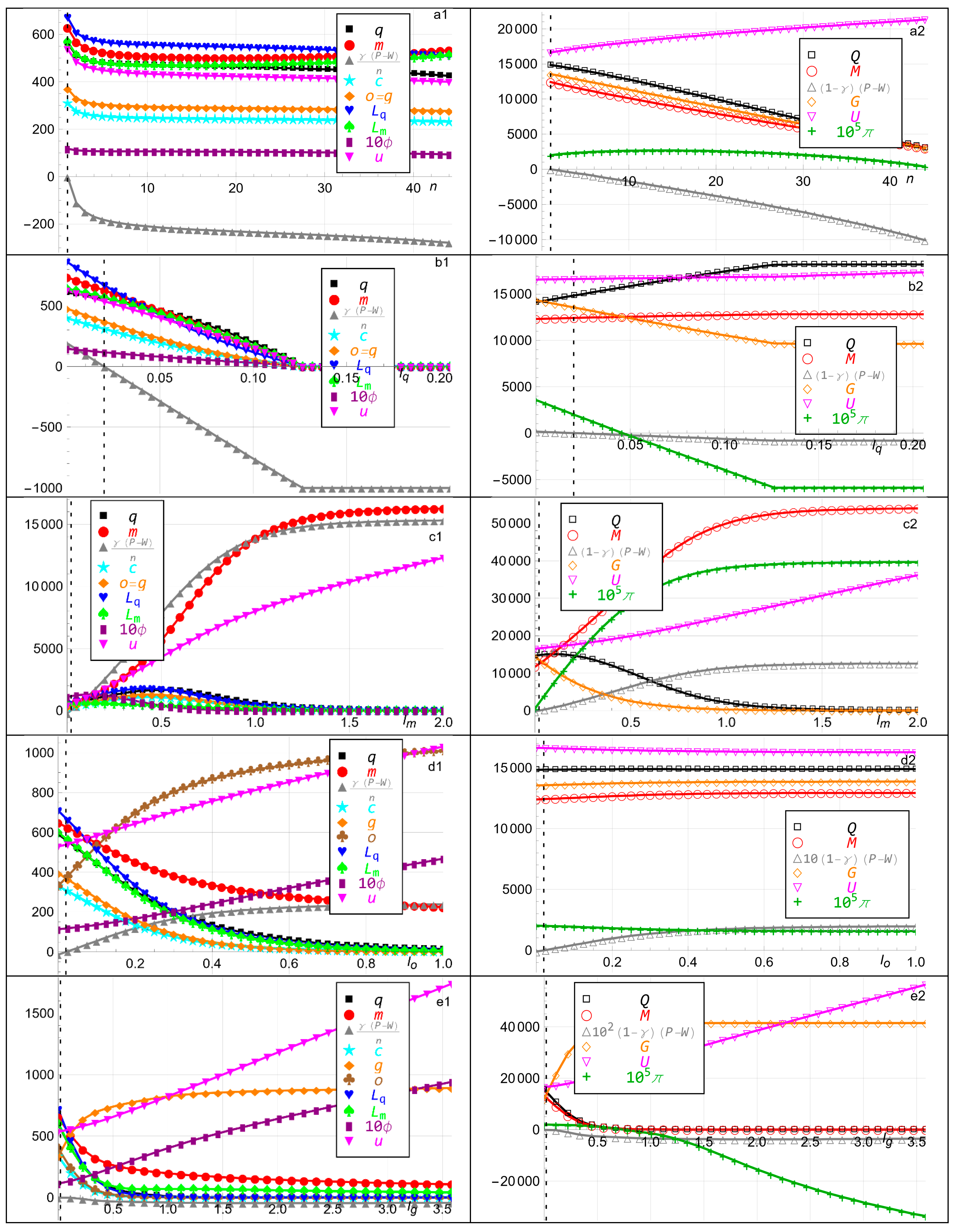
5.3. Interpretation of Figure 2 and Approach to Parameter Variations

With these benchmark parameter values, the benchmark solution is  q = 562.69 m = 628.21 c = 309.57 o = g = 369.97 L q = 671.4 L m = 569 u = 538.07 Q = 14,841.02 M = 12,418.3 G = 13,554.81 P W = 0 , and  U = 16,623.94 . At the benchmark, the inflation rate  π = 2 % , i.e., the common inflation rate target is 2% in many fiat economies. The player’s transaction cost  ϕ = 11.69 , i.e.,  1.11 %  of the sum of consumption  c , other assets  o , and gold  g , and 3.77% of the consumption  c . The first percentage approximates the lowest average credit card processing fee. The second percentage slightly exceeds the highest average credit card processing fee. The average cost of credit card processing fees falls within the range of 1.5% to 3.5% (Forbes Advisor, 2024).
Figure 2. The player’s hard money  q , fiat money  m , helicopter airdrop/withdrawal  γ P W n , consumption  c , other assets  o , gold  g , hard money loan  L q , fiat money loan  L m , transaction cost  ϕ  and utility  u , the bank’s hard money  Q , fiat money  M , the bank’s fiat money helicopter airdrop/withdrawal  1 γ P W , gold  G , utility  U , and the inflation rate  π , respectively, relative to the benchmark parameter values  r = 1000 ,   R = 41,485.53 n = 1 I q = I m = I o = I g = 2 % r q = r m = 5 % α q = α m = α c = α o = α g = α q L = α m L = 9 / 10 β Q = β M = β G = β Q L = β M L = 9 / 10 σ q = 1 σ m = 1.2 γ = 0.55 λ = 1.5 θ = 1 . The multiplication of  π  by 105 and 107 and the multiplication of  ϕ  and  ( 1 γ ) ( P W )  by 10 and 100 are for scaling purposes.
Economies 13 00080 g002aEconomies 13 00080 g002bEconomies 13 00080 g002cEconomies 13 00080 g002dEconomies 13 00080 g002eEconomies 13 00080 g002f
Figure 2 illustrates the player’s and the bank’s variables in response to variations in the 26 parameter values, relative to the plausible benchmark parameter values. The x-axis in each panel represents the labeled parameter. The y-axis represents the player’s and the bank’s variables, distinguishing between the fiat money helicopter airdrop/withdrawal  γ P W n  to/from the player and the fiat money helicopter airdrop/withdrawal  1 γ P W  to/from the bank. In Figure 2, each of the 26 parameter values is altered from its benchmark marked with a vertical dashed line in each panel, while the other 25 parameter values are kept at their benchmarks. The multiplication of  π  by  10 5  and  10 7  and the multiplication of  ϕ  and  1 γ P W  by 10 and 100 are for scaling purposes. The six most interesting panels are interpreted in this section. The remaining 20 panels are interpreted in Appendix D.

5.4. Effects of Hard and Fiat Money Interest Rates on Inflation and Utility

In Figure 2b, as the interest rate  I q  of hard money increases through the benchmark  I q = 2 % , the bank adjusts its resource allocation by intuitively increasing its hard money holding  Q , decreasing its gold holding  G , and slightly increasing its fiat money holding  M . The bank withdraws fiat money, causing a decrease in the inflation rate  π , and slightly increasing utility  U . The bank faces limitations. It cannot infinitely increase its hard money holdings  Q , decrease its gold holdings  G , and withdraw fiat money. As  I q  increases beyond  I q = 4.61 % , the inflation rate  π  becomes negative. A negative inflation rate expresses deflation, reflecting reduced fiat money in circulation. After  I q  reaches 12.65%, when the inflation rate is  π = 5.88 % , the bank’s holdings of hard money  Q , fiat money  M , and gold  G  remain relatively constant, and all the player’s variables except  γ P W / n  reach zero. That expresses a bankrupt player where both sides of the player’s resource constraints in (1) equal zero. That explains the kinks in the curves. The bank’s money withdrawal expressed with the negative  γ P W  detrimentally decreases all the player’s variables, which may sound counterintuitive since higher  I q  may be expected to be positive. A paradoxical result is that a higher hard money interest rate  I q , instead of benefiting the player, reduces utility and leads to bankruptcy. This happens because the bank withdraws fiat money, causing deflation and liquidity shortages, which severely constrain player allocation. While the bank benefits initially, it cannot expand its hard money holdings indefinitely, highlighting the trade-off between curbing inflation and destabilizing the financial system through excessive monetary tightening.
In Figure 2c, as the interest rate  I m  of fiat money increases moderately above the benchmark  I m = 2 % , which benefits both the player and the bank in terms of higher utilities  U  and  u , the player’s variables, and especially its hard money loan  q , are inverse U-shaped, but eventually approach zero as allocation to fiat money holdings  M  and  m  become the main focus for the player and the bank. The bank’s and the player’s  M  and  m  increase logistically and level out when no further funds are available. Then, no funds are allocated elsewhere. The bank prints fiat money  P W  to some extent to benefit from the higher  I m , accepting the increased inflation rate  π . Conversely, when  I m  decreases below the benchmark  I m = 2 % , all the player’s variables decrease, while all the bank’s variables decrease except gold  G . A counterintuitive result is that while a moderate increase in the fiat money interest rate  I m  benefits both the player and the bank initially, it eventually eliminates hard money from circulation. As  I m  rises, the player shifts entirely to fiat money holdings, abandoning hard money loans and assets. The bank facilitates this shift by printing more fiat money, increasing inflation but profiting from higher interest returns. However, when  I m  falls below the benchmark, both the player and the bank suffer, with declining utility and reduced financial activity. This highlights the fragility of monetary balance, where a strong fiat money preference can crowd out hard money entirely.

5.5. Impact of the Number of Players on Inflation and Bank Lending

In Figure 2a, as the number  n  of players increases above the benchmark  n = 1 , more players take up loans  n L q  and  n L m . That decreases the bank’s hard money holding  Q . The inflation rate  π  is inverse U-shaped with a maximum  π = 2.67% when  n = 14 . To constrain and eventually decrease the inflation rate  π , since more players incur fiat money loans  n L m , the bank withdraws fiat money shown with the decreasing  1 γ P W , which goes negative. Inverse U shape means that the variable increases as the parameter increases, but declines after a certain point. That decreases the bank’s source of funds on the left-hand side of (5), which decreases the bank’s holdings of hard money  Q , fiat money  M , and gold  G . The bank’s utility increases due to its lending, as the two last terms in (6) increase. The bank’s fiat money withdrawal  P W  negatively impacts the player’s source of funds on the left-hand side of (1). That causes the player’s holdings of hard money  q , gold  g , other assets  o , and consumption  c  to decrease. The eventually decreasing inflation rate  π  causes the player to increase its fiat money holding  m , and even to increase its fiat money loan  L m . Conversely, the player decreases its hard money loan  L q , i.e., borrows less hard money as the number  n  of players increases. A counterintuitive result is that while more players taking loans might be expected to drive inflation continuously higher, the bank’s fiat money withdrawal eventually reverses this trend, first increasing inflation and then reducing it. This happens because, although additional borrowers create higher demand for fiat money, the bank counteracts this by tightening liquidity. Another key insight is that while the bank profits from increased lending, players face tighter financial conditions, shifting toward fiat money while reducing hard money and asset holdings. This dynamic highlights the bank’s dual role, balancing lending profits with inflation control through fiat money withdrawals.

5.6. The Impact of Fiat Money Allocation on Inflation and Utility

In Figure 2s, as the fraction  γ  of fiat money helicopter airdrop/withdrawal allocated to the player increases through the benchmark  γ = 0.55 , the bank prints more fiat money  P W . That causes all the player’s variables to be U-shaped except the transaction cost, which equals  ϕ = 54.47  when  γ = 0 . The player’s fiat money holding  m  and fiat money loan  L m  are additionally inverse U-shaped as  γ  approaches 1. That occurs because the player no longer needs to borrow fiat money  L m , and because inflation discourages holding fiat money  m . The bank’s fiat money printing  P W  becomes overwhelming, causing  m =   L m = 0  when  γ = 1 . The money printing  1 γ P W  allocated to the bank and the bank’s hard money holding  Q  are inverse U-shaped. Its utility  U  is slightly inverse U-shaped. The inflation rate  π  increases exponentially consistently with (7). That causes the bank to decrease its fiat money holding  M . Its gold holding is U-shaped and decreases sharply towards  lim γ 1 G = 0 . The player particularly increases its hard money holding  q  and hard money loan  L q , and earns higher utility  u . That shows that a high inflation rate  π  may benefit the player if hard money  q  is available, in addition to fiat money  m . The bank’s hard money holding  Q  is inverse U-shaped and its gold holding  G  is U-shaped. As  γ  decreases below the benchmark  γ = 0.55 , the player holds more fiat money  m  because of the negative inflation rate  π < 0 , and incurs a higher fiat money loan  L m  because of the bank’s substantial money withdrawal expressed with a negative  P W . A counterintuitive result is that as the player receives a larger fraction  γ  of fiat money printing, inflation rises sharply, yet the player benefits from holding more hard money rather than fiat money. This happens because extreme inflation discourages fiat money holdings and borrowing, pushing the player toward hard money. Meanwhile, the bank’s utility follows an inverse U shape, as excessive fiat money printing forces the bank to reduce its fiat holdings and liquidate gold reserves to stabilize its balance sheet. This highlights a key insight: high inflation can favor players if hard money remains an option, while the bank faces constraints in managing liquidity.

5.7. The Role of Transaction Costs in Money Allocation and Inflation

In Figure 2p, as the player’s transaction cost parameter  σ q  for hard money  q  increases through the benchmark  σ q = 1 , the transaction cost  ϕ  of using hard money  q  intuitively decreases as  σ q  appears in the denominator of the transaction cost function  ϕ  in (3). Consequently, the player’s transaction cost  ϕ  decreases logistically,  lim σ q ϕ = 0 . That initially causes the player’s hard money holding  q  to increase and reach a maximum when  σ q = 1.2 = σ m . Thereafter,  q  and the player’s fiat money holding  m  decrease logistically towards constants, while the player’s consumption  c  and holdings of other assets  o , gold  g , and utility  u  increase logistically towards constants consistently with the transaction cost approaching  lim σ q ϕ = 0 . The bank’s increasing fiat money printing  P W  induces the player to borrow less hard money  L q  and borrow less fiat money  L m , causing the bank to marginally increase its holdings of hard money  Q , fiat money  M , and gold  G , and earn marginally lower utility  U . The inflation rate  π  is slightly U-shaped, reaching a minimum of  1.98 %  at  σ q = 1.2 = σ m . As  σ q  decreases below  σ q = 1 , the player substantially allocates to fiat money  m  according to (3) to limit the transaction cost  ϕ . A surprising result is that as the hard money transaction cost parameter  σ q  increases, the player’s actual cost of using hard money decreases, leading to a temporary rise in hard money holdings. However, beyond a threshold, the player shifts away from hard money, reallocating to fiat money and other assets. The bank reacts by printing more fiat money, which induces the player to borrow less overall, causing the bank to experience lower utility, as reduced borrowing limits its lending profits. Inflation follows a U-shaped pattern, initially declining but rising again as transaction costs shift player behavior. This highlights how transaction costs can determine the coexistence of hard and fiat money, rather than interest rates alone.

5.8. Bank Preferences and Strategic Fiat Money Printing

In Figure 2w, as the bank’s exponent for fiat money  β M  increases above the benchmark  β M = 9 / 10 , the bank naturally increases its fiat money holding  M , and decreases its holdings of hard money  Q  and gold  G . The bank prints fiat money moderately, causing a noticeable rise in the inflation rate  π . Notably, despite the increased inflation rate  π , the bank continues to increase its fiat money holding  M . This is due to the overriding impact of the increased  β M  compared to the impact of the heightened inflation rate  π . The bank’s utility  U  increases with  β M . The player’s holding of fiat money  m  and fiat money loan  L m  are inverse U-shaped. The player obtains fiat money helicopter airdrop  γ P W  from the bank. The player increases its holdings of hard money  q , other assets  o , gold  g , and hard money loan  L q  concavely toward their limits. Overall, the player’s utility  u  increases. Thus, both the player and the bank benefit from a higher  β M . Conversely, when  β M  decreases above the benchmark  β Q = 9 / 10 , all the player’s variables decrease. All the bank’s variables decrease except  G . A key insight is that as the bank’s preference for fiat money ( β M ) increases, it prioritizes fiat holdings over hard money and gold, despite rising inflation. The bank benefits more from fiat money than it loses from inflation, while the player initially gains but later reduces fiat borrowing, creating an inverse U-shaped effect. Furthermore, higher  β M  initially benefits both the bank and the player by increasing fiat money availability. However, excessive reliance on fiat money eventually reduces player borrowing and disrupts balance. Conversely, a decline in  β M  leads to economic contraction, highlighting the importance of fiat money dominance for stability.

5.9. Table Illustration

Table 1 summarizes the player’s variables, the bank’s variables, and the inflation rate  π  for the 26 panels in Figure 2.

6. The Role of Prices in the Model

The prices in the model are indirectly determined by the interaction of several parameters and variables related to both the representative player’s and the bank’s strategies, including the utility derived from holdings, loans, and transaction costs for hard and fiat money. The price determinants are as follows:
  • Interest Rates: Higher hard money interest rates lead to increased holdings by the bank and decreased inflation, but paradoxically reduce the utility for the player by constraining its allocation towards hard money. Conversely, higher fiat money interest rates encourage money printing, increase inflation, and eventually diminish the coexistence of hard money, benefiting both the player and the bank in terms of utility.
  • Utility Exponents: The utility exponents for both hard and fiat money for the player and the bank (their preferences for holding different types of money) determine how resources are allocated between these two forms of money. For instance, higher exponents for fiat money holding by the bank increase its allocation towards fiat money, impacting inflation rates.
  • Transaction Costs: Transaction costs associated with using hard or fiat money significantly impact the player’s allocation preferences. Lower transaction costs for one form of money increase its attractiveness and holding levels, indirectly influencing market prices.
  • Fiat Money Supply: The bank’s ability to print or withdraw fiat money directly influences inflation, which in turn affects the nominal values of goods, assets, and money in the economy. More fiat money printing generally increases inflation and nominal prices, whereas withdrawal reduces inflation.
  • Inflation Rate: The inflation rate in (7) is a key determinant of the price level and is influenced by the amount of fiat money in circulation relative to hard money and the volume of loans.
  • Player’s Strategic Allocation: The representative player allocates its resources across consumption, holdings (hard and fiat money, gold, and other assets), and loans. Changes in the player’s resource allocation impact its transaction costs and overall utility, indirectly determining the price it is willing to pay for goods and loans.
  • Bank’s Strategic Behavior: The bank adjusts its holdings and lending strategies based on market conditions, fiat money availability, and inflation. Its actions, such as increasing fiat money lending or withdrawing funds, directly impact the prices by modifying the monetary base.
  • Key Insights: Inflation and the relative utility derived from different forms of money play central roles in price determination. The strategic interactions between the representative player and the bank create mutually best response conditions where prices stabilize depending on the chosen parameter values.

7. Interpreting the Model

The authors have identified 12 insights of the model.

7.1. Most Essential Insights

  • Increasing the hard money interest rate causes fiat money withdrawal and, paradoxically, lowers player utility and, eventually, bankruptcy by restraining the player’s allocation possibilities. The inflation decreases and eventually transitions to deflation. The bank’s allocation possibilities are also restrained, but it receives higher utility through increasing its hard money holding and decreasing its gold holding. Thus, a higher interest rate for hard money does not necessarily make it more attractive for the player but, rather, may benefit the bank at the player’s expense, as shown in Figure 2b.
  • In contrast, increasing the fiat money interest rate causes fiat money printing, inflation, and higher utilities for the player and bank. The player first increases and thereafter decreases all its variables except its fiat money holding and utility. That causes hard and fiat money not to coexist. This highlights how fiat money policies can fundamentally alter the financial system, potentially making hard money obsolete, as shown in Figure 2c.
  • More players mean more fiat money loans, which benefits the bank. That encourages the bank to withdraw fiat money and decrease its holdings of hard and fiat money and gold. The bank’s fiat money withdrawal causes lower utility for each player. As the inflation eventually decreases, each player increases its fiat money holding and fiat money borrowing and holds less hard money. This is crucial for central banks, as it suggests that an increasing number of borrowers does not necessarily benefit the broader economy, as shown in Figure 2a.
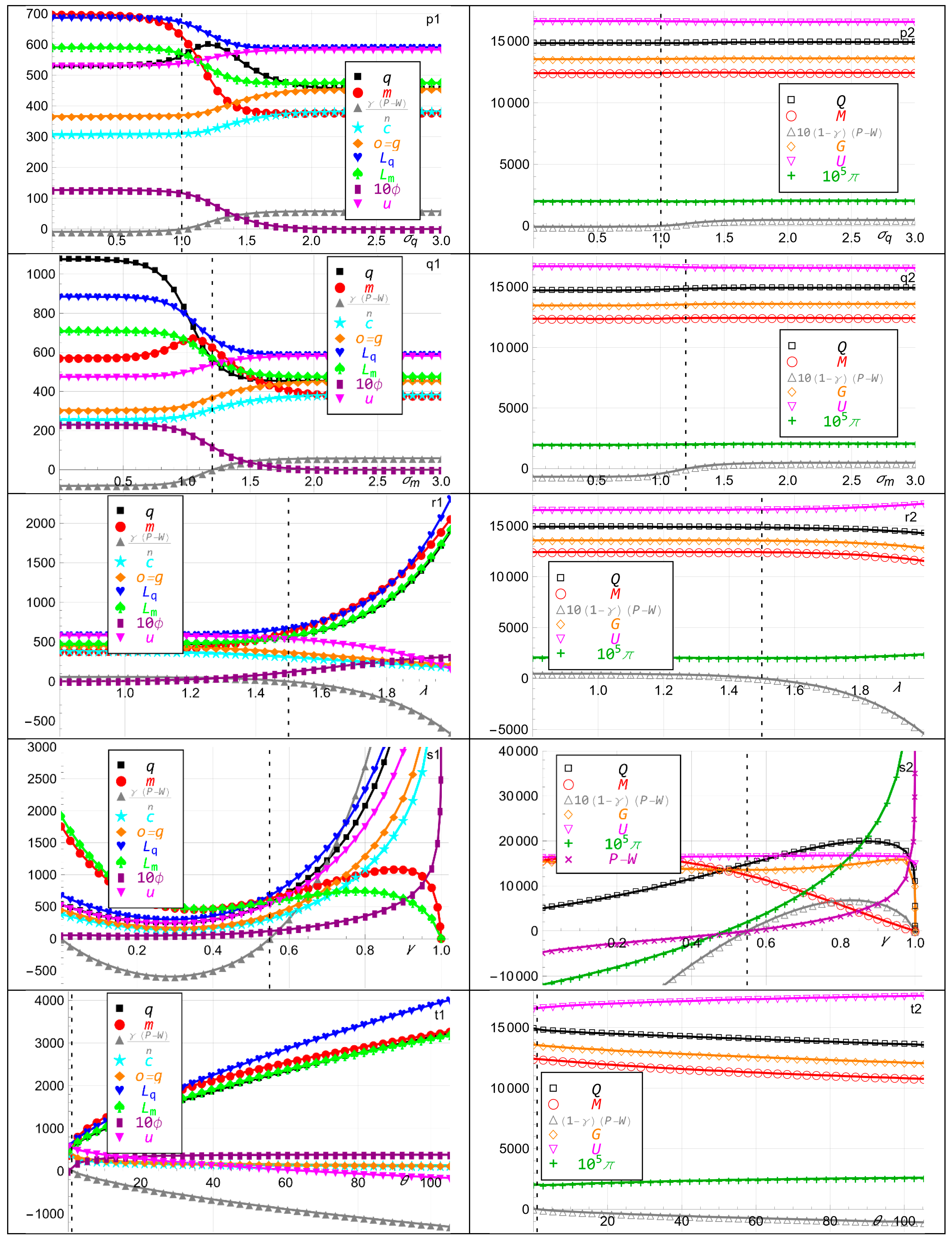
  • Allocating more printed fiat money to the player causes inflation and induces the player to consume more, hold more hard money, borrow more hard money, and, eventually, hold less fiat money and borrow less fiat money. The inflation benefits the player since hard money is available in addition to fiat money. The bank is relatively unaffected. It benefits from the player’s increased borrowing but suffers from the increased allocation to the player. Allocating less printed fiat money to the player causes deflation. These results suggest that central banks should carefully monitor the impact of money printing to avoid destabilizing inflation, as shown in Figure 2s.
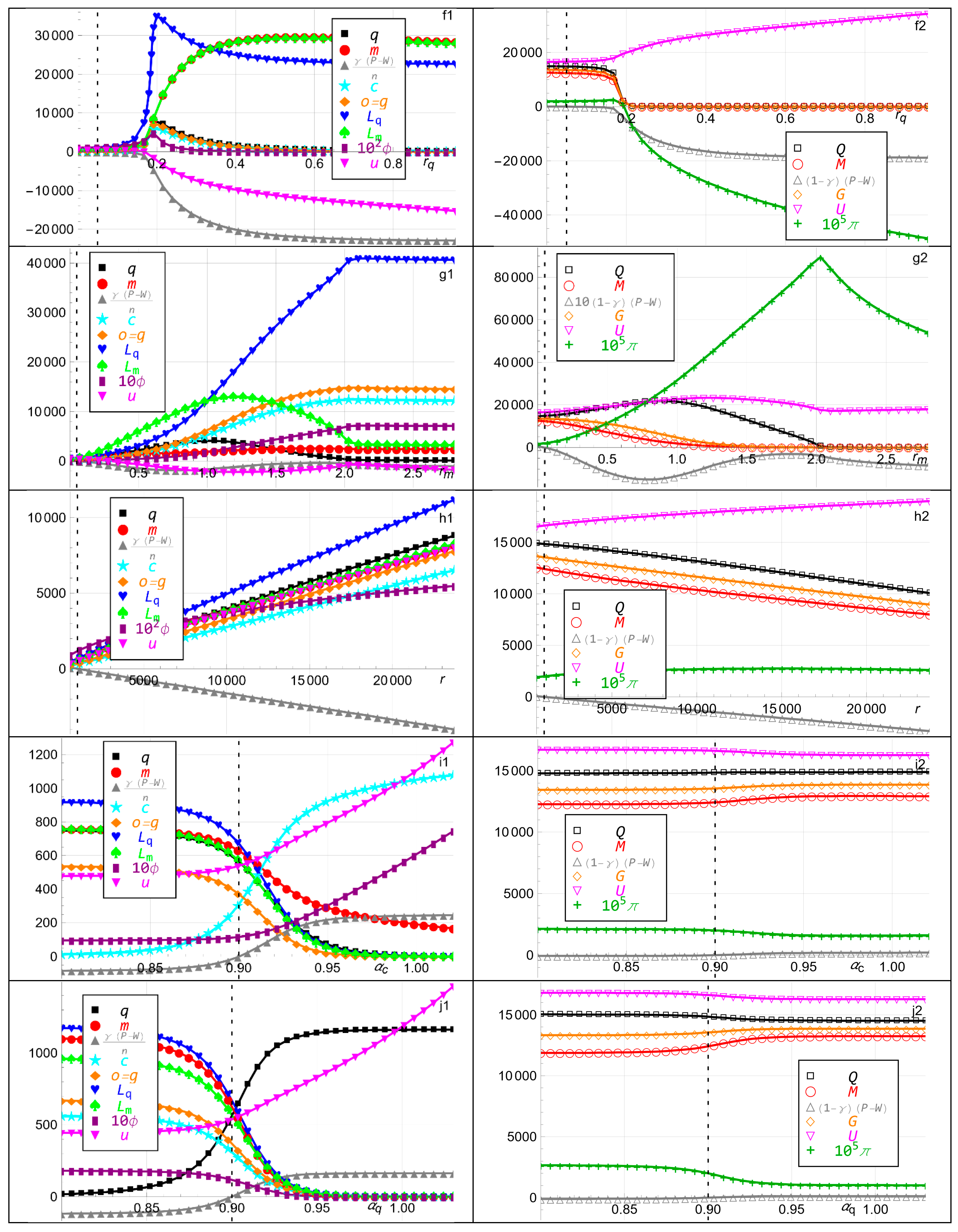
  • Increasing the player’s hard money transaction cost parameter, and analogously for the fiat money transaction cost parameter, causes the player to consume more, hold more gold, hold less fiat money, borrow less, and earn higher utility. Hence, hard and fiat money can coexist with different transaction costs. The bank is relatively unaffected but prints fiat money and earns lower utility, which causes the player to first increase and then decrease its hard money holding. This shows that transaction costs play a critical role in determining which form of money dominates, not just inflation or interest rates, as shown in Figure 2p.
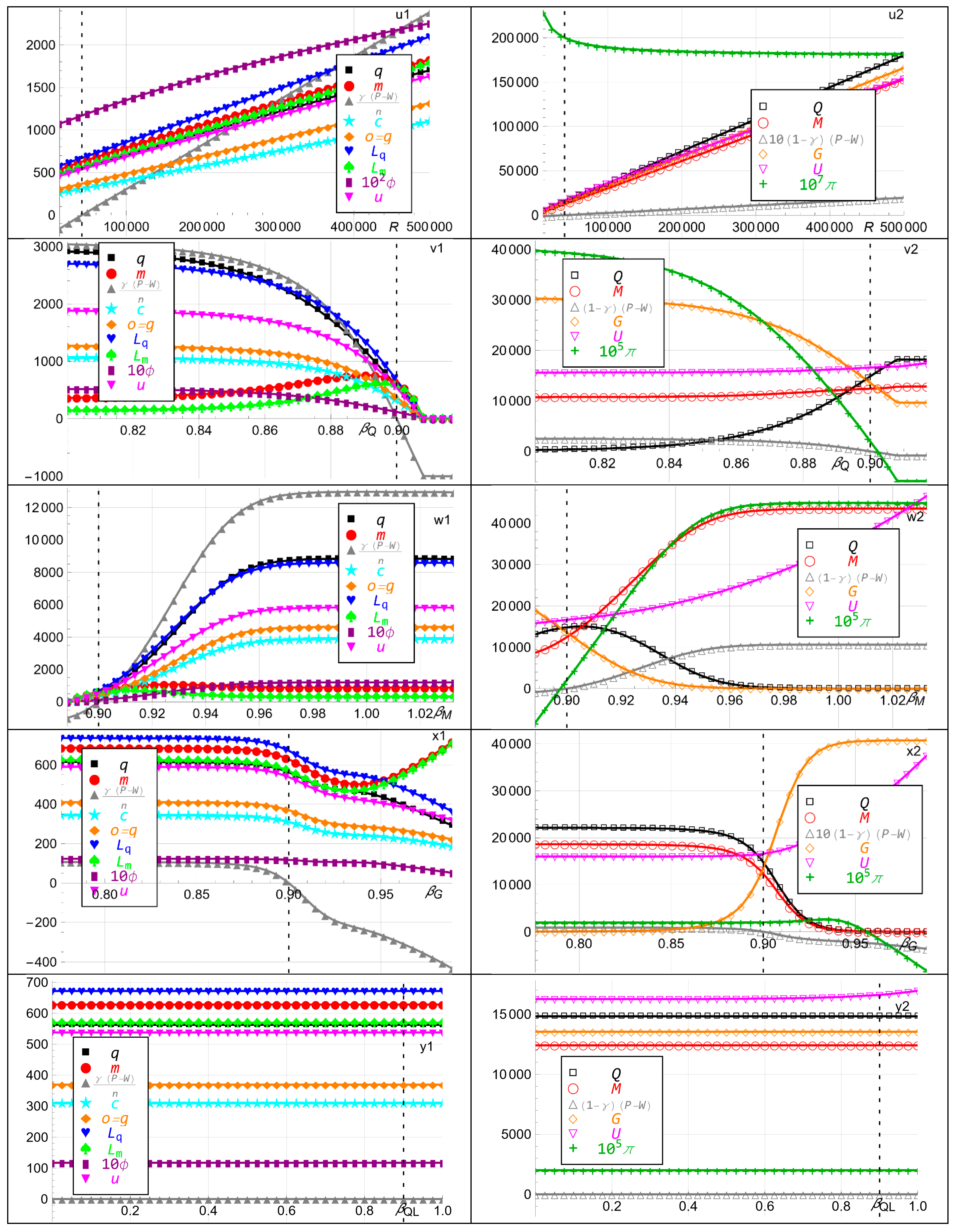
  • Increasing the bank’s fiat money exponent causes fiat money printing and inflation. The bank earns higher utility by holding more fiat money, eventually less hard money, and substantially less gold. The player’s variables including its utility increase, except its fiat money holding and fiat money loan, which first increase and eventually decrease. This shows that banks may strategically use fiat money printing to their advantage, even if it comes at the cost of long-term stability, as shown in Figure 2w.

7.2. Essential Insights

  • Increasing the player’s hard money borrowing interest rate induces the bank to withdraw fiat money. That causes the player to borrow more fiat money, which initially causes inflation, and also borrow more hard money because of the restrained allocation possibilities. That causes lower player utility and higher bank utility. Thus, higher hard money borrowing costs do not necessarily curb inflation but can instead fuel it, as shown in Figure 2f.
  • Increasing the player’s fiat money borrowing interest rate also induces the bank to withdraw fiat money. That causes the player to borrow more hard money, and also borrow more fiat money because of the restrained allocation possibilities. That causes inflation, lower player utility, and higher bank utility. Thus, higher fiat money borrowing costs also do not necessarily curb inflation but can instead fuel it, as shown in Figure 2g.
  • Increasing the bank’s hard money exponent in its utility causes fiat money withdrawal and decreased inflation. The bank earns higher utility by holding more hard money, slightly more fiat money, and substantially less gold. All the player’s variables including its utility decrease and eventually approach zero. This demonstrates the power banks have over inflation by strategically adjusting money supply and asset allocations, as shown in Figure 2v.

7.3. Insights

  • Increasing the player’s hard money holding exponent in its utility, and analogously for the other exponents, causes the player to allocate more resources to hard money, less and, eventually, nothing to everything else, and earn higher utility. The inflation decreases because the bank’s fiat money printing is offset by the player’s decreased borrowing, which causes lower bank utility, as shown in Figure 2j.
  • Increasing the player’s hard money loan exponent in its utility, and analogously for the other exponents, initially induces the player to borrow more hard money. That causes the bank to earn higher utility through withdrawing fiat money, which initially induces the player to also borrow fiat money, and earn lower utility, accompanied with inflation, as shown in Figure 2n.
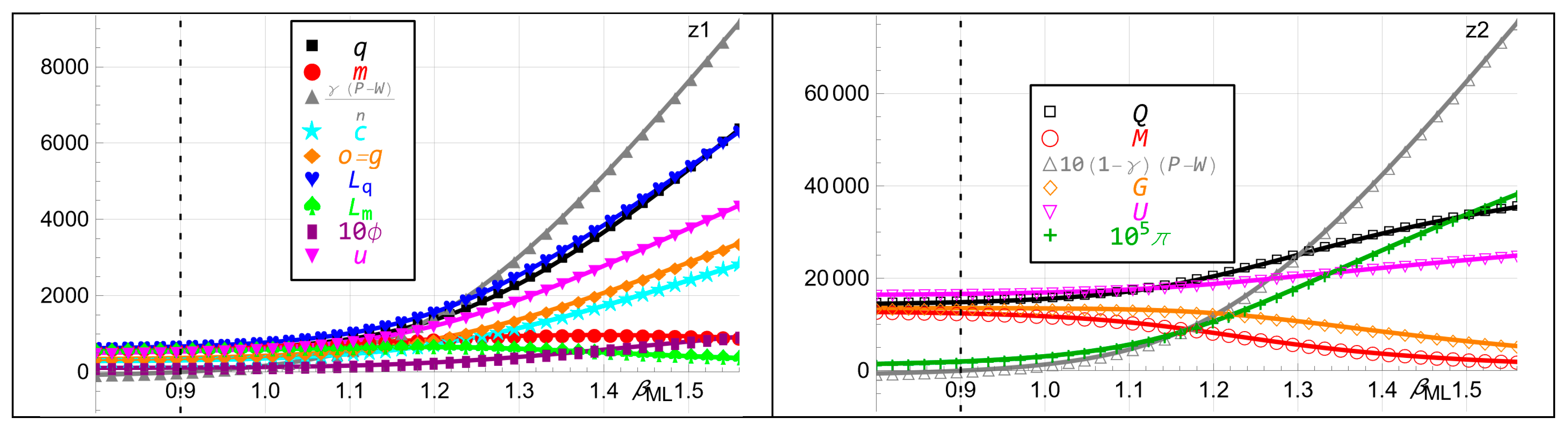
  • Increasing the bank’s fiat money loan exponent increases fiat money printing and inflation. The bank earns higher utility by holding more hard money and less fiat money and gold. The player earns higher utility by increasing all its variables except its fiat money holding and fiat money loan, which first increase and, eventually, decrease, as shown in Figure 2z.

8. Policy Implications for Central Banks

The findings of this study offer important policy implications for central banks managing fiat money printing and withdrawal. The strategic interactions between fiat and hard money highlight critical areas where central banks can intervene to maintain financial stability and monetary efficiency.

8.1. Inflation Control Through Strategic Money Printing and Withdrawal

  • Central banks should moderate fiat money printing to avoid excessive inflation, which can drive out hard money from circulation.
  • A balance between money supply expansion and contraction is necessary to prevent liquidity shortages that could harm borrowers and disrupt financial stability.
  • Policy tools such as open market operations and interest rate adjustments should be dynamically utilized to counter inflationary and deflationary risks.

8.2. Interest Rate Adjustments

  • Raising fiat money interest rates encourages fiat money printing and inflation, which may eliminate hard money from the financial system. Policymakers should manage this process carefully to avoid excessive inflationary pressure.
  • Higher hard money interest rates paradoxically constrain liquidity for players, benefiting the bank at the player’s expense. Thus, setting appropriate interest rates requires a balance between incentivizing fiat money use and ensuring economic stability.

8.3. Managing Money Supply in Multi-Currency Economies

  • In economies where hard and fiat money coexist, central banks must ensure monetary stability by adjusting the fiat supply based on inflationary trends.
  • Targeted money withdrawal strategies can be employed to reduce inflationary pressures while maintaining a stable financial environment.
  • Regulations surrounding the adoption of cryptocurrencies and hard money substitutes should be considered to prevent the destabilization of fiat currency systems.

8.4. Role of Transaction Costs in Currency Adoption

  • Policies that lower transaction costs for digital fiat currencies (e.g., CBDCs) can increase fiat money adoption while limiting inflation risks.
  • Higher transaction costs for hard money discourage its use, reinforcing fiat money dominance. Central banks should evaluate the impact of these costs on financial stability and economic efficiency.
  • Incentivizing digital payment adoption and improving infrastructure for digital currencies can reduce reliance on physical cash, further stabilizing monetary policy implementations.
By considering these policy implications, central banks can better manage the coexistence and competition between fiat and hard money, ensuring a more resilient and stable monetary environment.

9. Broader Macroeconomic Implications

The integration of digital currencies, including CBDCs and cryptocurrencies, has significant macroeconomic implications beyond national monetary policy. These impacts extend to global trade, capital flows, and financial stability, reshaping economic interactions at an international level.

9.1. Impact on Global Trade and Exchange Rates

  • Digital currencies can reduce exchange rate volatility by enabling faster and more stable cross-border transactions.
  • CBDCs and stablecoins could facilitate international trade by lowering remittance costs and improving financial efficiency.
  • Countries with well-established digital payment infrastructures may gain competitive advantages in global markets by reducing transaction delays and enhancing liquidity.

9.2. Shifts in Global Reserve Currencies

  • The rise in CBDCs could decrease reliance on traditional reserve currencies, such as the U.S. dollar, leading to a more multipolar financial system.
  • Digital currency adoption could shift the balance of financial power, allowing smaller economies to bypass conventional banking systems and access global liquidity directly.
  • The ability of CBDCs to settle transactions instantly and securely could enhance monetary sovereignty for emerging markets, reducing their vulnerability to external shocks.

9.3. Effects on Capital Flows and Financial Stability

  • Digital currencies could accelerate capital mobility, leading to increased financial volatility in economies with weak regulatory frameworks.
  • Large-scale digital currency transactions could facilitate capital flight from unstable economies, making them more susceptible to external financial shocks.
  • To mitigate these risks, central banks must establish robust financial stability measures, such as capital controls on digital asset transactions and international cooperation on regulatory standards.

9.4. Trade and Digital Payment Infrastructure

  • Countries investing in blockchain-based trade settlements could enhance trade efficiency and financial inclusion, benefiting exporters and importers.
  • Smart contract-based payment systems could automate trade agreements, reducing reliance on traditional banking intermediaries.
  • The expansion of decentralized finance (DeFi) and programmable money could enable seamless cross-border commerce, changing the dynamics of international business and monetary policy.
By addressing these broader macroeconomic implications, policymakers can better anticipate the long-term consequences of digital currency integration on the global financial landscape. Future research should explore how international cooperation on digital currency frameworks could mitigate risks while maximizing economic benefits.

10. Limitations and Future Research

One limitation of this article pertains to the nature of a money-in-utility function. Real-world financial decisions are influenced by a multitude of factors beyond just the amount of assets or consumption, e.g., expectations. Utility models should strive to account for these complexities to provide a more accurate representation of individual decision-making. Future research could expand the model’s scope regarding hard money. For instance, the hard money supply may be programmed through certain patterns, e.g., initial increase and subsequent decrease through burning. Future research could consider the integration of real-world data as an additional and valuable resource to corroborate the findings generated by the model. That could verify and enhance the model’s reliability and empirical support.
Another limitation is that inflation is only linked to fluctuations in fiat money creation, withdrawal, and loans. To advance the understanding of inflation, future research may integrate additional factors, e.g., money velocity and economic expectations. In economies with a fixed supply of hard money, price fluctuations caused by demand and supply shocks may cause instability. This implies that fiat money economies may persist due to their flexibility in managing the money supply to support growth and stability. Future research may explore the impact of shocks on inflation and strategic choices by the player and the bank. Future research may also introduce different types of players, e.g., borrowers, buyers, and sellers with different characteristics, potentially represented on [0,1] continuums. The consolidated bank can be divided into, e.g., central banks, commercial banks, and governments.
This article limits the analysis to hard and fiat money, consumption, other assets, and gold. Future research may introduce more asset types, e.g., stocks, bonds, and financial derivatives. Within the category resembling hard money, multiple kinds of cryptocurrencies like Bitcoin and minerals like gold may be modeled. Similarly, multiple kinds of fiat money may be modeled, e.g., paper money, coins, stablecoins, and CBDCs. To capture the time dimension, multi-period settings including repeated games may be analyzed, or evolutionary patterns may be explored to assess the potential coexistence of and competition between hard and fiat money. Methodologies such as replicator dynamics (Schuster & Sigmund, 1983; Wang & Hausken, 2021a) may be employed to model the evolution of multiple currencies over time. Future research may also consider additional factors beyond fiat money printing, withdrawal, inflation, and transaction costs, e.g., convenience, security, network effects, and monetary policy. Future research may also introduce more players and endogenize various model parameters, such as asset interest rates and borrowing interest rates.

11. Conclusions

A game-theoretic model involving hard and fiat money is analyzed between a representative player and a consolidated bank, which includes the central bank. Key takeaways are, first, that the control over the fiat money supply grants it a strategic advantage over the player, enabling it to reduce inflation through money withdrawal, often at the expense of player welfare. Second, increasing interest rates on hard money can paradoxically lower player utility because it prompts the bank to reduce fiat money supply, leading to liquidity constraints for the player. Third, rising interest rates on fiat money benefit both the player and the bank, encouraging fiat money printing and increasing inflation, ultimately driving hard money out of circulation. Fourth, the coexistence of hard and fiat money is fragile, as fiat money’s flexibility (printing and withdrawal) gives the bank long-term dominance in controlling inflation and shaping the economy.
The policy and macroeconomic implications of these findings have been explored in Section 8 and Section 9. Section 8 highlights how central banks can use money printing and withdrawal as strategic tools to manage inflation and liquidity constraints, while Section 9 discusses how these dynamics influence financial stability and the persistence of hard money.
The player chooses its holdings of hard and fiat money, consumption, other assets, gold, and loans in hard and fiat money. The bank chooses its holdings of hard and fiat money and gold. It also determines fiat money printing and withdrawal, which impacts the player. The inflation rate is determined by the bank’s fiat money printing and withdrawal, the player’s fiat money borrowing generated by money printing, and the amount of hard and fiat money in circulation. Hard and fiat money have different player transaction costs for consumption and buying other assets and gold.
The inflation rate decreases associated with the bank’s fiat money withdrawal when various characteristics of hard money become more favorable, such as a higher interest rate or a higher utility exponent for hard money for the bank. That benefits the bank but not the player. A higher utility exponent for hard money for the player also causes decreased inflation but is associated with the bank’s money printing, which compensates for the player’s decreased fiat money borrowing. Some paradoxical results arise. For example, an increased interest rate for hard money benefits the bank, which holds more hard money and less gold, and withdraws fiat money, causing decreased inflation, which causes the player to hold less hard money and receive lower utility. In contrast, the increased interest rate for fiat money benefits both the player and the bank through fiat money printing, despite increased inflation, eventually driving hard money out of existence. For a joint hard and fiat money economy, this illustrates how the bank may benefit at the expense of the player by regulating the fiat money supply through money printing and withdrawal.
With more players, the bank benefits from more fiat money loans. The bank withdraws fiat money and holds less hard and fiat money and gold. The inflation eventually decreases. The player’s allocation possibilities become constrained. The player thus eventually borrows and holds more fiat money, holds less hard money, and earns lower utility. As the hard money interest rate increases, the bank withdraws fiat money but benefits from increasing its hard money holding. The inflation decreases. The player’s constrained allocation possibilities decrease its utility and cause bankruptcy. In contrast, as the fiat money interest rate increases, the bank prints fiat money. Both the player and the bank benefit from increasing their fiat money holdings, inflation increases, and hard and fiat money eventually do not coexist. As the hard money or fiat money borrowing interest rate increases, the bank benefits from withdrawing fiat money, which constrains the player’s allocation possibilities, causing it to borrow both hard and fiat money.
As the player’s exponent in its utility for consumption, hard and fiat money, other assets, and gold increases, the player benefits from increasing the corresponding variable and decreasing its other variables. Less player borrowing causes lower utility for the bank. As the player’s exponent in its utility for hard money loans increases, the bank initially benefits from withdrawing fiat money. That causes the inflation and the player’s variables except its utility to be inverse U-shaped. The player is induced by the bank to borrow more, but eventually borrows less, and overall receives lower utility. As the player’s exponent in its utility for fiat money borrowing interest rate increases, the bank also initially benefits from withdrawing fiat money. That increases the inflation and causes the player’s fiat money borrowing and hard money holding to be inverse U-shaped. The player overall receives lower utility.
As the player’s transaction cost parameter values for hard and fiat money increase, the player’s transaction cost decreases. The player prefers to eventually hold more money of the kind with the lower transaction cost, allowing hard and fiat money to coexist. As the player’s other transaction cost-related parameters increase, the player’s transaction cost increases, causing less consumption, less holding of other assets and gold, more borrowing, and lower utility. The bank benefits from withdrawing more fiat money, and holds less hard and fiat money and gold.
As more printed fiat money is allocated to the player, the inflation increases. The player benefits from the joint presence of hard and fiat money and eventually borrows and holds less fiat money. The bank benefits from the player’s loans but does not benefit from its decreased fiat money allocation. As the bank’s exponent in its utility for hard money increases, it withdraws fiat money causing decreased inflation. The bank benefits from holding more hard money and less gold. The player becomes constrained and eventually receives zero utility. In contrast, as the bank’s exponent in its utility for fiat money increases, it prints fiat money, causing inflation. The bank benefits from holding more fiat money, less gold and, eventually, less hard money. The player benefits from increasing all its variables except its fiat money holding and fiat money loan, which eventually decrease. As the bank’s fiat money loan exponent in its utility increases, it prints fiat money, causing inflation. The bank benefits from holding more hard money, and less gold and fiat money. The player benefits from increasing all its variables except its fiat money holding and fiat money loan, which eventually decrease.
As the player benefits from more resources, the bank withdraws fiat money. That induces the player to borrow hard and fiat money, which benefits the bank causing inverse U-shaped inflation. As the bank benefits from more resources, the bank prints fiat money. The player benefits from increasing all its variables. The inflation decreases and levels out. The findings emphasize that transaction costs are a critical determinant of currency competition, influencing the adoption and viability of different monetary systems. This is particularly relevant for central bank digital currencies (CBDCs), which could alter the balance between fiat and hard money. A resourceful bank possesses greater potential for fiat money printing while keeping inflation under control.
The implications of this analysis extend beyond central banks to financial institutions and individual economic actors. Financial institutions must consider the strategic shifts in currency competition when assessing lending practices, liquidity management, and inflation hedging strategies. Meanwhile, individuals and businesses navigating a dual-currency economy must account for transaction costs, inflationary risks, and liquidity constraints when making financial decisions. Policymakers should anticipate how fiat money’s strategic advantages could impact financial stability and economic resilience, ensuring adaptive regulatory measures that mitigate excessive inflation and liquidity crises while promoting financial inclusion in digital and hybrid monetary environments.
This article’s findings underscore a fundamental truth in modern monetary systems: The power of fiat money printing and withdrawal grants central banks an unparalleled influence over financial stability and economic outcomes. While strategic interventions can curb inflation and enhance liquidity, they also risk constraining market participants and marginalizing alternative monetary assets. Policymakers must navigate this delicate balance, ensuring that fiat money dominance does not come at the cost of financial fragility. For financial institutions, understanding these strategic interactions is critical for optimizing asset allocation and mitigating inflationary risks. Meanwhile, individuals and businesses must recognize how central bank policies shape their financial realities, from borrowing costs to long-term wealth preservation. As the coexistence of fiat and hard money continues to evolve, the challenge remains: Will central banks adapt to this dual monetary landscape, or will their policies ultimately drive hard money out of existence?

Author Contributions

Conceptualization, K.H. and G.W.; methodology, K.H. and G.W.; software, K.H. and G.W.; validation, K.H. and G.W.; formal analysis, K.H. and G.W.; investigation, K.H. and G.W.; resources, K.H. and G.W.; data curation, K.H. and G.W.; writing—original draft preparation, K.H. and G.W.; writing—review and editing, K.H. and G.W.; visualization, K.H. and G.W.; supervision, K.H.; project administration, K.H. All authors have read and agreed to the published version of the manuscript.

Funding

This research received no external funding.

Informed Consent Statement

Not applicable.

Data Availability Statement

No new data were created or analyzed in this study. Data sharing is not applicable to this article.

Conflicts of Interest

The authors declare no conflict of interest.

Appendix A. Nomenclature

General parameters
n Number of players, n 1
I j Interest rate for asset j  determined by the open market, j = q , m , o , g ; I j R
r j The players’ borrowing interest rate for hard money and fiat money j ,   j = q , m ; r j R
Parameters for the player  i ,   i = 1 , , n
r The representative player’s resources, r 0
α j The player’s utility exponent   α j  for consumption and holding asset j ,   j = q , m , c , o , g α j 0
α j L The player’s utility exponent α j L for loans L j  in hard money and fiat money, j = q , m ;   α j L 0
σ j The player’s transaction cost parameter for hard money and fiat money, j = q , m ;   σ j 0
λ The player’s scaling exponent for consumption c , buying other assets o and gold g ,   λ 0
γ The fraction of fiat money helicopter airdrop/withdrawal allocated to the player, 0 γ 1
θ The scaling parameter of the player’s transaction cost, θ > 0
Parameters for the bank
R The bank’s resources,   R 0
β j The bank’s utility exponent β j  for holding asset j ,   j = Q ,   M ,   G ;   β j 0
β j L The bank’s utility exponent β j L for loan L j to the players,   j = q , m ;   β j L 0
Player i’s free-choice variables
j Player i ’s consumption and holding of assets, j = c , q , m , o ; j 0
L j Player i ’s hard money loan and fiat money loan L j ,   j = q , m ; L j 0
The bank’s free-choice variables
j The bank’s holding of hard money and fiat money, j = Q , M ;   j 0
P W The bank’s printing of fiat money minus the bank’s withdrawal of fiat money, P ,   W P 0 ,   W 0
Player i’s dependent variables
u The representative player’s utility, u 0
g = r q m c o + L q + L m + γ P W n The player’s holding of gold, g 0
The bank’s dependent variables
U The bank’s utility, U 0
G = R n L q + 1 γ P W Q M The bank’s holding of gold, G 0
The player’s and the bank’s dependent variables
π Inflation rate, π R
ϕ The player’s transaction cost, ϕ > 0

Appendix B. The Representative Player’s First-Order Conditions

u q = L m n L m + P W α m m 1 + I m m 1 + I m Q + M + n q + m Q + M + P W + n q + m + L m 1 + α m α m L 1 + r m L m 1 + r m Q + M + n q + m Q + M + P W + n q + m + L m 1 + α m L Q + M + P W + n q + m + L m 2 α g 1 + I g 1 + I g r + L q + L m + γ P W n q m c o 1 + α g + α q q 1 + I q α q q + θ λ r q m + L q + L m + γ P W n 1 + λ 1 + I q q σ q + 1 + I m m σ m + θ σ q q 1 + I q σ q r q m + L q + L m + γ P W n λ q 1 + I q q σ q + 1 + I m m σ m 2 = 0 , u m = α m 1 + I m m 1 + I m Q + M + n q + m Q + M + P W + n q + m + L m 1 + α m × m 2 + Q + M + m + n q + m Q + M + P W + n q + L m + m n 1 Q + M + P W + n q + m + L m 2 + α m L L m n L m + P W 1 + r m L m 1 + r m Q + M + n q + m Q + M + P W + n q + m + L m 1 + α m L Q + M + P W + n q + m + L m 2 α g 1 + I g 1 + I g r + L q + L m + γ P W n q m c o 1 + α g + θ λ r q m + L q + L m + γ P W n 1 + λ 1 + I q q σ q + 1 + I m m σ m + θ σ m m 1 + I m σ m r q m + L q + L m + γ P W n λ m 1 + I q q σ q + 1 + I m m σ m 2 = 0 , u c = α c c 1 + α c α g 1 + I g 1 + I g r + L q + L m + γ P W n q m c o 1 + α g = 0 , u o = α o 1 + I o o α o o α g 1 + I g 1 + I g r + L q + L m + γ P W n q m c o 1 + α g = 0 , u L q = α q L L q 1 + r q α q L L q + α g 1 + I g 1 + I g r + L q + L m + γ P W n q m c o 1 + α g θ λ r q m + L q + L m + γ P W n 1 + λ 1 + I q q σ q + 1 + I m m σ m = 0 , u L m = n L m m 1 + I m Q + M + n q + m Q + M + P W + n q + m + L m α m + α m L Q + M + n q + m L m Q + M + n m + q 1 + r m Q + M + P W + n q + m + L m α m L L m Q + M + P W + n q + m + L m + α g 1 + I g 1 + I g r + L q + L m + γ P W n q m c o 1 + α g θ λ r q m + L q + L m + γ P W n 1 + λ 1 + I q q σ q + 1 + I m m σ m = 0
Before the differentiation in (A1) for the representative player,  n q  and  n m  are replaced with  q + q e  and  m + m e , where  q e = n 1 q  and  m e = n 1 m  are constant for the  n 1  other players in the differentiation for the representative player. The parameter  q e 0  is the hard money held by the  n 1  players, i.e., all the  n  players except the one representative player. Similarly,  m e 0  is the fiat money held by the  n 1  players, i.e., all the  n  players except the one representative player. After the differentiation,  q e = n 1 q  and  m e = n 1 m  are inserted into the first-order conditions.

Appendix C. The Bank’s First-Order Conditions

U Q = β Q 1 + I q Q β Q Q β G 1 + I g 1 + I g R n L q + 1 γ P W Q M 1 + β G + n L m + P W β M 1 + I m Q + M + n q + m Q + M + P W + n q + m + L m β M + β M L n L m Q + M + n q + m 1 + r m Q + M + P W + n q + m + L m β M L Q + M + n q + m Q + M + P W + n q + m + L m = 0 , U M = 1 Q + M + P W + n q + m + L m 2 1 + I m 1 + I m Q + M + n q + m Q + M + P W + n q + m + L m 1 + β M + β M M n L m + P W + Q + M + n q + m Q + M + P W + n q + m + L m + β M L n L m n L m + P W 1 + r m n L m Q + M + n q + m 1 + r m Q + M + P W + n q + m + L m 1 + β M L β G 1 + I g Q + M + P W + n q + m + L m 2 × 1 + I g 1 + I g R n L q + 1 γ P W Q M 1 + β G = 0 , U P W = β M 1 + I m Q + M + n q + m Q + M + P W + n q + m + L m β M + β M L n L m Q + M + n q + m 1 + r m Q + M + P W + n q + m + L m β M L Q + M + P W + n q + m + L m β G 1 + I g 1 + γ 1 + I g R n L q + 1 γ P W Q M 1 + β G = 0

Appendix D. Interpretation of 14 of the Panels in Figure 2

In Figure 2d, as the interest rate  I o  of other assets increases through the benchmark  I o = 2 % , the player allocates more funds to other assets  o , which levels out when no further funds are available. The player’s fiat money holding  m  decreases and also levels out, and decreases more slowly than its hard money holding  q  in order to more effectively (since  σ m = 1.2 > σ q = 1  in (3)) constrain the increasing transaction cost  ϕ  associated with allocating to other assets  o . Thus, the player’s utility  u  increases. All the player’s other variables approach zero,  lim I o x = 0 x = q , c , g , L q , L m . The bank’s fiat money printing  P W  causes all its holdings to increase slightly, while its utility  U  decreases slightly. The inflation rate  π  is slightly U-shaped according to (7), where the variables counteract each other.
In Figure 2e, as the interest rate  I g  of gold increases through the benchmark  I g = 2 % , both the player and the bank allocate more funds to gold  G  and  g , which level out when no further funds are available. The player’s fiat money holding  m  decreases and also levels out, and decreases more slowly than its hard money holding  q  to constrain the increasing transaction cost  ϕ  associated with allocating to gold  g . Thus, the player’s utility  u  increases. All the player’s other variables approach zero,  lim I g x = 0 x = q , c , o , L q , L m . Contrary to Figure 2d, the bank withdraws fiat money shown with negative  P W . That causes the bank to decrease its holdings of hard money  Q  and fiat money  M  to decrease towards  lim I g Q = lim I g M = 0 , and it causes the inflation rate  π  to eventually go negative according to (7), while its utility  U  increases.
In Figure 2f, as the hard money borrowing interest rate  r q  increases moderately from  r q = 0 %  and above the benchmark  r q = 5 % , the player’s utility decreases from  u = 570.32  when  r q = 0 %  and goes negative when  r q > 16.94 % . The bank withdraws fiat money  P W  so strongly that its holdings first decrease slowly, and thereafter approach, i.e.,  lim r q x = 0 x = Q , M , G . Instead, it earns increasing utility  U  from loans  n L q  and  n L m . The eventually decreasing and negative inflation rate  π  detrimentally causes the player to incur both hard and fiat money loans  L q  and  L m  and, overall, increase its fiat money holding  m . The player’s consumption  c  and holdings of other assets  o  and gold  g  are inverse U-shaped and eventually approach  lim r q x = 0 x = c , o , g .
In Figure 2g, as the interest rate for borrowing fiat money  r m  increases moderately from  r m = 0 %  and above the benchmark  r m = 5 % , the player’s utility decreases from  u = 581.04  when  r m = 0 %  and goes negative when  r m > 29.98 % . The bank initially withdraws fiat money  P W  strongly, inducing the player to incur both hard and fiat money loans  L q  and  L m  and increase its fiat money holding  m . The player’s initially increasing fiat money borrowing  L m  outweighs the decreasing  P W , which causes an increasing inflation rate  π . The player’s consumption  c  and holdings of other assets  o  and gold  g  increase concavely until they reach constant levels. The bank’s holdings of fiat money  M  and gold  G  decrease toward zero. The player’s fiat money loan  L m  eventually becomes costly and decreases towards a constant. The bank’s negative money printing  P W  is thus initially U-shaped. The cheaper hard money loan  L q  increases towards an upper limit at the extremely high  r m = 203.00%, and is thereafter constant, since no more hard money  Q = 0  is available from the bank. That explains the kinks in the curves, including the bank’s inverse U-shaped utility  U  and the inverse U-shaped inflation rate  π , which eventually causes the bank’s negative money printing  P W  to be inverse U-shaped.
In Figure 2h, as the player’s resources  r  increases through the benchmark  r = 1000 , all its variables increase. The bank’s money withdrawal expressed with the negative and decreasing  P W  decreases the bank’s available funds, causing its holdings of hard money  Q , fiat money  M , and gold  G  to decrease. The bank earns increasing utility  U  due to the players’ increasing borrowing  n L q  and  n L m . The inflation rate  π  is slightly inverse U-shaped, as the bank’s fiat money withdrawal  P W  is offset by the players’ fiat money borrowing  n L m , as expressed in (7).
In Figure 2i, as the player’s exponent  α c  for consumption  c  increases through the benchmark  α c = 9 / 10 , it intuitively increases its consumption  c  logistically, and decreases its fiat money holding  m . Its utility  u  increases despite the increasing transaction cost  ϕ , and its other variables decrease;  lim α c x = 0 x = q , o , g , L q , L m . The bank prints fiat money  P W  and increases its holdings of hard money  Q , fiat money  M , and gold  G . Its utility  U  decreases due to the declining loans  n L q  and  n L m  from the players. The inflation rate  π  decreases since the increasing money printing  P W  is offset by the decreasing fiat money loans  n L m , according to (7).
In Figure 2j, as the player’s exponent  α q  for holding hard money  q  increases through the benchmark  α q = 9 / 10 , its hard money holding  q  intuitively increases logistically, causing its utility  u  to increase. Its other variables decrease;  lim α q x = 0 x = m , c , o , g , L q , L m , ϕ . The bank prints fiat money  P W , increases its holdings of fiat money  M  and gold  G , and decreases its hard money holding  Q . As in Figure 2i, the bank’s utility  U  and inflation rate  π  decrease.
In Figure 2k, as the player’s exponent  α m  for holding fiat money  m  increases through the benchmark  α m = 9 / 10 , its fiat money holding  m  intuitively increases logistically, causing its utility  u  to increase. Its other variables decrease;  lim α m x = 0 x = q , c , o , g , L q , L m , ϕ . The bank prints fiat money  P W , increases its holdings of fiat money  M  and gold  G , and decreases its hard money holding  Q . As in Figure 2i,j, the bank’s utility  U  and inflation rate  π  decrease.
In Figure 2l, as the player’s exponent  α o  for holding other assets  o  increases through the benchmark  α o = 9 / 10 , its other assets holding  o  intuitively increases logistically causing its transaction cost  ϕ  and utility  u  to increase, and its fiat money holding  m  decreases. Its other variables decrease;  lim α o x = 0 x = q , c , g , L q , L m . The bank prints fiat money  P W  and increases its holdings of hard money  Q , fiat money  M , and gold  G . As in Figure 2i–k, the bank’s utility  U  and inflation rate  π  decrease.
In Figure 2m, as the player’s exponent  α g  for holding gold  g  increases through the benchmark  α g = 9 / 10 , its gold holding  g  intuitively increases logistically, causing its transaction cost  ϕ  and utility  u  to increase. Its other variables decrease;  lim α g x = 0 x = q , c , o , L q , L m . The bank prints fiat money  P W  and increases its holdings of hard money  Q , fiat money  M , and gold  G . As in Figure 2i–l, the bank’s utility  U  and inflation rate  π  decrease.
In Figure 2n, as the player’s exponent  α q L  for a hard money loan  L q  increases above the benchmark  α q L = 9 / 10 , the bank withdraws fiat money substantially expressed with a negative  P W . That causes all the player’s variables to be inverse U-shaped and all the bank’s variables to be U-shaped, except the player’s utility  u , which is U-shaped, and the bank’s utility  U , which is inverse U-shaped. The player increases  L q  sharply towards a maximum when  α q L = 0.91 , and then decreases  L q  convexly and asymptotically towards  lim α qL L q = 0  as the hard money loan  L q  becomes too expensive. The inflation rate  π  is inverse U-shaped consistently with (7), particularly impacted by the inverse U-shaped fiat money loan  L m .
In Figure 2o, as the player’s exponent  α m L  for a fiat money loan  L m  increases above the benchmark  α m L = 9 / 10 , the bank withdraws fiat money expressed with a negative  P W . That causes the player’s hard money holding  q  and fiat money loan  L m  to be inverse U-shaped, and causes the player to increase all its other variables and earn negative utility  u < 0  when  α m L > 0.92 . The bank decreases its holdings of fiat money  M  and gold  G . Its hard money holding  Q  and utility U are inverse U-shaped. This causes the inflation rate  π  to increase consistently with (7), where the numerator increases more than the denominator decreases. The player’s fiat money holding  m  increases at a slower rate compared to its other assets  o  and gold  g  due to the player’s reduced willingness to hold fiat money  m  as the inflation rate  π  increases.
In Figure 2q, as the player’s transaction cost parameter  σ m  for fiat money  m  increases through the benchmark  σ m = 1.2 , the transaction cost  ϕ  of using fiat money  m  intuitively decreases as  σ m  appears in the denominator of the transaction cost function in (3). The player’s fiat money holding  m  is inverse U-shaped with a maximum when  σ m = 1.05 , and approaches a constant. The player’s hard money holding  q  decreases logistically towards a constant, while the player’s consumption  c  and holdings of other assets  o  and gold  g  increase logistically towards constants consistently, with the transaction cost approaching  lim σ q ϕ = 0 . The bank’s increasing fiat money printing  P W  induces the player to decrease its hard money loan  L q  and fiat money loan  L m , causing the bank to marginally increase its holdings of hard money  Q , fiat money  M , and gold  G , and earn marginally lower utility  U . The inflation rate  π  increases slightly, due to the many terms in (7) counteracting each other. As  σ m  decreases below  σ m = σ q = 1 , the player allocates substantially to hard money  q , according to (3), to limit the transaction cost  ϕ .
In Figure 2r, as the player’s transaction cost parameter  λ  increases through the benchmark  λ = 1.5 , the transaction cost  ϕ  intuitively increases as  λ  appears in the numerator of the transaction cost function in (3). Consequently, the player’s consumption  c , holdings of other assets  o , and gold  g  decrease concavely. The bank withdraws fiat money substantially expressed with a negative  P W . That causes the player to increase its other variables to limit its transaction cost  ϕ , and causes the bank to allocate less funds to hard money  Q , fiat money  M , and gold  G , and earn higher utility  U . The inflation rate  π  increases slightly.
In Figure 2t, as the player’s transaction cost scaling parameter  θ  increases through the benchmark  θ = 1 , the bank withdraws fiat money expressed with negative  P W , which causes the bank to decrease all its holdings and earn higher utility  U . The player responds by increasing its hard money loan  L q  and fiat money loan  L m , and also increase its holdings of hard money  q  and fiat money  m . The inflation rate  π  increases slightly, impacted positively by the players’ fiat money loan  n L m , and impacted negatively by  P W , according to (7). The player’s transaction cost  ϕ  increases overall, while its consumption  c , holdings of other assets  o , and gold  g  decrease. The player’s utility decreases and goes negative when  θ > 66.42 .
In Figure 2u, as the bank’s resources  R  increase through the benchmark  R = 41,485.53 , all variables for the player and the bank approach infinity;  lim R x = x = q , m , c , o , g , L q , L m , ϕ , Q , M , G , U . That causes the numerator and denominator in (7) to approach infinity, which causes the inflation rate to decrease convexly from  2.29 %  when  R = 12,060  towards  lim R π = 1.805 %  (numerical issues arise when  R < 12,060 .)
In Figure 2v, as the bank’s exponent for hard money  β Q  increases through the benchmark  β Q = 9 / 10 , the bank withdraws fiat money expressed with negative  P W . That causes the player to decrease all its variables except its fiat money holding  m  and fiat money loan  L m , which are inverse U-shaped, which means that they also eventually decrease. The bank intuitively increases its hard money holding  Q , which means, amplified by the fiat money withdrawal expressed with a negative  1 γ P W , that it has to decrease some of its other holdings. It chooses to decrease its gold holding  G  and increase its fiat money holding  M  marginally for the following reasons. The bank’s money withdrawal, combined with the player’s collapsing fiat money loans  L m  and increasing bank hard money holding  Q , cause the inflation rate  π  to decrease sharply according to (7) and become negative when  β Q > 0.902 . Conversely, as  β Q  decreases below the benchmark  β Q = 9 / 10 , the bank increasingly prints fiat money  P W . The player responds by increasing its hard money holding  q , and even increases its hard money loan  L q  to increase its consumption  c  and holdings  o = g  of other assets and gold. The player eventually decreases its fiat money holding  m  and fiat money loan  L m  due to the increasing inflation rate  π . The inverse U-shaped  m  and  L m  are due to the increasing inflation rate  π  as  β Q  decreases.
In Figure 2x, as the bank’s exponent for gold  β G  increases through the benchmark  β G = 9 / 10 , the bank intuitively increases its gold holding  G , and decreases its holdings of hard money  Q  and fiat money  M . That initially causes a slightly higher inflation rate  π  according to (7), which eventually becomes inverse U-shaped and goes negative because of the bank’s fiat money withdrawal expressed with a negative  P W . Decreased available funds cause the player to decrease all its variables except, eventually, its fiat money holding  m  and fiat money loan  L m , which are eventually U-shaped because of the deflation  π < 0  when  β G > 0.96 .
In Figure 2y, as the bank’s exponent  β Q L  for a fiat money loan  L Q  increases through the benchmark  β Q L = 9 / 10 , only the bank’s utility  U  increases according to (6). No other variables are impacted and remain constant.
In Figure 2z, as the bank’s exponent  β M L  for a fiat money loan  L m  increases through the benchmark  β M L = 9 / 10 , the bank increases its fiat money printing  P W . That causes an increasing inflation rate  π , which causes the bank to hold more hard money  Q , less fiat money  M , less gold, and earn slightly higher utility  U . Consequently, the player increases all its variables except its fiat money holding  m  and fiat money loan  L m , which are eventually inverse U-shaped because of the increasing inflation rate  π .

Note

1
Examples are feathers, bones, seashells, cloth, grain, silver, gold, metal coins, paper money, banknotes, and electronic money.

References

  1. Adrian, T., & Mancini-Griffoli, T. (2021). The rise of digital money. Annual Review of Financial Economics, 13, 57–77. [Google Scholar] [CrossRef]
  2. Alvarez, F., Argente, D., & Van Patten, D. (2022). Are cryptocurrencies currencies? Bitcoin as Legal Tender in El Salvador (Working Paper No. 29968). National Bureau of Economic Research. [Google Scholar]
  3. Ammous, S. (2018). The Bitcoin Standard: The decentralized alternative to central banking. John Wiley & Sons. [Google Scholar]
  4. Ammous, S., & D’Andrea, F. A. M. C. (2022). Hard money and time preference: A Bitcoin perspective. MISES: Interdisciplinary Journal of Philosophy, Law and Economics, 10, 1–17. [Google Scholar] [CrossRef]
  5. Asimakopoulos, S., Lorusso, M., & Ravazzolo, F. (2019). A new economic framework: A DSGE model with cryptocurrency (Working Paper. No.07/2019). Centre for Applied Macro- and Petroleum Economics. [Google Scholar]
  6. Ayadi, A., Ghabri, Y., & Guesmi, K. (2023). Directional predictability from central bank digital currency to cryptocurrencies and stablecoins. Research in International Business and Finance, 65, 101909. [Google Scholar] [CrossRef]
  7. Ba, C. T., Clegg, R. G., Steer, B. A., & Zignani, M. (2024). Investigating shocking events in the ethereum stablecoin ecosystem through temporal multilayer graph structure. arXiv, arXiv:2407.10614. [Google Scholar]
  8. Badev, A., & Watsky, C. (2023). Interconnected Defi: Ripple effects from the Terra collapse (Finance and Economics Discussion Series 2023-044). Board of Governors of the Federal Reserve System. [Google Scholar]
  9. Benchimol, J., & Fourçans, A. (2012). Money and risk in a Dsge framework: A bayesian application to the Eurozone. Journal of Macroeconomics, 34(1), 95–111. [Google Scholar] [CrossRef]
  10. Benigno, P., Schilling, L. M., & Uhlig, H. (2022). Cryptocurrencies, currency competition, and the impossible trinity. Journal of International Economics, 136, 103601. [Google Scholar] [CrossRef]
  11. Bibi, S. (2023). Money in the time of Crypto. Research in International Business and Finance, 65, 101964. [Google Scholar] [CrossRef]
  12. Boissay, F., Cornelli, G., Doerr, S., & Frost, J. (2022). Blockchain scalability and the fragmentation of Crypto (No. 56). Bank for International Settlements. Available online: https://www.bis.org/publ/bisbull56.pdf (accessed on 2 March 2025).
  13. Bordo, M. D. (1983). Some aspects of the monetary economics of richard cantillon. Journal of Monetary Economics, 12(2), 235–258. [Google Scholar] [CrossRef]
  14. Bordo, M. D., Dittmar, R. D., & Gavin, W. T. (2007). Gold, fiat money, and price stability. The BE Journal of Macroeconomics, 7(1). Available online: https://www.degruyter.com/document/doi/10.2202/1935-1690.1525/html (accessed on 2 March 2025).
  15. Bordo, M. D., & Vegh, C. A. (2002). What if alexander hamilton had been Argentinean? A comparison of the early monetary experiences of Argentina and the United States. Journal of Monetary Economics, 49(3), 459–494. [Google Scholar] [CrossRef]
  16. Briola, A., Vidal-Tomás, D., Wang, Y., & Aste, T. (2022). Anatomy of a Stablecoin’s failure: The Terra-Luna case. arXiv, arXiv:2207.13914. [Google Scholar] [CrossRef]
  17. Caginalp, C., & Caginalp, G. (2019). Establishing cryptocurrency equilibria through game theory. AIMS Mathematics, 4(3), 420–436. [Google Scholar] [CrossRef]
  18. Chen, M., Wu, J., Jeon, B. N., & Wang, R. (2017). Monetary policy and bank risk-taking: Evidence from emerging economies. Emerging Markets Review, 31, 116–140. [Google Scholar] [CrossRef]
  19. Chiu, J., Davoodalhosseini, S. M., Jiang, J., & Zhu, Y. (2023). Bank market power and central bank digital currency: Theory and quantitative assessment. Journal of Political Economy, 131(5), 1213–1248. [Google Scholar] [CrossRef]
  20. Chu, A. C., & Lai, C. C. (2013). Money and the welfare cost of inflation in an R&D growth model. Journal of Money, Credit and Banking, 45(1), 233–249. [Google Scholar]
  21. Cong, L. W., & Mayer, S. (2022). The coming battle of digital currencies (The SC Johnson College of Business Applied Economics and Policy Working Paper Series, No. 2022-04). SC Johnson. [Google Scholar] [CrossRef]
  22. Cooper, R. N., Dornbusch, R., & Hall, R. E. (1982). The gold Standard: Historical facts and future prospects. Brookings Papers on Economic Activity, 1982(1), 1–56. [Google Scholar] [CrossRef]
  23. Doan Van, D. (2020). Money supply and inflation impact on economic growth. Journal of Financial Economic Policy, 12(1), 121–136. [Google Scholar] [CrossRef]
  24. Dubey, P., & Geanakoplos, J. (2003). Inside and outside fiat money, gains to trade, and Is-Lm. Economic Theory, 21, 347–397. [Google Scholar] [CrossRef]
  25. Engineer, M. (2000). Currency transactions costs and competing fiat currencies. Journal of International Economics, 52(1), 113–136. [Google Scholar] [CrossRef]
  26. Feenstra, R. C. (1986). Functional equivalence between liquidity costs and the utility of money. Journal of Monetary Economics, 17(2), 271–291. [Google Scholar] [CrossRef]
  27. Feres, A. (2021). Fiat, debt, & inflation: Has the federal reserve financially enslaved our great nation? (28720363) [Doctoral dissertation, Utica College]. Available online: https://www.proquest.com/openview/8a827460ee3c936c14eeb17a276f1f00/1?pq-origsite=gscholar&cbl=18750&diss=y (accessed on 2 March 2025).
  28. Fernández-Villaverde, J., & Sanches, D. (2019). Can currency competition work? Journal of Monetary Economics, 106, 1–15. [Google Scholar] [CrossRef]
  29. Fernández-Villaverde, J., & Sanches, D. (2023). A model of the gold Standard. Journal of Economic Theory, 214, 105759. [Google Scholar] [CrossRef]
  30. Ferrari Minesso, M., Mehl, A., & Stracca, L. (2022). Central bank digital currency in an open economy. Journal of Monetary Economics, 127, 54–68. [Google Scholar] [CrossRef]
  31. Ferretti, S., & Furini, M. (2024). Cryptocurrency turmoil: Unraveling the collapse of a Unified Stablecoin (Ustc) through Twitter as a passive sensor. Sensors, 24(4), 1270. [Google Scholar] [CrossRef]
  32. Fisher, I. (1911). The purchasing power of money: Its determination and relation to credit, interest, and crises. Macmillan. [Google Scholar]
  33. Fisher, I. (1920). The Purchasing Power of Money: Its Determination and Relation to Credit, Interest and Crises (New and revised edition). Macmillan Company. Available online: https://fraser.stlouisfed.org/title/3610 (accessed on 2 March 2025).
  34. Forbes Advisor. (2024). Credit card processing fees: The ultimate guide. Available online: https://www.forbes.com/advisor/business/credit-card-processing-fees/ (accessed on 2 March 2025).
  35. Fu, S., Wang, Q., Yu, J., & Chen, S. (2022). Rational ponzi games in Algorithmic stablecoin. arXiv, arXiv:2210.11928. [Google Scholar]
  36. Gertler, M., & Kiyotaki, N. (2015). Banking, liquidity, and bank runs in an infinite horizon economy. American Economic Review, 105(7), 2011–2043. [Google Scholar] [CrossRef]
  37. Hayakawa, H. (1992). The non-neutrality of money and the optimal monetary growth rule when preferences are recursive: Cash-in-advance vs. money in the utility function. Journal of Macroeconomics, 14(2), 233–266. [Google Scholar] [CrossRef]
  38. Itaya, J. I., & Mino, K. (2003). Inflation, transaction costs and indeterminacy in monetary economies with endogenous growth. Economica, 70(279), 451–470. [Google Scholar] [CrossRef]
  39. Johnson, M. (2023). Is Zimbabwe’s recently released gold-backed digital currency a good idea? Available online: https://internationalbanker.com/brokerage/is-zimbabwes-recently-released-gold-backed-digital-currency-a-good-idea/ (accessed on 2 March 2025).
  40. Jumde, A., & Cho, B. Y. (2020). Can cryptocurrencies overtake the fiat money? International Journal of Business Performance Management, 21(1–2), 6–20. [Google Scholar] [CrossRef]
  41. Keister, T., & Sanches, D. (2023). Should central banks issue digital currency? The Review of Economic Studies, 90(1), 404–431. [Google Scholar] [CrossRef]
  42. Kim, T. (2017). On the transaction cost of Bitcoin. Finance Research Letters, 23, 300–305. [Google Scholar] [CrossRef]
  43. Kosse, A., & Mattei, I. (2023). Making headway—Results of the 2022 Bis survey on central bank digital currencies and crypto (Paper No. 136). Bank for International Settlements. Available online: https://www.bis.org/publ/bppdf/bispap136.htm (accessed on 2 March 2025).
  44. Kwon, Y., Pongmala, K., Qin, K., Klages-Mundt, A., Jovanovic, P., Parlour, C., Gervais, A., & Song, D. (2023). What drives the (in)stability of a stablecoin? arXiv, arXiv:2307.11754. [Google Scholar]
  45. Laboure, M., H.-P. Müller, M., Heinz, G., Singh, S., & Köhling, S. (2021). Cryptocurrencies and Cbdc: The route ahead. Global Policy, 12(5), 663–676. [Google Scholar] [CrossRef]
  46. Lagos, R., Rocheteau, G., & Wright, R. (2017). Liquidity: A new monetarist perspective. Journal of Economic Literature, 55(2), 371–440. [Google Scholar] [CrossRef]
  47. Lan, B., Zhuang, L., & Zhou, Q. (2023). An evolutionary game analysis of digital currency innovation and regulatory coordination. Mathematical Biosciences and Engineering, 20(5), 9018–9040. [Google Scholar] [CrossRef]
  48. Long, S., Pei, H., Tian, H., & Lang, K. (2021). Can both Bitcoin and gold serve as safe-haven assets?—A comparative analysis based on the Nardl model. International Review of Financial Analysis, 78, 101914. [Google Scholar] [CrossRef]
  49. Mansoorian, A., & Michelis, L. (2005). Money, habits and growth. Journal of Economic Dynamics and Control, 29(7), 1267–1285. [Google Scholar] [CrossRef]
  50. Martin, A., & Schreft, S. L. (2006). Currency competition: A partial vindication of hayek. Journal of Monetary Economics, 53(8), 2085–2111. [Google Scholar] [CrossRef]
  51. Masciandaro, D., & Volpicella, A. (2016). Macro prudential governance and central banks: Facts and drivers. Journal of International Money and Finance, 61, 101–119. [Google Scholar] [CrossRef]
  52. McCallum, B. T. (1997). Crucial issues concerning central bank independence. Journal of Monetary Economics, 39(1), 99–112. [Google Scholar] [CrossRef]
  53. Mian, A., Straub, L., & Sufi, A. (2021). A goldilocks theory of fiscal policy. NBER Working Paper, No.w29351. National Bureau of Economic Research. [Google Scholar]
  54. Mishra, B., & Prasad, E. S. (2024). A simple model of a central bank digital currency. Journal of Financial Stability, 73, 101282. [Google Scholar] [CrossRef]
  55. Nabilou, H. (2020). Testing the waters of the rubicon: The European central bank and central bank digital currencies. Journal of Banking Regulation, 21(4), 299–314. [Google Scholar] [CrossRef]
  56. Nakamoto, S. (2008). Bitcoin: A peer-to-peer electronic cash system. Available online: https://bitcoin.org/bitcoin.pdf (accessed on 2 March 2025).
  57. Nicholson, J. S. (1888). A treatise on money and essays on present monetary problems. William Blackwood and Sons. [Google Scholar]
  58. Nyathi, L. D., & Mutale, J. (2025). Perceptions of the Zimbabwe Gold Currency (Zig) as a Panacea to economic stability. International Journal of Research and Innovation in Social Science, 9(15), 80–91. [Google Scholar] [CrossRef]
  59. Oh, E. Y., & Zhang, S. (2022). Informal economy and central bank digital currency. Economic Inquiry, 60(4), 1520–1539. [Google Scholar] [CrossRef]
  60. Rocheteau, G., & Nosal, E. (2017). Money, payments, and liquidity. MIT Press. [Google Scholar]
  61. Rolnick, A. J., & Weber, W. E. (1997). Money, inflation, and output under fiat and commodity standards. Journal of Political Economy, 105(6), 1308–1321. [Google Scholar] [CrossRef]
  62. Sakurai, Y., & Kurosaki, T. (2023). Have cryptocurrencies become an inflation hedge after the reopening of the U.S. economy? Research in International Business and Finance, 65, 101915. [Google Scholar] [CrossRef]
  63. Saygılı, H. (2012). Consumption (in) Efficiency and financial account management. Bulletin of Economic Research, 64(3), 319–333. [Google Scholar] [CrossRef]
  64. Scharnowski, S. (2022). Central bank speeches and digital currency competition. Finance Research Letters, 49, 103072. [Google Scholar] [CrossRef]
  65. Schilling, L. M., & Uhlig, H. (2019). Currency substitution under transaction costs. AEA Papers and Proceedings, 109, 83–87. [Google Scholar] [CrossRef]
  66. Schmitt-Grohé, S., & Uribe, M. (2004). Optimal fiscal and monetary policy under sticky prices. Journal of Economic Theory, 114(2), 198–230. [Google Scholar] [CrossRef]
  67. Schuster, P., & Sigmund, K. (1983). Replicator dynamics. Journal of Theoretical Biology, 100(3), 533–538. [Google Scholar] [CrossRef]
  68. Senner, R., & Sornette, D. (2019). The holy grail of crypto currencies: Ready to replace fiat money? Journal of Economic Issues, 53(4), 966–1000. [Google Scholar] [CrossRef]
  69. Steiner, W. H. (1941). Money and banking. H. Holt and Company. [Google Scholar]
  70. Vázquez, J. (1998). How high can inflation get during hyperinflation? A transaction cost demand for money approach. European Journal of Political Economy, 14(3), 433–451. [Google Scholar] [CrossRef]
  71. Wang, G., & Hausken, K. (2021a). Conventionalists, pioneers and criminals choosing between a national currency and a global currency. Journal of Banking and Financial Economics, 2(16), 104–133. [Google Scholar] [CrossRef]
  72. Wang, G., & Hausken, K. (2021b). Governmental taxation of households choosing between a national currency and a cryptocurrency. Games, 12(2), 34. [Google Scholar] [CrossRef]
  73. Wang, G., & Hausken, K. (2022a). Competition between variable–supply and fixed–supply currencies. Economies, 10(11), 270. [Google Scholar] [CrossRef]
  74. Wang, G., & Hausken, K. (2022b). The evolution of fixed-supply and variable-supply currencies. Humanities & Social Sciences Communications, 9, 137. [Google Scholar] [CrossRef]
  75. Wang, G., & Hausken, K. (2022c). A game between central banks and households involving central bank digital currencies, other digital currencies and negative interest rates. Cogent Economics & Finance, 10(1), 2114178. [Google Scholar] [CrossRef]
  76. Wang, G., & Hausken, K. (2024). Hard money and fiat money in an inflationary world. Research in International Business and Finance, 67, 102115. [Google Scholar] [CrossRef]
  77. Wang, Y., Wei, Y., Lucey, B. M., & Su, Y. (2023). Return spillover analysis across central bank digital currency attention and cryptocurrency markets. Research in International Business and Finance, 64, 101896. [Google Scholar] [CrossRef]
  78. Welburn, J. W., & Hausken, K. (2017). Game theoretic modeling of economic systems and the european debt crisis. Computational Economics, 49(2), 177–226. [Google Scholar] [CrossRef]
  79. Wen, F., Tong, X., & Ren, X. (2022). Gold or bitcoin, which is the safe haven during the COVID-19 pandemic? International Review of Financial Analysis, 81, 102121. [Google Scholar] [CrossRef] [PubMed]
  80. World Gold Council. (2024). Gold production by country 2024–Report. Available online: https://www.gold.org/goldhub/data/gold-production-by-country (accessed on 2 March 2025).
  81. Yu, Z. (2023). On the coexistence of cryptocurrency and fiat money. Review of Economic Dynamics, 49, 147–180. [Google Scholar] [CrossRef]
  82. Zhang, J. (2000). Inflation and growth: Pecuniary transactions costs and qualitative equivalence. Journal of Money, Credit and Banking, 1–12. [Google Scholar] [CrossRef]
Figure 1. Flows of funds with blue one-way solid arrows between the bank, the representative player, and the  n 1  other players, and how they strategically allocate their sources of funds. Red two-way dashed arrows denote the players’ allocation. Green two-way dashed arrows denote the bank’s allocation.
Economies 13 00080 g001
Table 1. The player’s variables, the bank’s variables, and the inflation rate  π  for the 26 panels in Figure 2, where “ ” expresses a decrease, “ ” expresses an increase, “ ” expresses a U-shaped pattern, “ ” expresses an inverse U-shaped pattern, “ ” expresses a sequence of U-shaped and inverse U-shaped patterns, “ = ” expresses constancy, and “ ” expresses approximate constancy.
Figure 2The Player’s VariablesThe Bank’s Variables
q m γ ( P W ) n c o g L q L m ϕ u Q M ( 1 γ ) ( P W ) G U π
a n
b I q
c I m
d I o
e I g
f r q
g r m
h r
i α c
j α q
k α m
l α o
m α g
n α q L
o α m L
p σ q
q σ m
r λ
s γ
t θ
u R
v β Q
w β M
x β G
y β Q L = = = = = = = = = = = = = = =
z β M L
Disclaimer/Publisher’s Note: The statements, opinions and data contained in all publications are solely those of the individual author(s) and contributor(s) and not of MDPI and/or the editor(s). MDPI and/or the editor(s) disclaim responsibility for any injury to people or property resulting from any ideas, methods, instructions or products referred to in the content.

