How Harmful Is a High Share of Public Expenditure in GDP?

Abstract

We aim to analyze the potential positive or negative effects of public expenditure on economic growth, as well as their determinants. To this goal, we use a simple theoretical model, which has the specificity to distinguish between public investment and consumption expenditure, and which could be applied to a wide range of developed or developing countries. Regarding public spending, we find that public consumption expenditure usually harms global economic growth, whereas public investment expenditure benefits economic activity: it can increase income per head, provided real returns on capital are not too small. We can also theoretically underline the existence of an inverted U-shaped relation between the variation of public investment or consumption expenditure and economic growth. An increase in public spending would benefit economic growth only up to a maximal variation, which positively depends on real capital returns, but negatively depends on the capitalization of the economy. Regarding fiscal resources, we find that increasing the consumption taxation rate and the share of fiscal resources collected through consumption taxes could benefit global economic growth, even if it is detrimental to private consumption.

1. Introduction

A worldwide tendency was the huge increase of the share of public expenditure in GDP during the XXe century, from around 10% of GDP on average in 1900 to 40% on average and even more than 50% of GDP in some Organization for Economic Cooperation and Development (OECD) countries in 2000: higher provision of public goods and services, stronger transfers. This can be due to the increasing demand for social services in more developed countries (Wagner law), to the higher facility for politicians to increase public expenditure and budget deficits rather than reduce social benefits. Therefore, economic analysis has been conducted to determine whether this public expenditure growth benefits or harms economic growth. However, the effect of the global size of public spending can then be distinguished from the effect of the structure of this public spending.

The link between government size and economic growth is not unambiguous. First, public expenditure can benefit economic growth, as public consumption is one explicit element of final consumption in calculating the Growth Domestic Product Indicator. By fiscal multipliers, increasing public expenditure (infrastructure, Research and Development, health, education) can imply an increase more than proportional in final production and global economic activity. A reverse causality explanation of the positive link is that higher economic growth implies higher fiscal revenues (VAT or personal taxes). However, with the eviction effect, high public expenditure can also increase interest rates and harm the more productive private investment and private consumption. Higher taxation rates to finance public expenditure can reduce the returns to investment, the productivity and the incentive to invest and to produce. A reverse causality explanation can also justify the negative link between the size of the government and economic growth. In case of weaker economic growth or recession, automatic stabilizers and fiscal transfers such as unemployment provisions, must increase to compensate for the weaker purchasing power of households.

Since 2005, France and Denmark have the highest share of public expenditure in GDP. For example, reaching 57.5% of GDP in 2024, total public general expenses in France are the highest in the European Union and nearly 10 percentage points above the European average (49.2%). The high level of public expenditure in France is due to social spending, and to the large degree of risk socialization: mainly retirement expenditure, but also housing subsidies, family allowances, and health. A high level of public spending is not a problem in itself, as it can mostly reflect different choices in the socialization of certain types of spending (pensions, healthcare, education, etc.). For example, in the Scandinavian countries, a high level of public expenditure is not a problem as underlying policies and institutions are mainly efficient. Nevertheless, it can become a problem when high public spending reflects inefficient public policies, when revenues cannot be increased to balance the budget, thereby putting debt sustainability at risk, or when the level of public spending limits the space available to respond to large macroeconomic shocks. The problem is when structural public expenditure is too high, hindering productive investment for the future (ecological transition, artificial intelligence). Public expenditure covers collective public spending (police, security, public administration, etc.) and insurance transfers (healthcare, pensions system, unemployment benefits). In the Bismarkian tradition, the insurance transfer system was initially based on individual contributions qualifying for benefits. Nevertheless, because of a lack of fiscal resources and high budget deficits, in the Beveridgian tradition, even the insurance system was, over time, more and more often forced to be financed with taxes and by collectivity. To variable degrees, countries have introduced minimum pension payments and free minimal health service provision. It is mainly for these social protection expenditures (social welfare, health, education) that the gap is large between France, Denmark, Sweden, Finland, and other developed countries.

Economic development is limited without a government insuring property rights and the furniture of public goods such as infrastructures, social services, health, or education. But economic growth is also limited with an overwhelming government preventing the development of private initiative, as public goods have diminishing returns. An excessive increase in public expenditure is dangerous for the sustainability of public finances. The budget deficit and the public debt must be contained at a time when there are pressures on these public finances because of demographic trends (spending on pensions and long-term care with a higher life expectancy). Public spending is highly necessary but must be used efficiently and in the most productive way: to improve long-term growth perspectives, considering equity considerations. The goal is to achieve better outcomes at a sustainable level of public spending. A balance has to be drawn between reducing public indebtedness, cutting taxes, and financing public investment in key areas.

Cepparulo and Mourre (2020) provide a survey of the literature on the effect of composition and size of public expenditure. In terms of size, public spending would be either beneficial in the Keynesian literature to sustain global demand in the short-term, or harmful in the classical tradition because of the crowding-out effect on private investment in the medium term. There is a large amount of economic literature on the impact of government size on economic growth. Theoretical as well as empirical analysis would tend to conclude that public expenditure would be necessary and beneficial up to a certain share in a percentage of GDP. More precisely, the ‘Armey Curve’ mentions that public spending would be beneficial up to a maximal point; however, it would become harmful thereafter (see the following Section 2). The majority of the empirical literature supports the existence of such an inverted U-shaped relation with a maximal level of public expenditure beyond which it can become harmful. Even if public spending is beneficial, beyond a certain point, the diminishing returns of public capital, the eviction effect of more productive private investment because of high interest rates, as well as bureaucratic inefficiencies tend to dominate. In terms of composition, according to endogenous growth theory and empirical observations, productive public investment (physical capital accumulation, but also human capital: education or research) could have a positive effect on growth, contrary to operating expenditures: current spending, government consumption, or subsidies. The efficacy of public spending could also depend on its financing and the soundness of public finances: budget deficit and public debt.

Our paper confirms the benefits of public investment expenditure for economic growth, as well as the harmfulness of public consumption expenditure. We also prove theoretically the existence of an inverted U-shaped relation between increasing public expenditure and economic growth, as well as the correlative existence of an optimal size of the government. These results have already been mentioned in the theoretical or empirical literature. However, the main contribution of our modeling is to highlight the theoretical determinants of this optimal size of the government and to shed light on the precise determinants of such a threshold, which should be useful to policymakers. The efficacy of higher public spending seems to depend, in particular, on the real interest rate, but could also be related to the capital share in the production function, or to the preference of households for public services. To derive such indications, Section 2 partially reviews the economic literature. Section 3 explains our theoretical modeling. Section 4 provides theoretical results on the effect of public investment and consumption expenditure on economic growth, on the determinants of the efficacy of public spending, and on the adequate repartition between consumption, labor, and capital taxation rates to collect these fiscal resources. Section 5 concludes the paper.

2. A Brief Review of Economic Literature

The government provides intermediate goods necessary in the production process, investment goods improving production capacities, but also final public consumption goods. It provides public goods that the market cannot provide efficiently, and it removes distortions in the allocation of resources due to externalities. Therefore, the link between public expenditure and short-run or long-run economic growth has long been studied in the economic literature [see, for example, Forte and Magazzino (2011), Chobanov and Mladenova (2009) or Cenc (2022) for a literature review].

A too-low level of public expenditure would not allow the State to guarantee the proper functioning of the economy, whereas an excessively high level of public expenditure would discourage a sufficient investment in the private sector because of the high fiscal burden. When the public sector is small, it can contribute to increasing the productivity of capital. However, when the size of the public sector is very high, it can crowd out more productive private investment. Moreover, governmental activities would have diminishing returns and their productivity could become too low beyond a certain level. The government could begin to be involved in activities for which it is ill-suited in comparison with the market. Public activities can also sometimes be conducted by interest groups to the detriment of global social welfare. So, Bergh and Henrekson (2011) underline that there is a negative relation between the size of the government and economic growth in many economic studies.

More precisely, regarding the composition of public spending, public expenditure is classified into ten primary expenditure items1 plus interest payments. Then, the productivity of various public expenditures and the structure of public spending seem to impact the consequences of the share of public expenditure in GDP on economic growth. Indeed, productive (unproductive) public expenditures are more likely to have a positive (negative) effect on economic growth. Nevertheless, Cepparulo and Mourre (2020) show that growth-friendly spending (education, R&D, health, transport, and communication infrastructures) only represents a third of total expenditure in the European Union. Therefore, the negative effect on economic growth of public spending beyond a certain level would correspond to the fact that as public spending increases, the share of unproductive public expenditure is proportionally higher. Kutasi and Marton (2020) analyze the correlation between various types of public expenditures and GDP growth in 25 EU countries in the period 1996–2017. They find that social protection or general public service harms GDP growth, whereas lagged education and health positively impact GDP growth.

Fournier and Johansson (2016) observed a large panel of countries between 1987 and 2014. They find that some public spending items (public investment, health, research and development, educational level) boost potential growth, while others (pensions and public subsidies) lower potential growth. There is also evidence that too large governments reduce long-term potential growth, unless the functioning of government is highly effective (as in Nordic countries), with a high trust of citizens in the government, a low level of corruption, and more decentralization. In this context, the Swedish public expenditure mix could appear the most growth-friendly among the OECD countries. Bergh and Henrekson (2011) show that some countries with high taxes can enjoy above-average growth, such as Scandinavian countries, particularly Sweden. Indeed, by implementing market-friendly policies, countries with higher social trust levels can develop larger government sectors without harming the economy.

Fölster and Henrekson (2001), Fall and Fournier (2015), and Cenc (2022) find robust negative econometric correlations between growth and total government expenditure. In a panel of 29 OECD equally rich countries, between 1970 and 2005, Bergh and Karlsson (2010) also show that government size robustly correlates negatively with growth, even when controlling for economic freedom and globalization. However, they also find some evidence that countries with big governments can use economic openness and sound economic policies to mitigate the negative effects of big governments. In the same way, for 11 Central and Eastern European countries, Mitu and Stanciu (2023) find that expenditure performance, as well as efficiency scores, are higher in the group of medium-sized governments. Negri and Dinca (2023) also evaluate efficiency scores for all the 27 European Union member States, in the 2005–2020 period. They find that government quality, efficacy, and public performance depend on factors of quality of governance, such as human resources, freedom, democracy, corruption, and digitalization. Nevertheless, most European countries could improve their efficiency score. Therefore, both papers reinforce the adequacy of a balanced choice between government expenditures and their efficiency. That is why it was absolutely necessary to distinguish between public investment and consumption expenditure in the following Section 3 of the model, as a proxy for the quality of public expenditure.

Romero-Avila and Strauch (2008) study 15 EU countries for the 1960–2001 period. They estimate a distributed lag model, controlling for both sides of the government budget. They find that total government revenue (because of the negative effect of direct taxation on physical capital accumulation), government consumption, and transfers negatively affect GDP per capita growth rates over the business cycle, while public investment has a positive impact. They also provide robust evidence that distortionary taxation affects growth in the medium term through its effect on the accumulation of private physical capital. Analyzing a set of OECD and a subset of EU countries between 1970 and 2004, Afonso and Furceri (2010) find that both size as a percentage of GDP and business cycle volatility, of government revenue (indirect taxes, social contributions) and spending (government consumption, subsidies) have a sizeable and statistically negative effect on growth. For a panel of 108 countries between 1970 and 2008, Afonso and Tovar-Valles (2011) show that the size of the government or government consumption hurts growth, whereas institutional quality has a positive impact on real growth. Nevertheless, many studies have shown that these relations could be non-monotonic.

More precisely, Coayla (2021) reviews empirical estimates confirming that there would be an optimal level of public expenditure beyond which it could become detrimental. Using a Generalized Method of Moments approach for a large dataset of 129 countries between 1980 and 2009, Asimakopoulos and Karavias (2016) assess the existence of a statistically significant relation between government size and economic growth, for both developed and developing countries. However, they also show empirically the existence of a threshold, an optimal level of government size, which would be around 18% of GDP. Indeed, economic results would suggest a U-shaped relationship for the link between public expenditure in GDP and economic growth. Indeed, in under–developed countries, increasing the size of the public sector, infrastructures, health, and public services would favor higher economic growth. However, beyond a given level, for developed countries, excessively increasing the size of the public sector, taxation rates, and compulsory contributions, would harm economic growth.

By incorporating threshold analysis in a cross-country growth regression, Christie (2014) also shows a non-linear relation (existence of thresholds) between government size and long-run economic growth for a broad panel of 136 countries between 1971 and 2005. The negative effect of public spending on growth would be significant only above 33% of GDP, whereas the effect would be positive below this level, especially in the case of productive public spending. Using the system-GMM estimator for linear dynamic panel data models, for 156 countries between 1980 and 2010, Martins and Veiga (2014) also find that government size has a quadratic (inverted U-shaped) effect on the growth rate of the Human Development Index (HDI), particularly in developed and high-income countries. Therefore, the effect is not only on economic growth but also on other qualitative and social aspects of economic development (poverty, inequality, education). Government expenditure would have a positive effect on development only until 17% of GDP, but from then on, the effect could become negative.

Forte and Magazzino (2011) study 27 European Union countries from 1970 to 2009. Panel data analysis shows that an excessive ratio of public expenditure to GDP reduces the growth rate. Therefore, public spending would be beneficial until it represents around 40% of GDP, but it would become harmful beyond this maximal level. For most countries, given the high public expenditure-to-GDP ratios in developed countries, cutting public spending would be beneficial in increasing economic growth and long-term social welfare. Chobanov and Mladenova (2009) confirm the existence of an inverted U curve where the size of the government is on the horizontal axis and economic growth is on the vertical axis. In 28 OECD countries, from 1970 to 2007, government spending maximizing growth should not exceed 25% of GDP. In 81 countries from 1961 to 2005, government consumption of final goods and services (transfers for housing, health care, schooling) should not exceed 10.4% of GDP.

In the same way, regarding fiscal resources, Myles (2009) shows theoretically that there would be a maximal taxation rate beyond which fiscal resources would decrease (Laffer curve). Empirically, for example, Scully (1994) finds that to maximize economic growth, taxation rates should remain moderate: the average taxation rate should be between 21.5% and 22.9% of GNP. Moreover, Johansson et al. (2008) study the design of tax structures to promote economic growth. They find that consumption taxes are the most growth-friendly, followed by personal income taxes, whereas corporate taxes are the most harmful to growth. In the following sections, our goal is to provide a simple model, to shed light on the theoretical determinants of a potential optimal size of the public sector, in terms of public spending or in terms of taxation rates to collect fiscal resources.

3. The Model

As mentioned in the previous Section 2, numerous econometrical studies try to find a link between fiscal policy and economic growth. However, the current study aims at filling a theoretical gap: explaining the role of the various determinants of this link: capital share in the production function, real interest rate, households’ preferences for public services, etc. Our model aims to shed light on the transmission channels of fiscal policy, by underlying the consequences of the level of public expenditure and various taxation rates on private consumption and economic growth. We consider a standard Dynamic Stochastic General Equilibrium (DSGE) model, with a representative household, a representative firm, and a government. Regarding budgetary authority, the contribution of the current paper is to consider a developed fiscal block, where public consumption expenditure is differentiated from public investment expenditure, to study the consequences of the productivity of public spending on economic activity. Moreover, we also distinguish between the use of various fiscal resources and distortionary taxes on consumption, capital, or labor.

3.1. Households

In a given period (t), the representative household maximizes an intertemporal utility function:

$$max\sum _{m=0}^{\mathrm{\infty }}{{\beta }^{m}E}_t\left(U_{t+m}\right)$$

(1)

where E_t is the rational expectation operator conditional on information available at date (t), and (β) is the time discount factor.

We suppose that the utility function of a representative household is as follows:

$$U_t={\displaystyle \frac{\theta }{(\theta -1)}}\left[{\alpha }_c{\left(C_t\right)}^{{\displaystyle \frac{\left(\theta -1\right)}{\theta }}}+{\alpha }_g{\left(G_t^c\right)}^{{\displaystyle \frac{\left(\theta -1\right)}{\theta }}}\right]-{\alpha }_l{\displaystyle \frac{1}{\left(1+\phi \right)}}{L}_t^{\left(1+\phi \right)}$$

(2)

with: ($C_t$): real private consumption; ($G_t^I$): real public investment; ($G_t^c$): real public consumption; ($L_t$): hours worked by the labor force.

The indices (0 < ${\alpha }_c$ < 1), (0 < ${\alpha }_g$ < 1), and (0 < ${\alpha }_l$ < 1) are the respective weights given to consumption of private goods, consumption of public goods, and leisure in the utility function.

So, utility is an increasing and concave function of ($C_t$), an index of households’ consumption of all goods that are supplied; (θ) is the elasticity of intertemporal substitution (how private consumption reacts to the real interest rate in a dynamic framework). Utility is also an increasing and concave function of real public goods and services provided in the home country, i.e., public consumption expenditure ($G_t^c$). Indeed, without considering the well-being provided by public consumption expenditure, it would not be easy to justify the usefulness of this public spending. Finally, utility is also a decreasing and convex function of the hours worked ($L_t$), where (φ ≥ 0) is the inverse of the Frisch elasticity of labor supply, the inverse of the elasticity of the work effort to the real wage.

This maximization is subject to a lifetime and intertemporal budget constraint, for whatever date (t) considered at which the actualization is realized. Households consume goods (including taxes), realize investments in physical capital, and purchase government bonds. Capital is rented by households to firms, for which they receive a rental rate. Regarding their resources, households receive labor and capital revenues, and gains from government bonds held from the previous period. Prices of goods, interest rates, taxation rates, and wages are taken as given by the representative household. At the equilibrium, the nominal interest rate for capital services rented out to firms must be the same as the nominal interest rate on public bonds, to avoid any non-exploited arbitrage opportunity. Therefore, households’ budget constraint for each period (t) takes the form:

$$\left(1+{\tau }_t^c\right)P_t{C}_t+P_t{INV}_t+B_t=\left(1-{\tau }_t^l\right)W_t{L}_t+\left(1-{\tau }_t^k\right)R_t{K}_t+(1+R_t)B_{t-1}$$

(3)

With, in period (t): (${INV}_t$): real investment in new physical capital; ($K_t$): stock of physical capital; ($B_t$): nominal value of government bonds and public debt; ($P_t$): level of consumer prices; ($W_t$): nominal hourly wage; (${\tau }_t^l$): taxation rate on labor income; (${\tau }_t^c$): taxation rate on consumption; (${\tau }_t^k$): taxation rate on capital; ($R_t$): nominal interest rate.

Furthermore, the capital stock varies according to the following equation:

$$K_{t+1}=\left(1-\delta \right)K_t+{INV}_t$$

(4)

where (δ) is the depreciation rate of capital.

If we suppose that (n) is the growth rate of the population, we have

$$L_{t+1}=\left(1+n\right)L_t$$

(5)

Using Equations (3)–(5), we obtain the following intertemporal budget constraint per population unit. In the paper, all lowercase letters indicate variables per head, i.e., per population unit (divided by L).

Maximization of the utility of the representative consumer in Equation (2) under the budget constraint (3) implies that the primary deficit is null [$B_t=(1+R_t)B_{t-1}]$, and therefore:

$$\begin{gathered} c_t+\sum _{m=1}^j{\displaystyle \frac{{\left(1+n\right)}^m\left(1+{\tau }_{t+m}^c\right)}{\left(1+{\tau }_t^c\right)\left[\left(1-{\tau }_{t+1}^k\right)\frac{R_{t+1}}{P_{t+1}}+\left(1-\delta \right)\right]\dots \left[\left(1-{\tau }_{t+m}^k\right)\frac{R_{t+m}}{P_{t+m}}+\left(1-\delta \right)\right]}}{c}_{t+m} \\ \hspace{1em}\hspace{1em}\hspace{1em}\hspace{1em}\hspace{1em}\hspace{1em}\hspace{1em}={\displaystyle \frac{1}{\left(1+{\tau }_t^c\right)}}\left[\left(1-{\tau }_t^k\right){\displaystyle \frac{R_t}{P_t}}+\left(1-\delta \right)\right]k_t+{\displaystyle \frac{\left(1-{\tau }_t^l\right)}{\left(1+{\tau }_t^c\right)}}{\displaystyle \frac{W_t}{P_t}} \\ \hspace{1em}\hspace{1em}\hspace{1em}\hspace{1em}\hspace{1em}\hspace{1em}\hspace{1em}\hspace{1em}\hspace{1em}\hspace{1em}+\sum _{m=1}^j{\displaystyle \frac{{(1+n)}^m\left(1-{\tau }_{t+m}^l\right)}{\left(1+{\tau }_t^c\right)\left[\left(1-{\tau }_{t+1}^k\right)\frac{R_{t+1}}{P_{t+1}}+\left(1-\delta \right)\right]\dots \left[\left(1-{\tau }_{t+m}^k\right)\frac{R_{t+m}}{P_{t+m}}+\left(1-\delta \right)\right]}}{\displaystyle \frac{W_{t+m}}{P_{t+m}}} \\ \hspace{1em}\hspace{1em}\hspace{1em}\hspace{1em}\hspace{1em}\hspace{1em}-{\displaystyle \frac{{(1+n)}^{j+1}{k}_{t+j+1}}{\left(1+{\tau }_t^c\right)\left[\left(1-{\tau }_{t+1}^k\right)\frac{R_{t+1}}{P_{t+1}}+\left(1-\delta \right)\right]\dots \left[\left(1-{\tau }_{t+j}^k\right)\frac{R_{t+j}}{P_{t+j}}+\left(1-\delta \right)\right]}} \end{gathered}$$

(6)

3.2. The Representative Firm

We suppose that the country is populated by a continuum of firms. The representative firm produces a differentiated good in a monopolistic competition setting, with the help of two production factors: capital and labor, whose respective shares in the production function are (0 < α < 1) and (1 – α). We assume that marginal products are positive and diminishing and that all factors are complementary in the production function. Moreover, whereas public consumption expenditure ($G_t^c$) is unproductive, public investment expenditure ($G_t^I$) is also a factor raising public input; production increases with public investment according to the parameter (γ). Nevertheless, public investment remains limited and represents only 2–3% of GDP in the European Union. We assume all corporate taxes are included in the household capital income tax levied. So, the production function has the following form:

$$Y_t=A_t({K_t)}^{\alpha }{\left(L_t\right)}^{1-\alpha }{\left(G_t^I\right)}^{\gamma }$$

(7)

with, in period (t): ($A_t$): technology or productivity shock; ($Y_t$): real economic activity.

Therefore, per population unit, Equation (7) implies

$$y_t={\displaystyle \frac{Y_t}{L_t}}=A_t{\left(k_t\right)}^{\alpha }{\left(g_t^I\right)}^{\gamma }{\left(L_t\right)}^{\gamma }$$

(8)

The representative firm maximizes its nominal profit:

$${\Pi }_t=P_t{Y}_t-R_t{K}_t-W_t{L}_t$$

(9)

Production factors are paid at their marginal products, and we suppose constant returns. So, the maximization of the profit in Equation (9) implies

$$P_t{\displaystyle \frac{\partial {\mathrm{Y}}_t}{\partial K_t}}={\displaystyle \frac{\alpha P_t{Y}_t}{K_t}}=R_t>0$$

(10)

$$P_t{\displaystyle \frac{\partial {\mathrm{Y}}_t}{\partial L_t}}={\displaystyle \frac{(1-\alpha )P_t{Y}_t}{L_t}}=W_t>0$$

(11)

Therefore, by combining Equations (10) and (11), we obtain the following relation between the nominal wage and the nominal interest rate:

$${\displaystyle \frac{W_t}{P_t}}={\displaystyle \frac{\left(1-\alpha \right)K_t}{\alpha L_t}}\left({\displaystyle \frac{R_t}{P_t}}\right)={\displaystyle \frac{\left(1-\alpha \right)}{\alpha }}\left({\displaystyle \frac{R_t}{P_t}}\right)k_t$$

(12)

3.3. Fiscal Policy and Global Equilibrium

The fiscal authority fixes public expenditure and tax rates. The government is supposed to credibly commit to repaying the public debt. Contrary to many economic papers, as Romero-Avila and Strauch (2008) for example, we do not suppose a priori that the budget constraint is balanced every period. In a period (t), the budget constraint is as follows:

$$B_t=(1+R_t)B_{t-1}+P_t\left(G_t^C+G_t^I\right)-{\tau }_t^c{P}_t{C}_t-{\tau }_t^l{W}_t{L}_t-{\tau }_t^k{R}_t{K}_t$$

(13)

The public debt in period (t) equals the public debt in the former period (t – 1) increased by the former public debt’s interest rate, plus the current period’s public spending to be financed, decreased by the current period’s fiscal resources. The latter includes consumption, labor, and capital taxation. However, we have mentioned that the primary deficit should be null according to the optimization constraint of the representative consumer. So, using Equations (5) and (13), we obtain the following intertemporal budget constraint:

$$\left(g_t^C+g_t^I\right)={\displaystyle \frac{b_t}{P_t}}+{\tau }_t^c{c}_t+{\tau }_t^l{\displaystyle \frac{W_t}{P_t}}+{\tau }_t^k{\displaystyle \frac{R_t}{P_t}}{k}_t$$

(14)

We can now derive the equilibrium on the goods market regarding global demand. Neglecting the commercial balance, clearing the goods market, and equality between the supply and demand of goods and services during the period (t), requires the following:

$$Y_t=C_t+(G_t^C+G_t^I)+{INV}_t$$

(15)

So, per population unit, Equations (4), (5) and (15) imply the following intertemporal global equilibrium:

$$\begin{gathered} \sum _{m=0}^j{\displaystyle \frac{{\left(1+n\right)}^m}{{\left(1-\delta \right)}^m}}{y}_{t+m}=\sum _{m=0}^j{\displaystyle \frac{{\left(1+n\right)}^m}{{\left(1-\delta \right)}^m}}\left(c_{t+m}+g_{t+m}^c+g_{t+m}^I\right) \\ \hspace{1em}\hspace{1em}\hspace{1em}\hspace{1em}\hspace{1em}\hspace{1em}\hspace{1em}\hspace{1em}-\left(1-\delta \right)k_t+{\displaystyle \frac{{\left(1+n\right)}^{j+1}}{{\left(1-\delta \right)}^j}}{k}_{t+j+1} \end{gathered}$$

(16)

3.4. Calibration of the Model

Regarding Equation (7), we suppose that the respective shares of capital and labor in the production function are (α = 0.34) and (1 – α = 0.66), in conformity with the economic literature. The productivity of public capital investment is calibrated at (γ = 0.2) in Carvalho and Martins (2011), for example. Between 1980 and 2000, the growth rate of the world population decreased from 1.84% to 1.34%, and between 2000 and 2022, it further decreased to 0.83%. Therefore, we will calibrate the population growth rate at (n = 0.01). The depreciation rate of capital can be calibrated around (δ = 0.02). The time discount factor is usually calibrated around (β = 0.99). The inverse of the Frisch elasticity of labor supply can be calibrated around [φ = 1/(2.5) = 0.4]. The intertemporal elasticity of substitution is calibrated around ($\theta =0.5)$ in macroeconomic models, to ensure a concave utility function.

According to the AMECO database, in the European Union, the net capital stock per person employed was around ($k_{t-1}=200$ thousand €) between 2000 and 2020. In 2023, for the European Union‘s governments, final consumption expenditure was 3600 billion €, and gross fixed capital formation was 600 billion euros, whereas the population was around 451 billion persons. Therefore, we calibrate public consumption per head at ($g_{t-1}^C=8$), and public investment per head at ($g_{t-1}^I=1.3$). Private final consumption at current prices was around 9410 billion €, and therefore, we calibrate ($c_t=20$). According to Equation (A6) in Appendix A, we suppose that households’ preferences are about 1.6 times higher for the consumption of private goods than for the consumption of public goods [${\displaystyle \frac{{\alpha }_c}{{\alpha }_g}}={\left({\displaystyle \frac{c_t}{g_t^C}}\right)}^{{\displaystyle \frac{1}{\theta }}}~1.6]$.

According to the European Commission’s Directorate General for Economic and Financial Affairs (AMECO) database, the real return on capital in the European Union was around (R/p = 0.08). Finally, in 2022, the implicit tax on consumption in the EU amounted to 17.2% (European Commission, 2024, p. 100). The implicit tax rate on labor reached 37.8% on average in EU27 (European Commission, 2024, p. 34). Corporate taxation rates remained very heterogeneous according to the countries and the types of investment. Therefore, we will consider the following average taxation rates for capital (${\tau }^k=0.15$), labor (${\tau }^l=0.37$), and consumption (${\tau }^c=0.17$).

4. Fiscal Policy and Economic Growth

We suppose that the government maximizes the well-being of the representative consumer (1), considering its budget constraint (14), the global equilibrium of the goods market (16), and the consumer’s budget constraint (6). Appendix A then derives the optimal values of public consumption and investment, private consumption, and economic activity. So, we can analyze the effect of public spending and taxation rates on economic growth.

4.1. Public Expenditure and Economic Growth

What is the theoretical effect of the level of public expenditure on income and consumption per head? Equations (A6), (A9), (A11) and (A14) in Appendix A imply the following levels of income and consumption per head:

$$y_t=-{\displaystyle \frac{\left[{\left(\frac{{\alpha }_c}{{\alpha }_g}\right)}^{\theta }\frac{\theta \left(1+\phi \right)}{\left(1-\theta \right)}-1\right]\left(1+\dot{\frac{R_t}{P_t}}\right)\frac{R_{t-1}}{P_{t-1}}\left(1+\dot{g_t^C}\right)}{\left[\left(1+\dot{\frac{R_t}{P_t}}\right)\frac{R_{t-1}}{P_{t-1}}-\alpha \left(1+n\right)\left(1+\dot{k_{t+1}}\right)+\alpha \left(1-\delta \right)\right]}}{g}_{t-1}^C$$

(17)

$$y_t={\displaystyle \frac{\left[\frac{\theta \left(1+\phi \right)}{\left(1+\phi \theta \right)}-{\left(\frac{{\alpha }_g}{{\alpha }_c}\right)}^{\theta }\frac{\left(1-\theta \right)}{\left(1+\phi \theta \right)}\right]\left(1+\dot{\frac{R_t}{P_t}}\right)\frac{R_{t-1}}{P_{t-1}}(1+\dot{g_t^I})}{\left[\left(1+\dot{\frac{R_t}{P_t}}\right)\frac{R_{t-1}}{P_{t-1}}-\alpha \left(1+n\right)\left(1+\dot{k_{t+1}}\right)+\alpha \left(1-\delta \right)\right]}}{g}_{t-1}^I$$

(18)

$$c_t={\left({\displaystyle \frac{{\alpha }_c}{{\alpha }_g}}\right)}^{\theta }\left(1+\dot{g_t^C}\right)g_{t-1}^C$$

(19)

$$c_t=-{\displaystyle \frac{\left(1-\theta \right)(1+\dot{g_t^I})}{\left(1+\phi \theta \right)}}{g}_{t-1}^I$$

(20)

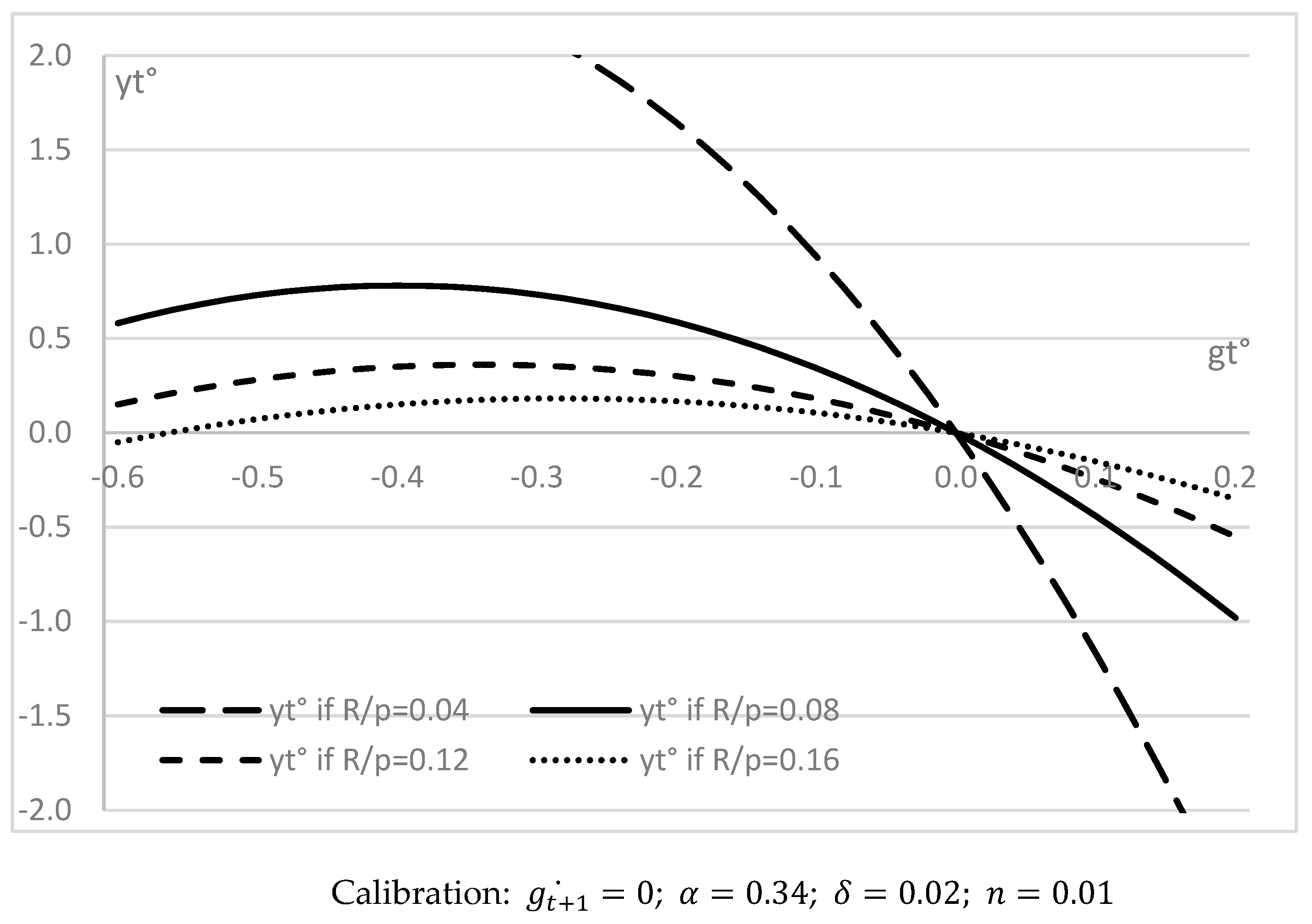
Therefore, Equations (17) and (19) show that even if public consumption expenditures benefit private consumption and contribute to private well-being, they harm global economic activity. Indeed, using also Equation (24), we obtain

$${\displaystyle \frac{\partial y_t}{\partial g_t^C}}=-{\displaystyle \frac{\left[{\left(\frac{{\alpha }_c}{{\alpha }_g}\right)}^{\theta }\frac{\theta \left(1+\phi \right)}{\left(1-\theta \right)}-1\right]\frac{R_t}{P_t}}{\left[\left(\frac{R_t}{P_t}+\alpha -\alpha \delta \right)-\alpha \left(1+n\right)\frac{g_{t+1}^c}{g_t^c}\right]}}$$

(21)

Therefore, public consumption expenditure harms all the more economic activity as the preference is higher for private than for public consumption (${\alpha }_c>{\alpha }_g$) [see Figure 1]. Indeed, according to Equation (21), public consumption expenditure could only be beneficial if

• Households’ preference for private consumption is particularly weak in comparison with their high appetence for public expenditure: ${\displaystyle \frac{{\alpha }_c}{{\alpha }_g}}<{\left[{\displaystyle \frac{\left(1-\theta \right)}{\theta \left(1+\phi \right)}}\right]}^{{\displaystyle \frac{1}{\theta }}}~0.51,$ according to our basic calibration.
• The real return on capital is particularly weak: ${\displaystyle \frac{R_t}{P_t}}<\alpha \left(\delta +n\right)+\alpha \left(1+n\right)\left({\displaystyle \frac{g_{t+1}^c}{g_t^c}}-1\right)~0.01$, according to our basic calibration.

However, these conditions are empirically very weakly plausible, and therefore, public consumption expenditure is mainly detrimental to economic activity. On the contrary, public investment expenditure appears beneficial to economic activity. Indeed, using Equation (22), we obtain

$${\displaystyle \frac{\partial y_t}{\partial g_t^I}}>1 if:g_t^I<{\displaystyle \frac{\alpha \left(1+n\right)}{\left[\alpha \left(1-\delta \right)-\left(1+{\left(\frac{{\alpha }_g}{{\alpha }_c}\right)}^{\theta }\right)\frac{\left(\theta -1\right)}{\left(1+\phi \theta \right)}\frac{R_t}{P_t}\right]}}{g}_{t+1}^I$$

(22)

Therefore, according to Equation (20), our model shows that public investment expenditure decreases private consumption per head. However, according to Equation (18), public investment expenditure also increases income per head provided ${\displaystyle \frac{R_t}{P_t}}>\alpha \left(\delta +n\right)$. Moreover, according to Equation (22), the budget multiplier for public investment expenditure is even higher than one, provided public investment expenditure is sufficiently limited: ($g_t^I<0.87g_{t+1}^I$) according to the basic calibration of our model [see Figure 1]. Therefore, our modeling conforms with the economic literature (see Section 2), distinguishing between public consumption expenditure, which could be harmful, and public investment expenditure, which would be mainly growth-enhancing.

Furthermore, Equations (17) to (20) imply the following level of economic growth, which is identical in the case of growth of public consumption ($\dot{g_t^C}$) or public investment ($\dot{g_t^I}$) expenditure per head:

$$\dot{y_t}=\dot{g_t}-{\displaystyle \frac{\alpha \left(1+\dot{g_t}\right)\left[\left(1+\dot{\frac{R_t}{P_t}}\right)\left(1+n\right)\dot{k_t}+\dot{\frac{R_t}{P_t}}\left(\delta +n\right)-\left(1+n\right)\dot{k_{t+1}}\right]}{\left[\left(1+\dot{\frac{R_t}{P_t}}\right)\frac{R_{t-1}}{P_{t-1}}-\alpha \left(1+n\right)\left(1+\dot{k_{t+1}}\right)+\alpha \left(1-\delta \right)\right]}}$$

(23)

$$\dot{c_t}=\dot{g_t^C}=\dot{g_t^I}=\dot{k_t}$$

(24)

Therefore, public consumption expenditure, public investment expenditure, capital stock, and private consumption per head all increase at the same rate according to Equation (24). As in Afonso and Tovar-Valles (2011), the capital stock positively affects the real GDP per head. Increasing productive ($\dot{g_t^I}$) or even unproductive ($\dot{g_t^c}$) public spending is beneficial to improve the growth of private consumption, and the capital stock (k) strongly positively impacts economic growth [see Equations (23) and (24)]. Nevertheless, according to Equation (23), economic growth can be higher or lower than this common average growth rate of economic variables per head. Indeed:

$${\displaystyle \frac{\partial \dot{y_t}}{\partial \dot{g_t}}}={\displaystyle \frac{\left(1+\dot{\frac{R_t}{P_t}}\right)\left[\frac{R_{t-1}}{P_{t-1}}-\alpha \left(1+\delta +2n\right)-2\alpha \left(1+n\right)\dot{g_t}\right]}{\left[\left(1+\dot{\frac{R_t}{P_t}}\right)\frac{R_{t-1}}{P_{t-1}}-\alpha \left(1+n\right)\left(1+\dot{g_{t+1}}\right)+\alpha \left(1-\delta \right)\right]}}$$

(25)

Therefore, the effect of the variation of investment or consumption public spending per head on economic growth is ambiguous. The economic literature has often underlined a U-shaped relationship between public expenditure and economic activity (see Section 2). However, the contribution of our paper is to show that this relation could also exist between variations of public expenditure and economic growth rates. Indeed, according to Equation (23):

• If $\dot{g_{t+1}}>{\displaystyle \frac{1}{\alpha \left(1+n\right)}}\left(1+\dot{{\displaystyle \frac{R_t}{P_t}}}\right){\displaystyle \frac{R_{t-1}}{P_{t-1}}}-{\displaystyle \frac{\left(\delta +n\right)}{\left(1+n\right)}}$ 

  ○

  Public expenditure is harmful if $\dot{g_t}<{\displaystyle \frac{1}{2\alpha \left(1+n\right)}}\left({\displaystyle \frac{R_{t-1}}{P_{t-1}}}\right)-{\displaystyle \frac{\left(1+\delta +2n\right)}{2\left(1+n\right)}}$

  ○

  Public expenditure is beneficial if $\dot{g_t}>{\displaystyle \frac{1}{2\alpha \left(1+n\right)}}\left({\displaystyle \frac{R_{t-1}}{P_{t-1}}}\right)-{\displaystyle \frac{\left(1+\delta +2n\right)}{2\left(1+n\right)}}$

However, this situation is highly improbable, as according to our basic calibration, the future anticipated increase in public expenditure should be above ($\dot{g_{t+1}}=20.33\%)$ if ($\dot{{\displaystyle \frac{R_t}{P_t}}}=0$). More precisely, the increase in public expenditure could only be beneficial for developing countries, during the limited period of catch-up where the increase in public expenditure per head is very strong in conformity with their development process.

• If $\dot{g_{t+1}}<{\displaystyle \frac{1}{\alpha \left(1+n\right)}}\left(1+\dot{{\displaystyle \frac{R_t}{P_t}}}\right){\displaystyle \frac{R_{t-1}}{P_{t-1}}}-{\displaystyle \frac{\left(\delta +n\right)}{\left(1+n\right)}}$ 

  ○

  Public expenditure is harmful if $\dot{g_t}>{\displaystyle \frac{1}{2\alpha \left(1+n\right)}}\left({\displaystyle \frac{R_{t-1}}{P_{t-1}}}\right)-{\displaystyle \frac{\left(1+\delta +2n\right)}{2\left(1+n\right)}}$

  ○

  Public expenditure is beneficial if $\dot{g_t}<{\displaystyle \frac{1}{2\alpha \left(1+n\right)}}\left({\displaystyle \frac{R_{t-1}}{P_{t-1}}}\right)-{\displaystyle \frac{\left(1+\delta +2n\right)}{2\left(1+n\right)}}$

Therefore, the optimal variation of public expenditure per head depends on capital returns, the depreciation rate of capital, the population growth rate, and the capital share in the production function (see below). However, according to our basic calibration, public expenditure should decrease, for example, by about (−0.4%) to allow a maximal economic growth of (0.78%) if (R/p = 0.08) [see Figure 2].

Moreover, we can study the sensitivity analysis of the robustness of our results to the calibration of the parameters of our model. According to Equation (21), provided [${\displaystyle \frac{R_t}{P_t}}>\alpha \left(n+\delta \right)$], economic growth is higher if the increase of the future anticipated capital per head is higher than the increase of the current capital per head ($\dot{k_t}<\dot{k_{t+1}}$), or if capital returns decrease ($\dot{R_t/p_t}$ < 0). Nevertheless, the influence of the various parameters of our model on economic growth depends on these positive or negative variations of capital and public spending per head. Therefore, our parameters mainly influence the absolute level of revenue or consumption per head.

Public investment expenditure increases income per head but decreases private consumption per head, whereas public consumption expenditure decreases income per head but increases private consumption per head. Nevertheless, according to Equations (17) to (20), public consumption expenditure is less detrimental to economic growth if households’ preferences for public services (${\displaystyle \frac{{\alpha }_g}{{\alpha }_c}}$) are high; however, private consumption is then more limited. Indeed, suppose the preference for public services is high. In that case, a high level of public consumption expenditure provides the same utility to households as a weaker level of private consumption in Equation (1). A high household preference for public services also reduces the beneficial effect of public investment expenditure on economic growth.

Public investment expenditure increases income per head but decreases consumption per head. Then, a higher elasticity of intertemporal substitution (θ) or a higher inverse of the Frisch elasticity of labor supply (φ) is beneficial. Indeed, the increase in income per head is accentuated, whereas the decrease in private consumption is reduced. The increase in income head is also accentuated if the capital share in the production function (α), the capital depreciation rate (δ), or the population growth rate (n) is high, whereas the effect of the real return on capital (R/p) is more ambiguous.

On the contrary, public consumption expenditure decreases income per head but increases consumption per head. Then, a higher elasticity of intertemporal substitution (θ) accentuates the decrease in revenue per head, as well as the increase in private consumption. A higher inverse of the Frisch elasticity of labor supply (φ) worsens the decrease in income per head. A higher capital share in the production function (α), capital depreciation rate (δ), or population growth rate (n) also worsens the decrease in income per head. In contrast, the effect of the real return on capital (R/p) is more ambiguous.

The economic literature often assimilates the study of the consequences of the size of the government on economic growth to the analysis of the level of public expenditure. However, beyond this analysis present in Afonso and Tovar-Valles (2011) for example, our theoretical model also allows us to study the effect of various taxation rates, on the side of fiscal resources.

4.2. Fiscal Resources and Economic Growth

Regarding fiscal resources, taxation reduces the incentive to produce, production realized or labor supplied. However, taxation also increases the production of efficient public services and the productivity of production factors. Instead of distinguishing between distortionary (proportional to output, affecting investment choices) and non-distortionary (lump-sum) taxation, we consider three different kinds of taxation rates: on consumption, labor, and capital. In our model, consumption taxation rates affect capital, private consumption, and economic growth rates. Indeed, Equation (A16) in Appendix A implies

$$\dot{c_t}=\dot{k_t}={\left[{\displaystyle \frac{\beta \left(1+{\tau }_{t-1}^c\right)}{\left(1+{\tau }_{t-1}^c(1+\dot{{\tau }_t^c})\right)}}\right]}^{\theta }-1$$

(26)

$${\displaystyle \frac{\partial \dot{c_t}}{\partial \dot{{\tau }_t^c}}}=-{\displaystyle \frac{\theta {\tau }_{t-1}^c{\beta }^{\theta }{\left(1+{\tau }_{t-1}^c\right)}^{\theta }}{{\left(1+{\tau }_{t-1}^c\left(1+\dot{{\tau }_t^c}\right)\right)}^{\theta +1}}}<0$$

(27)

$${\displaystyle \frac{\partial \dot{c_t}}{\partial {\tau }_{t-1}^c}}=-{\displaystyle \frac{\theta {\beta }^{\theta }{\left(1+{\tau }_{t-1}^c\right)}^{\theta -1}\dot{{\tau }_t^c}}{{\left(1+{\tau }_{t-1}^c\left(1+\dot{{\tau }_t^c}\right)\right)}^{\theta +1}}}$$

(28)

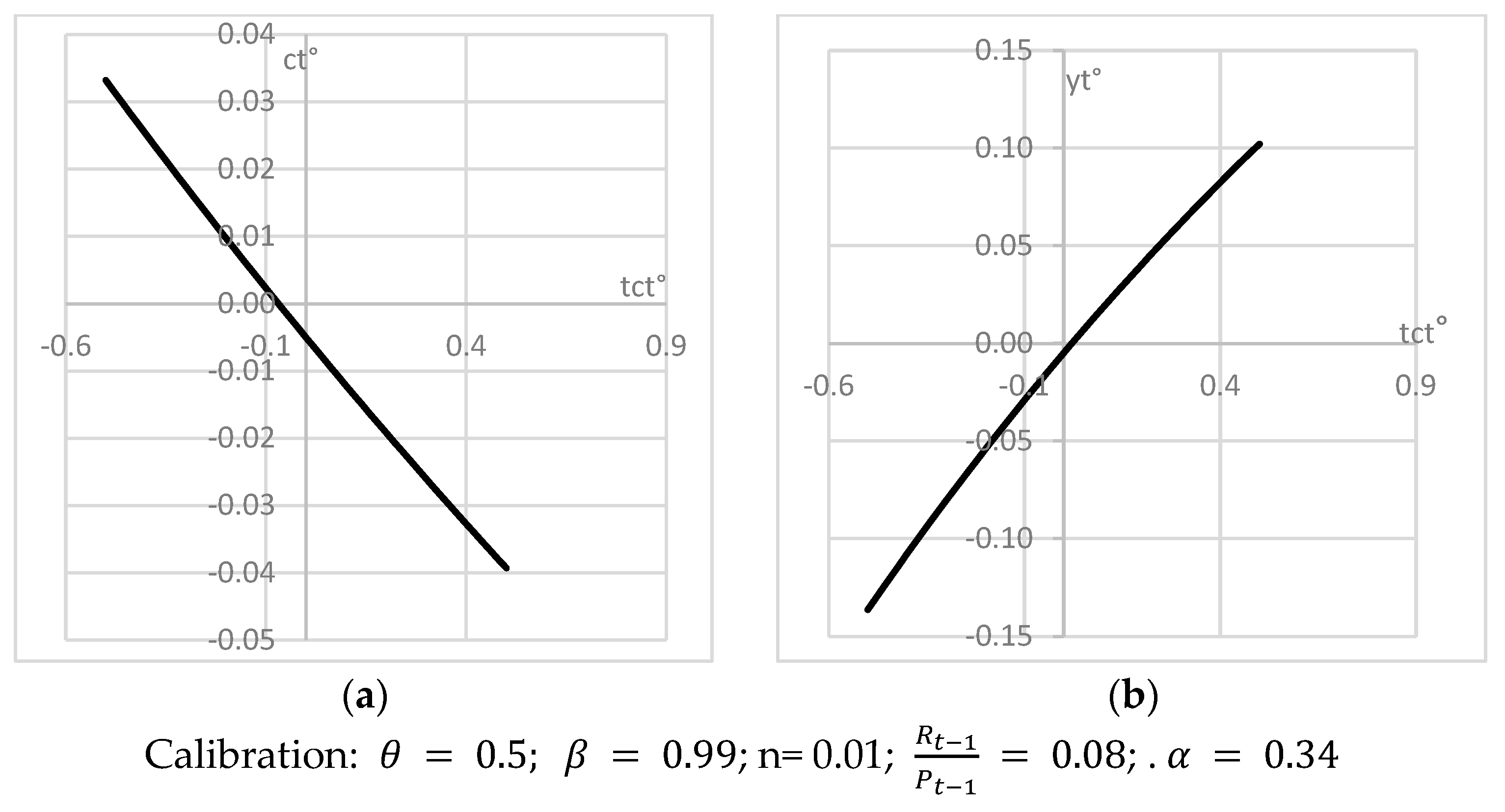
Therefore, according to Equations (27) and (28), a high consumption taxation rate harms private consumption growth if this tax rate increases, but it is beneficial if it decreases. An increase in the consumption taxation rate is always harmful to private consumption growth, whereas a decrease is always helpful, whatever the absolute level of the consumption taxation rate. The relation would be linear, but consumption taxation rate variations would only marginally modify private consumption growth [see Figure 3].

On the contrary, regarding economic growth, Equation (A20) in Appendix A implies

$$\begin{gathered} \dot{y_t}={\left[{\displaystyle \frac{\beta \left(1+{\tau }_{t-1}^c\right)}{\left(1+{\tau }_{t-1}^c\left(1+\dot{{\tau }_t^c}\right)\right)}}\right]}^{\theta }-{\displaystyle \frac{\alpha \left(1+n\right)}{\frac{R_{t-1}}{P_{t-1}}}}{\left[{\displaystyle \frac{\beta \left(1+{\tau }_{t-1}^c\right)}{\left(1+{\tau }_{t-1}^c\left(1+\dot{{\tau }_t^c}\right)\right)}}\right]}^{2\theta }-1 \\ \hspace{1em}\hspace{1em}\hspace{1em}\hspace{1em}+{\displaystyle \frac{\alpha \left(1+n\right)}{\frac{R_{t-1}}{P_{t-1}}}}{\left[{\displaystyle \frac{{\beta }^2\left(1+{\tau }_{t-1}^c\right)}{\left(1+{\tau }_{t-1}^c\left(1+\dot{{\tau }_t^c}\right)\left(1+\dot{{\tau }_{t+1}^c}\right)\right)}}\right]}^{\theta } \end{gathered}$$

(29)

Therefore, even if it is detrimental to private consumption, increasing the current consumption taxation rate ($\dot{{\tau }_t^c}>0$) seems beneficial to economic growth [see Figure 3]. Therefore, increasing the share of fiscal resources collected by way of consumption taxes, in comparison with taxing capital or labor, could benefit global economic growth.

Moreover, in the short run as in the long run, according to Equations (26) and (29), private consumption and global economic activity growth increase with the time discount factor (β), but they decrease with the elasticity of intertemporal substitution (θ) [$\dot{c}=\dot{y}={\beta }^{\theta }-1$]. Indeed, the higher the time discount factor, the higher the preference for future consumption and sparing, and the higher the capital growth rate per head. Furthermore, in the short run, three factors can modify economic growth. According to Equation (29), the real return on capital (R/p), or the capital share in the production function (α), only marginally modifies the economic growth rate depending on the variation of the consumption taxation rate. According to Equation (29), a third factor influencing economic growth in the short run is population growth (n). However, demographic growth also only marginally modifies economic growth depending on the variation of the consumption taxation rate. Moreover, these variables do not affect private consumption or economic growth in the long run.

In this context, economic authorities could be tempted to arbitrate between increasing private consumption (${\alpha }_c$) and global economic growth (${\alpha }_y$). Therefore, using Equations (26) and (29), we obtain the following average well-being in Equation (30):

$$\begin{gathered} {\alpha }_c\dot{c_t}+{\alpha }_y\dot{y_t}=({\alpha }_c+{\alpha }_y)\left\{{\left[{\displaystyle \frac{\beta \left(1+{\tau }_{t-1}^c\right)}{\left(1+{\tau }_{t-1}^c\left(1+\dot{{\tau }_t^c}\right)\right)}}\right]}^{\theta }-1\right\} \\ \hspace{1em}\hspace{1em}\hspace{1em}\hspace{1em}\hspace{1em} \hspace{1em}\hspace{1em}\hspace{1em}+{\alpha }_y{\displaystyle \frac{\alpha \left(1+n\right){\beta }^{2\theta }}{\frac{R_{t-1}}{P_{t-1}}}}\{{\left[{\displaystyle \frac{\left(1+{\tau }_{t-1}^c\right)}{\left(1+{\tau }_{t-1}^c\left(1+\dot{{\tau }_t^c}\right)\left(1+\dot{{\tau }_{t+1}^c}\right)\right)}}\right]}^{\theta }-{\left[{\displaystyle \frac{\left(1+{\tau }_{t-1}^c\right)}{\left(1+{\tau }_{t-1}^c\left(1+\dot{{\tau }_t^c}\right)\right)}}\right]}^{2\theta }\} \end{gathered}$$

(30)

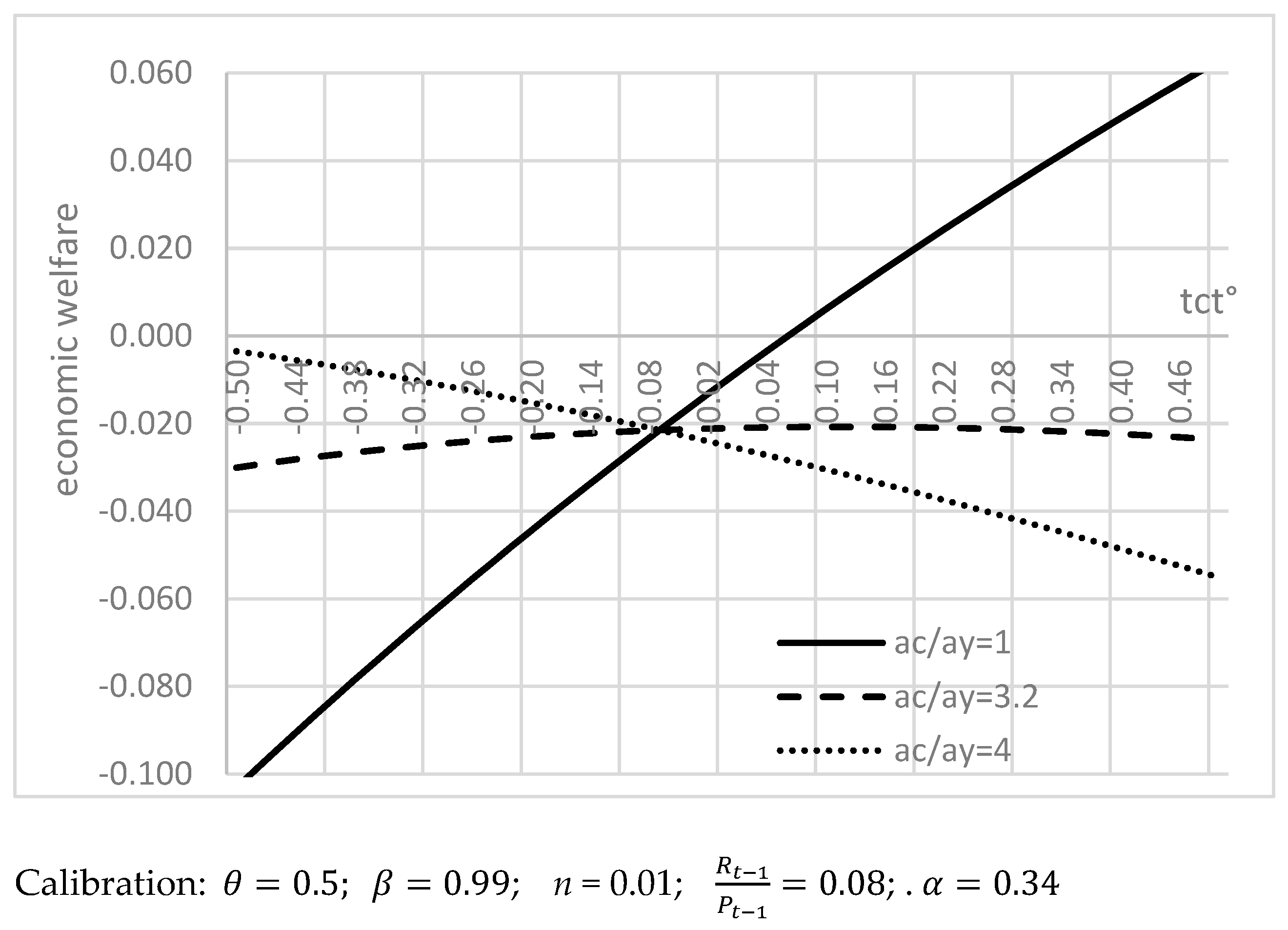
Therefore, as mentioned above, increasing the consumption taxation rate could benefit global economic growth, whereas moderating the consumption taxation rate could benefit private consumption. So, it is only in the intermediate case of an arbitrage slightly in favor of private consumption ($3<{\displaystyle \frac{{\alpha }_c}{{\alpha }_y}}<3.5$) that there could be an inverted U-shaped relation between the increase of the consumption taxation rate and an indicator of economic well-being, with a maximal taxation rate to collect the optimal level of fiscal resources [see Figure 4].

Furthermore, in these conditions, if the government’s goal is to target an equilibrium budget, a higher consumption taxation rate should be compensated with a decrease in the labor or capital taxation rate. Therefore, according to Equation (A22) in Appendix A, these variations should be such as

$$\begin{gathered} \left[\alpha {\tau }_{t-1}^k\dot{{\tau }_t^k}+\left(1-\alpha \right){\tau }_{t-1}^l\dot{{\tau }_t^l}\right]\hspace{1em}\hspace{1em}\hspace{1em}\hspace{1em}\hspace{1em}\hspace{1em}\hspace{1em}\hspace{1em}\hspace{1em}\hspace{1em} \\ ={\displaystyle \frac{{\tau }_{t-1}^c\dot{{\tau }_t^c}}{\left(1+{\tau }_{t-1}^c\right)\left[\frac{\alpha \left(1+n\right){\beta }^{\theta }{\left(1+{\tau }_{t-1}^c\left(1+\dot{{\tau }_t^c}\right)\right)}^{\theta }}{{\left(1+{\tau }_{t-1}^c\left(1+\dot{{\tau }_t^c}\right)\left(1+\dot{{\tau }_{t+1}^c}\right)\right)}^{\theta }}-\frac{\alpha \left(1+n\right){\beta }^{\theta }{\left(1+{\tau }_{t-1}^c\right)}^{\theta }}{{\left(1+{\tau }_{t-1}^c\left(1+\dot{{\tau }_t^c}\right)\right)}^{\theta }}+\frac{R_{t-1}}{P_{t-1}}\right]}} \\ \hspace{1em}\hspace{1em}\hspace{1em}\hspace{1em} \hspace{1em}\hspace{1em}\hspace{1em}\hspace{1em}\hspace{1em}\hspace{1em}\hspace{1em}\hspace{1em}\hspace{1em}\hspace{1em}\{\alpha \left(1+n\right){\beta }^{\theta }{\left[{\displaystyle \frac{\left(1+{\tau }_{t-1}^c\right)}{\left(1+{\tau }_{t-1}^c\left(1+\dot{{\tau }_t^c}\right)\right)}}\right]}^{\theta }+{\displaystyle \frac{\left(1+{\tau }_{t-1}^c\left(1+\dot{{\tau }_t^c}\right)\right)}{{\tau }_{t-1}^c\dot{{\tau }_t^c}}}\left[\alpha {\tau }_{t-1}^k+\left(1-\alpha \right){\tau }_{t-1}^l\right]{\displaystyle \frac{R_{t-1}}{P_{t-1}}} \\ \hspace{1em}\hspace{1em}\hspace{1em}\hspace{1em}\hspace{1em}\hspace{1em}\hspace{1em}\hspace{1em}\hspace{1em}\hspace{1em}\hspace{1em}-\alpha \left(1-\delta \right)-{\displaystyle \frac{R_{t-1}}{P_{t-1}}}\}-\left[\alpha {\tau }_{t-1}^k+\left(1-\alpha \right){\tau }_{t-1}^l\right] \end{gathered}$$

(31)

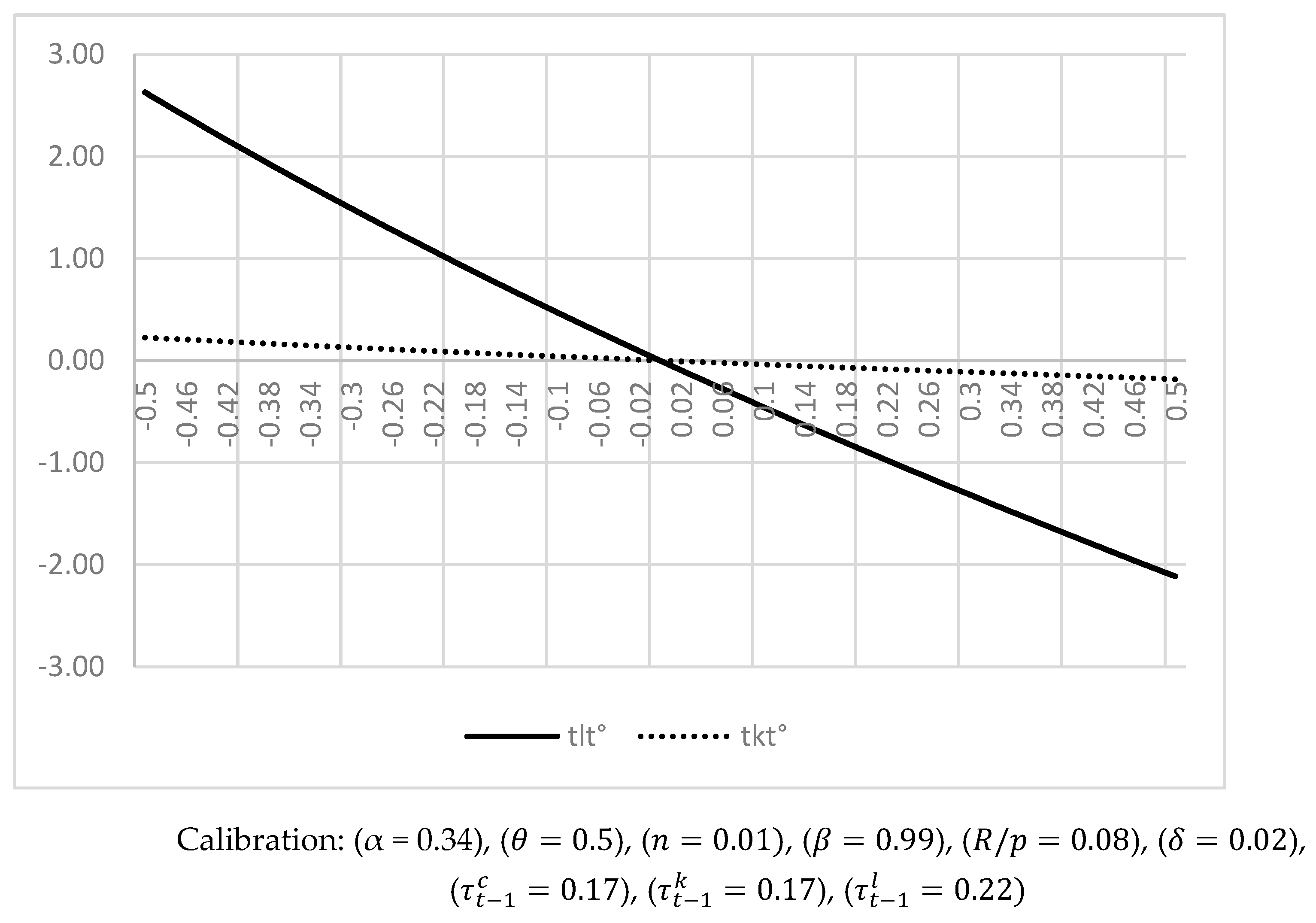
Therefore, to compensate for a higher (smaller) consumption taxation rate, beneficial to economic growth, and to equilibrate the budget balance, the decrease (increase) in the labor taxation rate could be more accentuated than the decrease (increase) in the capital taxation rate [see Figure 5]. Indeed, according to the parameter (α), the labor share in the production function is about twice higher than the capital share in the production function. The absolute levels of the capital or labor taxation rates have no effect in the long run, as Equation (30) is always verified. However, if the consumption taxation rate (${\tau }_{t-1}^c$) is higher, compensatory variations in the labor or capital taxation rates are both more accentuated. Moreover, if the labor taxation rate (${\tau }_{t-1}^l$) is higher, variations in the labor taxation rate are strongly accentuated, whereas variations in the capital taxation rate are much more moderate. On the contrary, if the capital taxation rate (${\tau }_{t-1}^k$) is higher, variations in the capital taxation rate are only very slightly accentuated, whereas variations in the labor taxation rate are significantly more moderate.

Furthermore, according to Equation (31), optimal variations in the labor or capital taxation rates also depend on variations of other variables. Indeed, if the capital share in the production function (α) increases, variations in the labor taxation rates should be reduced, whereas variations in the capital taxation rates should be accentuated. Moreover, if the real capital returns (R/p) or if the intertemporal elasticity of substitution (θ) increase, variations in the labor and capital taxation rates should be accentuated. On the contrary, if the capital depreciation rate (δ), the population growth rate (n), or the time discount factor (β) increases, variations in the labor or capital taxation rates should be mitigated. Therefore, a higher consumption taxation rate is likely to favor a higher global economic growth rate. The capital and mainly the labor taxation rate could then simultaneously be reduced without consequences on global fiscal resources and the budget. Nevertheless, the intensity of the decrease allowed in capital or labor taxation rates depends on other economic variables.

4.3. Empirical Observations

The current paper is theoretical, and we leave for future research the empirical verification by econometrical methods of our hypotheses. However, a first look at empirical data show that these theoretical hypotheses could be verified. For the European Union, these data come from the AMECO database for global economic growth rates, final consumption expenditure, and gross fixed capital formation of the governments in 2024. Data come from the website of the European Commission for the year 2022 (last available data) for the implicit tax rate on consumption.

In 2024, the average annual GDP growth rate was 1.12% in the European Union, whereas for the governments, on average, final consumption expenditure represented 21.5% of GDP and gross fixed capital formation 3.7% of GDP at current market prices. However, in conformity with our hypotheses, we can note that economic growth was higher in a group of countries where the share of public investment expenditure was high. Indeed, public gross fixed capital formation and economic growth were both higher than the European average in Croatia (respectively, 5.7% and 3.4%), Romania (5.7% and 1.91%), Slovenia (5.2% and 1.5%), Poland (5% and 2.96%) or in Greece (4.9% and 2.28%). On the contrary, public gross fixed capital formation and economic growth were both weaker than the European average in the Netherlands (respectively, 3.1% and 0.63%), Germany (3% and 0.01%), or Ireland (2.5% and −0.18%). Moreover, economic growth was also higher in a group of countries where public consumption expenditure was weak. Indeed, the share of public final consumption expenditure in GDP was weak in a group of countries where economic growth was higher than the European average: Portugal (respectively 16.8% and 1.93%), Malta (17.2% and 5%), Lithuania (18.1% and 2.43%), Cyprus (18.6% and 3.29%), Romania (18.8% and 1.91%), Greece (19.2% and 2.28%), Spain (19.4% and 2.91%), or in Bulgaria (19.6% and 2.32%). On the contrary, the share of public final consumption expenditure in GDP was high in a group of countries where economic growth was weaker than the European average: in Sweden (respectively, 26.6% and 0.9%), Finland (26.4% and −0.1%), or in the Netherlands (25.1% and 0.63%).

Furthermore, in 2024, the adjusted wage share in labor costs represented 62.9% of the GDP on average in the European Union. However, in conformity with our hypothesis, we can note that increasing public spending could mainly be beneficial in countries where capitalization (share of capital in the production function) is weak. Indeed, the wage share in labor costs was higher in a group of countries where public gross fixed capital formation or final consumption expenditure was higher than the European average: in Slovenia (respectively, 74.3%, 5.2%, and 20.9%), Latvia (73.8%, 5.3%, and 22.5%), France (66.8%, 4.3%, and 24.3%), Croatia (66.1%, 5.7%, and 22.6%), or in Estonia (64.7%, 7.3%, and 21.1%). On the contrary, the wage share in labor costs and public gross fixed capital formation or final consumption expenditure were all weaker than the European average in Ireland (respectively, 36%, 2.5%, and 13%), Malta (50.3%, 4.1%, and 17.2%), Slovakia (54%, 3.7%, and 20.8%), or in Cyprus (56.5%, 2.9%, and 18.6%).

Moreover, in 2024, the average GDP growth rate was 1.12% in the European Union, whereas the implicit tax rate on consumption was 17.2%. However, in conformity with our hypothesis, we can note that economic growth was higher in a group of countries where consumption taxes were high. Indeed, implicit consumption taxes and economic growth were both higher than the European average in Denmark (respectively, 23.4% and 1.94%), Hungary (22.9% and 1.48%), Croatia (21.3% and 3.4%), Greece (20.2% and 2.28%), Slovenia (19.6% and 1.5%), Bulgaria (19% and 2.32%), Poland (18% and 2.96%), Lithuania (17.6% and 2.43%), Cyprus (17.4% and 3.29%) or in Malta (17.3% and 5%). On the contrary, implicit consumption taxes and economic growth were both weaker than the European average in Germany (respectively, 16.0% and 0.01%) or in Italy (16% and 0.67%).

5. Conclusions

Our paper aims to shed light on the potential effect of fiscal policy on economic growth: the determinants of a positive or negative impact of public expenditure, and the various ways to collect the necessary fiscal resources. Regarding public spending, we show that public consumption expenditure usually harms global economic growth, and all the more as real capital returns are high, and as the preference of the representative consumer is much higher for private consumption than for public consumption. On the contrary, even if consumption decreases per head, public investment expenditure appears to benefit economic activity: it can increase income per head, provided real returns on capital are not too small. Investment public spending is then all the more beneficial as the capital share in the production function, the capital depreciation rate, and the population growth rate are high. Moreover, we can theoretically underline the existence of an inverted U-shaped relation between the variation of public expenditure and economic growth. An increase in public spending would be beneficial to economic growth only up to a maximal variation, which positively depends on real capital returns. Increasing public spending could also mainly be beneficial in countries where the capitalization (share of capital in the production function) is weak.

As a practical implication of the paper for policymakers, obviously, economic policies should favor the increase in public investment rather than public consumption expenditure. An excessive increase in public spending could be detrimental beyond a given level, especially for countries where the capital share in the production function is high, or where the preference for public services is weak. Regarding fiscal resources, we show that policymakers should favor an increase in the share of fiscal resources collected through consumption taxes. Indeed, such an increase could be beneficial to global economic growth, even if it is detrimental to private consumption. Then, in parallel to the increase in consumption taxes, it could be possible to reduce capital taxation rates, and mainly to strongly reduce labor taxation rates.

Our paper was only interested in the effect of public expenditure on economic growth. However, there are many other implications of public spending, beyond the scope of the current paper: social equity and redistribution, quality of life and well-being including environmental considerations and security at the national and international level, etc. Public spending is not the best way to increase economic growth; often, it is not appropriate in terms of efficiency. However, public spending is usually justified to correct market failures, inefficiency in the private production of some public services, or for justice or equity considerations.

The extension of the current paper would be to continue to study the consequences of the size of the public sector on economic growth. Theoretically, my future research direction is to try to evaluate the optimal size of public spending in various countries, according to the characteristics and the macroeconomic parameters of these countries. Many econometrical studies have suggested such optimal sizes. However, a natural future prolongation of the current theoretical study would be to link this optimal size to the macroeconomic parameters of the countries.

References

1. Afonso, A., & Furceri, D. (2010). Government size, composition, volatility and economic growth. European Journal of Political Economy, 26(4), 517–532. [Google Scholar] [CrossRef]
2. Afonso, A., & Tovar-Valles, J. (2011). Economic performance and government size. Working Paper Series 1399. European Central Bank. [Google Scholar]
3. Asimakopoulos, S., & Karavias, Y. (2016). The impact of government size on economic growth: A threshold analysis. Economic Letters, 139. [Google Scholar] [CrossRef]
4. Bergh, A., & Henrekson, M. (2011). Government size and growth: A survey and interpretation of the evidence. Journal of Economic Surveys, 25(5), 872–897. [Google Scholar] [CrossRef]
5. Bergh, A., & Karlsson, M. (2010). Government size and growth: Accounting for economic freedom and globalization. Public Choice, 142(1–2), 195–213. [Google Scholar] [CrossRef]
6. Carvalho, V. M., & Martins, M. M. F. (2011). Macroeconomic effects of fiscal consolidations in a DSGE model for the Euro Area: Does composition matter? FEP Working Papers 421. Universidade do Porto, Facultade de Economia do Porto. [Google Scholar]
7. Cenc, H. (2022). Government expenditure and economic growth in Euro area countries. Naše gospodarstvo/Our Economy, 68(2), 19–27. [Google Scholar] [CrossRef]
8. Cepparulo, A., & Mourre, G. (2020). How & how much? The growth-friendliness of public spending through the lens. In European economy. Discussion Paper 132. European Commission. [Google Scholar]
9. Chobanov, D., & Mladenova, A. (2009). What is the optimum size of government. Institute for Market Economics. [Google Scholar]
10. Christie, T. (2014). The effect of government spending on economic growth: Testing the non-linear hypothesis. Bulletin of Economic Research, 66(2), 183–204. [Google Scholar] [CrossRef]
11. Coayla, E. (2021). The optimal size of government and the Armey curve: A review of empirical evidence. Applied Economics Journal, 28(1), 121–137. [Google Scholar]
12. European Commission. (2024). Annual report on taxation; review of taxation policies in EU member states. Luxembourg. [Google Scholar]
13. Fall, F., & Fournier, J. M. (2015). Macroeconomic uncertainties, prudent debt targets and fiscal rules. OECD Economics Department Working Papers 1230. OECD Economics Department. [Google Scholar]
14. Forte, F., & Magazzino, C. (2011). Optimal size government and economic Growth in EU countries. Economia Politica, 28(3). [Google Scholar]
15. Fournier, J.-M., & Johansson, A. (2016). The effect of the size and the mix of public spending on growth and inequality. OECD Economics Department Working Paper 1344. OECD Economics Department. [Google Scholar]
16. Fölster, S., & Henrekson, M. (2001). Growth effects of government expenditure and taxation in rich countries. European Economic Review, 45(8), 1501–1520. [Google Scholar] [CrossRef]
17. Johansson, A., Heady, C., Arnold, J. M., Brys, B., & Vartia, L. (2008). Taxation and economic growth. OECD Economics Department Working Papers 620. OECD Economics Department. [Google Scholar]
18. Kutasi, G., & Marton, A. (2020). The long term impact of public expenditures on GDP-growth. Society and Economy, 42(4), 403–419. [Google Scholar] [CrossRef]
19. Martins, S., & Veiga, F. J. (2014). Government size, composition of public expenditure, and economic development. International Tax and Public Finance, 21, 578–597. [Google Scholar] [CrossRef]
20. Mitu, N. E., & Stanciu, C. V. (2023). Public sector performance and public sector efficiency: An analysis for CEE countries. Eastern European Economics, 61(6), 700–722. [Google Scholar] [CrossRef]
21. Myles, G. D. (2009). Economic growth and the role of taxation–Theory. OECD Economics Department Working Papers 713. OECD Economics Department. [Google Scholar]
22. Negri, C., & Dinca, G. (2023). Public sector’s efficiency as a reflection of governance quality: A European Union study. PLOS ONE, 18(9). [Google Scholar] [CrossRef] [PubMed]
23. Romero-Avila, D., & Strauch, R. (2008). Public finances and long-term growth in Europe: Evidence from a panel data analysis. European Journal of Political Economy, 24(1), 172–191. [Google Scholar] [CrossRef]
24. Scully, G. (1994). What is the optimal size of government in the United States? Policy Report 188. National Center for Policy Analysis. [Google Scholar]
Figure 1. Variation of public expenditure and variation of economic activity. (a) Variation of economic activity according to the variation of public consumption; (b) Variation of economic activity according to the variation of public investment.
Economies 13 00074 g001
Figure 2. Variation of public expenditure per head and economic growth.
Economies 13 00074 g002
Figure 3. Variation of the consumption taxation rate and economic growth: (a) Variation of private consumption according to the variation of the consumption taxation rate; (b) Variation of economic activity according to the variation of the consumption taxation rate.
Economies 13 00074 g003
Figure 4. Variation of the consumption taxation rate and economic welfare.
Economies 13 00074 g004
Figure 5. Optimal labor and capital taxation rates.
Economies 13 00074 g005
Disclaimer/Publisher’s Note: The statements, opinions and data contained in all publications are solely those of the individual author(s) and contributor(s) and not of MDPI and/or the editor(s). MDPI and/or the editor(s) disclaim responsibility for any injury to people or property resulting from any ideas, methods, instructions or products referred to in the content.