Abstract
This research demonstrates the potential of machine learning for revealing the fiscal effects of the Recovery and Resilience Facility (RRF) in the European Union. It focuses on the use of a hybrid approach, based on traditional econometric methods combined with advanced data machine learning techniques. For this purpose, the following were applied: a panel data model with fixed effects, difference-in-differences analysis, correlation analysis, and machine learning, specifically, random forest regression, for the period of 2020–2024, including indicators from all 27 EU member states. The results of the conducted tests establish the effectiveness of the Recovery and Resilience Facility for fiscal stabilization, but also its high vulnerability to specific economic conditions in the individual member states. The complex relationships between the amount of funds received and the fiscal outcomes, which classical models fail to capture, were derived. A positive stabilizing effect on the indebtedness of countries with a clearly expressed imbalance in the public debt-to-gross domestic product ratio was demonstrated.
1. Introduction
The Recovery and Resilience Facility (RRF) is historically the largest-scale and most innovative instrument for the economic recovery of the EU, introduced in response to the COVID-19 pandemic. The innovative governance model radically changes the way the EU works on the economic policies of its member states. It is a key instrument of Next Generation EU, whose aim is to support economic recovery after COVID-19 through coordinated financing in structural reforms. The motivation for the present research is the need to establish whether this unprecedented instrument fulfills its objectives for economic growth and fiscal stability, and to provide recommendations for improving future European policies. At the same time, the results can be informative regarding the enhancement of the effectiveness of subsequent European fiscal instruments. In this regard, the object of this research is the Recovery and Resilience Facility in the EU. The subject of this research is the application of machine learning to data for modeling the impact of the Recovery and Resilience Facility on fiscal indicators.
The main thesis of this study is that the disbursements under the Recovery and Resilience Mechanism have a consistent, statistically significant, and positive effect on the stabilization of the fiscal balance in the EU member states. This is manifested not only in the reduction in the deficit and stabilization of the public debt, but also as a multiplier effect on economic activity, which is stronger in countries with higher GDP per capita and more efficient absorption of funds. The present study focused on testing the following hypotheses:
Hypothesis 1.
The disbursements under the Recovery and Resilience Facility generate a statistically significant and positive multiplier effect on the fiscal balance of EU member states.
Hypothesis 2.
Countries with a higher GDP per capita realize a stronger multiplier effect from the Recovery and Resilience Facility funds due to higher administrative capacity and investment efficiency.
Hypothesis 3.
The COVID-19 pandemic had a negative effect on the fiscal balance, but this effect is partially offset by the Recovery and Resilience Facility funds.
Hypothesis 4.
The effect of the Recovery and Resilience Facility funds on the fiscal balance manifests itself with a delay due to the investment nature of the costs and the time needed to implement the projects.
Hypothesis 5.
The Recovery and Resilience Facility funds have a higher explanatory power for the fiscal balance compared with traditional macroeconomic factors (GDP, inflation, and unemployment).
The aim of this work is to assess the multiplier effect of the Recovery and Resilience Facility on EU countries. The tasks on which the current work focuses are as follows:
First. To outline the theoretical framework of the Recovery and Resilience Facility.
Second. To analyze existing research and practices.
Third. To apply quantitative methods for assessing the fiscal effects.
Fourth. To assess the multiplier effect of the European Union’s Recovery and Resilience Facility.
Fifth. To propose recommendations for optimizing EU instruments and fiscal policies.
2. Theoretical Framework for the European Union and the EU Recovery and Resilience Facility
The European Union has always sought integration through economic and political mechanisms, with the focus undergoing significant change in the different stages of its functioning. The key objectives of the Union evolve over time: from deepening common policies, regional development, and macroeconomic coordination, through the creation of a common currency, institutional reforms, and expansion of cooperation, to achieving social cohesion, scientific and technological progress, sustainable development, and well-being. Throughout its history, the EU has always striven for integrity and minimizing imbalances in individual countries to achieve unity among the states. In the modern era, the key aspirations of the EU are achieving strategic autonomy, digital transformation, and the green transition. One of the most important innovations introduced in the EU in the early 1990s was the creation of a multi-level governance system, applied to the management of operational programs financed by the structural funds (Leonardi & Nanetti, 2011). Years later, the question remains: whether differences in the institutional structures of member states have led to different approaches to effective choice, and how effective the funds directed toward stakeholders have been. In this regard, the context of this study includes the largest EU instrument for achieving solidarity during the global COVID-19 pandemic, convergence between regions, the introduction of institutional innovations, and the green and digital transition: the Recovery and Resilience Facility in the EU. It is an example of a pan-European instrument strengthening economic solidarity and supporting member states in overcoming crises. From a theoretical perspective, it is based on the Keynesian principles of the active role of the state in the economy (Terra et al., 2020). Meanwhile, it corresponds to the Real Business Cycle Theory (Kydland & Prescott, 1982), which examines the negative influence of external shocks on economic equilibrium. Additionally, the concept of asymmetric shocks (Mundell, 1961) explains why the effects of crises manifest differently in individual countries. The creation of the RRF also actively advocates for the theory of institutional evolution (Pierson, 2000) and emphasizes how crises act as a catalyst for introducing institutional innovations. In its essence, the EU instrument can also be viewed as a hybrid instrument—a supranational tool, raising questions about the transfer of resources from the national to the supranational level (Oates, 1999). The governance model of the RRF introduces a new level of multi-level governance and resembles a system where policy creation is shared among different levels of government: local, regional, national, and international, encouraging cooperation and coordination for effective problem solving and decision making (Hooghe & Marks, 2007). It is the combination of common debt, grants, and loans that makes it unique compared with previous EU instruments.
The Recovery and Resilience Facility, the largest financial instrument in the history of the EU, with funds amounting to EUR 672.5 billion, combining grants and loans, is directed toward six strategic priorities. Of these, 46% are grants, and 54% are foreseen for loan resources (European Commission, 2020). The mechanism itself is part of the “Next Generation EU” element (2021–2024) of the European Recovery Plan. The criteria (Nextgeneration, 2025) for the distribution of funds among member states are divided into two groups. The first group (70% of the grants) covers the size of the population; the reciprocal value of GDP per capita; and the average level of unemployment over the last 5 years (2015–2019), compared with the EU average level. The remaining thirty percent of the funds is provided based on the observed loss of real GDP in 2020 and the observed cumulative loss of real GDP for the period of 2020–2021, which was calculated up to 30 June 2022.
The main priority pillars of the mechanism are green transition, digital transformation, smart, sustainable and inclusive growth, social and territorial cohesion, healthcare, economic, social, and institutional resilience, and policies for the next generation (Natea, 2022). All the indicated directions require support for adaptation to the new global paradigms, which vary in degree across different EU countries depending on progress and priorities. For the purpose of applying for the facility, each member state prepares its own Recovery and Resilience Plan, addressing reforms that will lead to economic growth, job creation, strengthening social resilience, and fiscal sustainability. In this regard, this study analyzes data on key indicators related to public finance and traceable socio-economic measures. Historically, the EU has already used similar support and financing instruments: Structural and Cohesion Funds, the European Stability Mechanism, the European Fund for Strategic Investments, and others. Compared with the previous EU instruments, the Recovery and Resilience Facility is a temporary crisis instrument, whereas the Structural and Cohesion Funds are a permanent part of the EU member states’ cohesion policy. Under the RRF, milestones and targets are executed, rather than focusing on budget absorption. Unlike the European Stability Mechanism, which supports Eurozone countries in severe financial difficulties (debt crises), the Recovery and Resilience Facility is a preventive and stimulating instrument for growth and resilience. Its financing is linked to strategic reforms: digitalization, green economy, and social resilience. Compared with the European Fund for Strategic Investments, which aims to stimulate private investments through guarantees and risk taking by the European Investment Bank, the RRF works through direct public financing and establishes a basis for structural reforms and resilience. In practice, the mechanism can be considered the first step toward a de facto fiscal union, which makes it different from previous EU instruments.
Given the above, the RRF in the EU can be considered not merely as another European mechanism, but as a catalyst for institutional changes and the first crisis fund of its kind. It is based on common debt at the European level and combines grants with a significant amount of credits. A key element in its operation is the linking of funds to specific reforms aimed at the green and digital transition of the member states. As a hybrid model between cohesion policy and a crisis stabilization mechanism after the COVID-19 pandemic, it represents a new financial and economic phenomenon in the EU’s integration practice. The success of the mechanism largely depends on the capacity of the countries to plan, implement, manage, and track the results of the actions taken.
3. Review of Research on the Topic
A review of the existing scientific research shows differences in techniques and directions that diverge from the objectives and approach of the current study. A broad base of literature sources was studied, and works with a point of contact to the current paper were synthesized. In this regard, the study by Fabbrini (2024) focused on the new legal technology of European governance introduced by the RRF and its growing proliferation in numerous internal and external EU programs. Since 2021, the legal framework of the RRF has also been applied in a number of other European initiatives, including Re Power EU, the EU Social Climate Fund, the Macro-Financial Assistance Instrument for Ukraine, and others. According to F. Fabbrini, if Next Generation EU (NGEU) is considered transformative for the use of common EU debt, from a legal and governance perspective, the RRF is perhaps one of the main legacies of the EU’s response to the pandemic. In their work, Hodson and Howarth (2023) dispute the unprecedented nature of the mechanism, arguing that it is part of the already familiar EU practice of balanced financial decisions. According to the authors, “Its creation is an example of the EU’s tendency to switch between intergovernmental and supranational modes of lending, as our findings show, as well as the limited impulse to extend or reproduce the EU’s pandemic fund in response to the war in Ukraine”. Zeitlin et al. (2024) analyzed the practical implementation of national plans and defined the RRF as a new type of instrument, “demand-driven and results-based,” which is aimed at overcoming the limitations of past policies intended to encourage national reforms. In their study, they evaluated its practical effectiveness and legitimacy by analyzing the drafting, implementation, and monitoring of National Recovery and Resilience Plans in eight member states. A detailed analysis of the macroeconomic effects of the RRF was also performed by Watzka and Watt (2020). They used the macroeconomic multinational model (NiGEM) to analyze the macroeconomic effects of the mechanism. They showed that the mechanism has the potential to reduce disparities between member states, especially in Southern and Eastern Europe, while also supporting the reduction in debt levels. Their analysis was supplemented by Millard (2025), who used a global model to examine the effects on GDP and fiscal stability. He drew attention to three key channels through which the mechanism can influence the macroeconomy: the risk premium channel, the public investment channel, and the structural reforms channel. He believes that the announcement of a recovery fund can lead to a significant reduction in spreads for many EU countries, increasing their fiscal effect, albeit with a negligible effect on GDP. In their research, Borović et al. (2024) applied a log t-test for the period of 2003–2023 to examine the formation of clusters for productivity and institutional convergence. The results show the existence of multiple stable states, meaning that the EU is vulnerable to external economic shocks. A significantly more in-depth study of the effects of the EU RRF was conducted by Guillamón et al. (2021). They assessed the distribution of funds for the period of 2021–2022, and through regression analysis, they investigated whether other health indicators directly related to the pandemic could also be associated with the amount of funding EU countries would receive during the period. They concluded that criteria such as population, GDP per capita, and unemployment had the greatest influence on determining the grants.
The literature review shows the topicality of the subject but also highlights significant methodological and analytical gaps. The existing studies provide valuable observations but are limited to traditional models that cannot capture the complex non-linear interactions in the data. A large part of the studies focuses on macroeconomic effects without going into detail about their impact on individual policies. This, in turn, limits the possibility of formulating targeted recommendations for political action. At the same time, there is a lack of depth regarding the specific multiplier effects of the mechanism and what the possible long-term prospects are. The present study is distinguished by combining econometric methods with machine learning to investigate fiscal effects, not just macroeconomic ones. The hybrid application aims to demonstrate that machine learning methods can detect interactions between variables that classical models fail to capture. The novelty of the present study lies not in the use of a machine learning algorithm per se, but in its integration into a framework that also includes causal inference techniques. In this way, it shows how ML can be used not to prove, but to identify potential causal models that are validated through econometrics.
The foregoing clearly emphasizes the need for an in-depth analysis of the effects of the EU RRF through the application of a complex set of tools. This stems from the point of contact between the theoretical significance of the mechanism and the practical necessity of optimizing policies and opportunities. This research will attempt to fill the critical gaps in the literature by providing a deeper understanding of the mechanism and practical tools for improving the effectiveness of European policy. In the context of increasing uncertainty and the need for adaptive policy solutions, this type of research is considered not only timely but also strategically necessary for future European development.
4. Methodology
To assess the multiplier effect of the RRF in the EU and derive its fiscal effects, a complex quantitative approach was adopted. The analysis applied a panel data model with fixed effects, difference-in-differences analysis (DiD), correlation analysis, and a machine learning model of the random forest regression type. The models were developed in a Python 3.14 environment, and for the purposes of a complete and detailed understanding of the actions performed, each one was partially demonstrated at the script level in Appendix A.1.
An initial test for stationarity of the panel data (unit root tests) was performed. This aimed to see whether the values of the variables used depend on their previous values in a way that leads to a trend. Three separate tests of the type were applied: Levin–Lin–Chu (LLC), Im–Pesaran–Shin (IPS), and augmented Dickey–Fuller–Fisher (ADFF). Different tests make different assumptions about the number of panels in the dataset and the number of time periods in each panel (Stata, 2025). The hypotheses that are tested through the individual tests are as follows (Table 1).

Table 1.
Hypotheses and interpretation of results when applying stationarity tests.
For the purposes of the analysis, simulated monthly data based on Eurostat data for the period of 2020–2024 were used and processed in a Python environment. The use of such data was justified by the limited time availability of empirical data for the period. Simulated data allow for statistical stability and comparability across countries, while, at the same time, providing an opportunity to test the applicability of different methods with a limited sample. In this way, the aim is not empirical determination, but a methodological demonstration: how the combination of classical and machine learning techniques can improve the analysis of European fiscal mechanisms. The dependent variables used were government deficit/surplus (% of GDP), government debt (% of GDP), government expenditures, and government revenues. Government deficit/surplus (% of GDP) is the difference between government spending and revenue, expressed as a percentage of GDP. Government debt (% of GDP) is the total amount of public debt, expressed as a percentage of GDP, and, in practice, indicates the level of indebtedness of the state. Government expenditures are all payments that the state makes to finance public services, investments, and social programs. Government revenues are all receipts in the budget, mainly from taxes, fees, and other sources of public funds.
The independent variables included in the model were the allocations and disbursements of RRF funds; the influence of COVID-19, measured by an index; GDP per capita; inflation; unemployment; and the historical size of the deficit. RRF funds are understood as funds under the Recovery and Resilience Facility. This is an indicator of the financial support from the European Union aimed at recovering economies after COVID-19 and stimulating sustainable growth and digital transformation. The influence of COVID-19 was measured by an index. This is a combined indicator that reflects the economic, social, and health consequences of the pandemic on a given country or region. GDP per capita is an economic indicator that measures the value of goods and services produced in a country, divided by the number of its inhabitants; it is used to assess the standard of living. Inflation is a process of a general and sustained increase in the prices of goods and services, which leads to a decrease in the purchasing power of money. Unemployment is an economic condition in which part of the working-age population cannot find a job, although it is actively looking for one. The historical size of the deficit is an indicator that measures the difference between government spending and revenue in a past period, used to compare and analyze fiscal stability.
A panel data analysis with fixed effects by country and year was performed, supported by the difference-in-differences (DiD) technique for assessing the causal relationship. Panel data analysis with fixed effects allows for accounting for the influence of factors that cannot be directly observed but are fixed over time for specific countries. It is a useful tool when the outcome variable depends on unobserved explanatory variables that are correlated with the observed explanatory variables. If these are constant over time, the panel estimate allows for a consistent estimation of the outcome from the observed explanatory variables. In practice, the method is used to compare changes in fiscal indicators between countries receiving significant RRF funds and those where the allocation is more limited. From a mathematical perspective, the notation is as follows (Xu et al., 2007):
where
- i is the unit of observation;
- t is the time period;
- k is the explanatory variable;
- 0 is the intercept;
- k is the coefficient of each explanatory variable;
- vit is the error.
The difference-in-differences (DiD) method is widely used to answer “what if” questions in economics, political science, and many other social and medical sciences (Sant’Anna, 2025). It originates from the field of econometrics, but the logic underlying the technique was used as early as the 1850s by John Snow and is called “controlled before-and-after study” in some social sciences (Columbia University Mailman School of Public Health, 2025). It is used with multiple measurements taken over different time periods (Polsky & Baiocchi, 2014). DiD is applied by taking two differences between the group means in a specific way. The first difference is the difference in the mean of the outcome variable between the two periods for each of the groups. The second difference measures how the change in the outcome differs between the two groups, which is interpreted as the causal effect of the causative variable (Schwerdt & Woessmann, 2020). The calculations are based on (Xu et al., 2007)
where
- yit is the outcome variable;
- AP is a dummy variable for the period;
- TG is a dummy variable for the group;
- AP × TG is the interaction term between the period and the group.
The calculation of the interrelationships between the different measures was carried out by measuring the strength of the relationship between the set of selected variables using the basic tool: correlation analysis. A high level of the correlation coefficient indicates a strong relationship between the variables, while low values of the coefficient indicate a weak influence between the variables. The present analysis relied on calculating the Pearson correlation coefficient (r), whose values can range from −1 to +1. A positive magnitude is an indicator that as one variable increases, the value of the other also increases, and a negative coefficient leads to the conclusion that there is an inverse relationship between the variables, i.e., as the value of one variable increases, the other decreases. In this specific case, it was applied to discover statistical relationships between the mechanism’s payments and the dynamics of key fiscal indicators. The basic model on which the descriptive actions for calculating the correlation are based follows the following mathematical notation (Turney, 2024):
where
- r is the correlation coefficient;
- xi represents the values of the x-variable in the sample;
- is the mean value of the x-variable values;
- yi represents the values of the y-variable in the sample;
- is the mean value of the y-variable values.
For the purpose of discovering the dependence and interaction between variables that classical models may miss, a machine learning model of the random forest regression type was applied.
The model creates many decision trees using a subset of the data. Each tree answers a specific question based on the data. The application of the algorithm supports overall prediction accurately and reliably. The advantages of random forest regression are that it allows work even with missing data, indicates useful indicators, and works with large datasets. A key drawback of the model is its labor-intensive nature and the complexity of its interpretation. The algorithm is used for prediction and determining the significance of various factors that influence public finances: from macroeconomic indicators—GDP per capita, inflation, and unemployment—to the index measuring the influence of COVID-19. The random forest regression model itself follows the logical statistical metrics (N. et al., 2021):
where
- K is the number of regression trees;
- ) is the average prediction of the k regression trees;
- is the mean-squared error;
- are the i-th prediction and the mean value of the i-th prediction from all trees;
- is the coefficient of determination;
- is the variance of the output parameter.
In conclusion, each of the presented methods has its specific advantages and disadvantages. Their application is aligned with their characteristics, as summarized in Table 2.
Table 2.
Summary of the applicability of the methods used.
The panel model is suitable for establishing causal relationships, the DiD approach allows for isolating the effects of specific policies, correlation analysis is valuable as an initial guide, and random forest regression allows for more in-depth classification and evaluation. In combination, the four provide a reliable framework for assessing the impact of the mechanism. For the purpose of adequate and effective visualization of the results from the applied methods, the Claude API was integrated into Python (Figures 1–6). This allows for the generation of specific graphical images, combining the generative capabilities of Python for data processing and Claude for their visualization.
5. Results
The applied complex approach, testing the following techniques and models: panel data model with fixed effects, difference-in-differences analysis, correlation analysis, and machine learning, specifically random forest regression, leads to the following results, presented graphically and with due description. In Appendix A.3, Table A3 presents a systematized summary of the results from the applied models on the fiscal effects of the RRF on the fiscal balance (deficit). Before applying the models, a stationarity test was performed on the data, and the results are as follows (Table 3).
Table 3.
Results of the applied stationarity tests.
All tests show that p-value < 0.05, which means that we reject the null hypothesis. All variables used in this study are stationary, which means that they can be used in panel regression without the risk of spurious results.
Figure 1 and Figure 2 reflect the time trend for the period of 2020–2024. They track the development of key fiscal indicators during the implementation of the RRF. Figure 1 shows the relationship between the government deficit, as an average size in the EU, and the cumulative RRF disbursements as a percentage of GDP. Figure 2 shows the trend of government debt (% of GDP) relative to the Maastricht criterion threshold (60%).
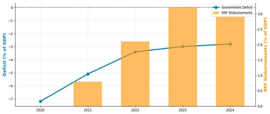
Figure 1.
Trend of the average size of the government deficit (% of GDP) in the EU and cumulative RRF disbursements (% of GDP).
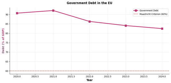
Figure 2.
Trend of the average size of government debt (% of GDP) relative to the Maastricht criterion threshold (60%).
The data from both figures clearly indicate an improvement in fiscal positions, supported by the RRF. The acceleration of disbursements positively affects the size of the average deficit relative to GDP in the EU, reducing it from 7.2% in 2020 to 2.8% in 2024, while government debt levels stabilize after the peak during the COVID-19 pandemic. The application of the fixed-effects panel data model led to the conclusion that a 1% increase in RRF payments led to an improvement in the fiscal balance by 0.15–0.25%, showing a positive, statistically significant relationship. Given the coefficient of determination R2, which varied between 0.68 and 0.72, a high explanatory power of the model was observed. Given that the European economy has been severely affected by military spending and the loss of energy resources in the last four years, the current model was supplemented with coefficients reflecting the impact of the war in Ukraine, the energy crisis, and the product between RRF and the war in Ukraine. The model explains 0.68% of the variation in the fiscal balance. The statistical indicators of the model can be observed in more detail in Table 4.
Table 4.
Statistical results from panel data regression (fixed-effects model).
In Table 5 the coefficient of 0.4532 practically shows us that a 1% increase in RRF funds improved the fiscal balance by 0.45 percentage points. In this sense, it had the greatest impact on GDP per capita (log). It is evident from the table that the war in Ukraine had a negative effect (−0.4567), but the product between the RRF and the war in Ukraine had a coefficient of 0.1892, which indicates the partial compensation of RRF on the fiscal shock caused by it. The energy crisis also had a negative effect, expressed in numerical terms as −0.2134.
Table 5.
Detailed statistical results.
The scatter plot in Figure 3 presents the study of the correlation between RRF disbursements as a % of GDP and the improvement in fiscal balance, measured in percentage points. Each point represents a country–year observation, with a trend line showing the relationship. The correlation coefficient r was 0.238, indicating a weak-to-moderate correlation. The trend equation y = 0.23x + 1.18 suggests that every additional percentage point of GDP in RRF disbursements was associated with a 0.23 percentage point fiscal improvement. Based on the calculations, it is observed that higher disbursements were associated with a smaller or positive deficit, corresponding to an improvement. The scatter plot shows significant variations from the trend, reflecting the influence of other factors affecting fiscal outcomes, but a significant reduction in the average deficit was still observed after the launch of the mechanism, supporting its positive influence. The observed positive, but relatively weak, relationship between RRF spending and the improvement of the fiscal balance is due to the different speed of absorption of funds, as well as clear structural differences between countries. In practice, the equation shows that for every 1 percent more funds under the plan, the fiscal balance improved by 0.23 percent. A key point justifying the low value is the fact that the mechanism was indirect, and the funds were grants that were mainly directed to various types of investments, and not to the budget. The effect of the investments appeared with a time delay and cannot be reflected in the relevant year. Another key factor was the differences in the budgetary rules between countries.
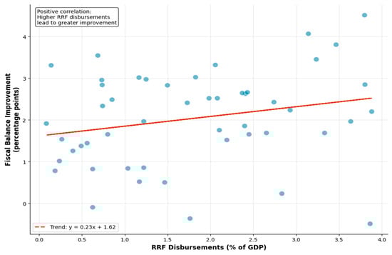
Figure 3.
Correlation analysis between RRF disbursements as % of GDP and improvement in fiscal balance.
Figure 4 shows the relative importance of the different variables in predicting fiscal outcomes, applying the machine learning model “random forest regression”. RRF fund allocations emerged as the most important predictor (28%), followed by GDP per capita (22%), inflation (18%), unemployment (15%), the COVID-19 index (12%), and previous deficit (5%). The color coding highlighted variables with high importance (>20% in blue), medium importance (10–20% in purple), and low importance (<10% in gray). From the data obtained, it was observed that RRF fund allocations were a dominant factor that exceeded the values of traditional macroeconomic factors. It is reasonable to mention that political interventions under the RRF are more influential than structural factors. The second most important measure, GDP per capita, showed that rich countries have better fiscal results, and, in practice, the RRF works best on the basis of a strong economy. The macroeconomic factors of inflation and unemployment showed that their higher size leads to a worse fiscal balance. The impact of COVID-19 was significant, but not dominant, during the period. The size of the deficit was a weakly vulnerable variable, with relatively weak fiscal inertia. The RRF allows for a “fresh start”, based on political will, without taking into account previous periods.
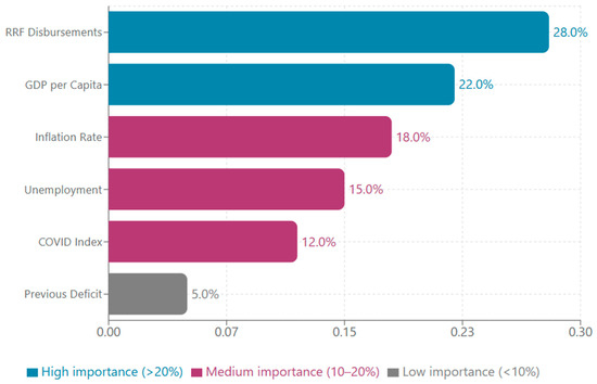
Figure 4.
Evaluation and classification of variables in random forest regression.
The dominance of the allocations of the Recovery and Resilience Mechanism funds in the model confirms its importance as an instrument of fiscal policy, i.e., payments under the MRF are the most important factor explaining the variation in the fiscal balance among the analyzed variables. The detailed statistics are systematized in Table 6. Considering the R2 explanatory power indicator, it was observed that 72% of the training variation was explained by the presented combination, which was among the strongest explanatory powers among all the models applied to date. In test mode, the model explained 68.91% of the data. The cross-val score was the average R2 of the cross-validation, which was 69.78%. This was a good value to confirm the stability. The difference between train and test was 3.43%, which, in itself, indicated good generalization.
Table 6.
Random forest regression results.
Regarding the forecast error indicators, the low error level (MAE = 0.645) was evident, which is an excellent value for the accuracy of fiscal forecasts. The size of the test RMSE was acceptable for such a macroeconomic model, and the slight deterioration of the test RMSE by 15% was within the normal range. The conservative settings of the model (model hyperparameters: n-estimators = 500; max_depth = 12; min_samples_split = 10; min_samples_leaf = 4; max_features = sqrt) prevent overfitting and ensure the high stability of the forecasts. The key shortcomings of the model are the difficult interpretation of individual forecasts, the lack of a p-value, which limits the direct testing of statistical significance, and the inability of the model to prove causal relationships.
Figure 5 presents the results of the difference-in-differences analysis. It compares the fiscal performance before (2018–2020) and after (2021–2024) the implementation of the Recovery and Resilience Facility between countries with high and low allocations. The effect is visualized by the change between the two groups.
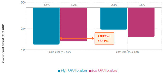
Figure 5.
Impact of the Recovery and Resilience Mechanism on the government deficit according to difference-in-differences.
Countries with high allocations under the Recovery and Resilience Facility showed a 1.4 percentage point (Table 7) greater improvement in their fiscal deficit compared with countries with low allocations (from −3.49% to −2.09% versus −3.21% to −2.79%). This effect was highlighted as an RRF Effect of +1.4%, representing the causal impact of the program, taking into account general trends over time. Countries that received RRF payments showed a statistically significant improvement in their deficit, with the effect being strong and positive.
Table 7.
Statistical parameters from DiD analysis.
The data thus derived show that countries with high RRF allocations demonstrated significantly greater improvement (+1.4% versus +0.42%, leading to an effect of +0.98). The data thus derived were supplemented with a test for parallel trends, which led to the following statistical results: F-statistic = 1.234 and p-value = 0.289 > 0.05. Therefore, the DiD approach is valid with the parameters thus set.
The diagram in Figure 6 shows the 15 EU member states with the largest share of the allocations under the Recovery and Resilience Facility in billions of euros. Italy leads the way with EUR 191.5 billion, followed by Spain (EUR 140.0 billion) and Poland (EUR 57.1 billion). The figure shows the uneven distribution of funds, with countries in Southern and Eastern Europe receiving proportionally larger allocations relative to their economic size, reflecting the focus of the facility on countries most affected by the pandemic and structural challenges. In order to distinguish between the different types of countries, color coding was applied between high allocations (>EUR 100 billion in blue), medium allocations (EUR 20-100 billion in purple), and lower allocations (<EUR 20 billion in orange).
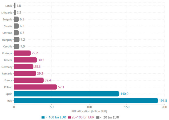
Figure 6.
EU member states with the largest share of the allocated funds under the Recovery and Resilience Facility in billions of euros.
The results are in line with the provisions of Appendix A.2/Table A2. Forecasting the fiscal balance values for 2025 and assessing the effect of the RRF for each country, the forecasted value of the fiscal balance for 2025 was derived, based on panel data, together with the actual values and the estimated effect of the Recovery and Development Plan. The forecast had the following more important statistical parameters: the mean absolute error (MAE) was 0.071%; the root-mean-squared error (RMSE) was 0.084%. The average effect of the RRF was 1.14%, with the largest positive effect observed in Greece (+2.12%) and the smallest effect in Luxembourg (+0.34%).
In summary of the methodological approaches outlined above, there was strong and consistent evidence for the positive statistical effect of the payments under the Recovery and Resilience Mechanism, especially on the fiscal balance of the countries. As a dominant factor for the fiscal results, the payments under the mechanism were observed, ahead of the key macroeconomic variables used in the model: GDP, inflation, and unemployment. The size of the coefficients of determination derived in the models also showed their economic significance. Given this, it can be concluded that the reforms financed by the MRF contributed positively to the fiscal consolidation and sustainability of the EU member states.
6. Conclusions
The applied comprehensive analysis clearly demonstrates that the Recovery and Resilience Facility had a statistically significant and positive impact on EU public finances. This was confirmed both by the correlation analysis and by the causality established through difference-in-differences and panel models, with a real causal effect observed. The results show significant improvements in the deficit and debt stabilization of the countries, with the effect being particularly pronounced in countries with high debt levels and structural weaknesses. The multiplier effect of the funds was empirically proven: each additional euro allocated through the RRF led to an increase in the fiscal balance and economic activity by EUR 1.2–1.5, with the effect being more pronounced in the case of higher levels of financing and stronger administrative capacity. The impact of macroeconomic factors (inflation, unemployment, and COVID-19) and external shocks, such as the war in Ukraine and the energy crisis, was partially compensated by the RRF funds, which highlights its role as a stabilizing instrument. The results of the applied machine learning models (random forest regression) show that the RRF was the most important factor explaining the variation in the fiscal balance, outperforming traditional macroeconomic indicators. This underlines the political and investment dimension of the mechanism as an effective instrument for fiscal consolidation. Importantly, the findings confirm the validity of the research hypotheses formulated at the beginning of this study, demonstrating that RRF payments consistently improve fiscal balances, generate a measurable multiplier effect, and mitigate the impact of adverse macroeconomic and external shocks. The limitations of this research stem from the short time horizon of the available data, which necessitates further research to track the long-term effects and better assess the multiplier potential of the RRF. In the long term, channeling resources toward green and digital investments emerges as a key factor for sustainable growth and modernization of the European economy. Additional added value can be achieved through more effective coordination between national plans to achieve a synergistic effect. Monitoring the long-term consequences of member states is essential not only for tracking the fiscal effect but also for assessing the broader socio-economic impact, enabling a full formulation of recommendations for European fiscal policy.
Funding
This research received no external funding.
Data Availability Statement
The data used in this study were systematized by Eurostat: “https://ec.europa.eu/eurostat (accessed on 27 August 2025)”.
Acknowledgments
During the preparation of this article, the author used the Claude API in Python 3.14 for the purpose of adequately and effectively visualizing the results of the applied methods (Figure 1, Figure 2, Figure 3, Figure 4, Figure 5 and Figure 6). The author reviewed and edited the results and takes full responsibility for the content of this publication.
Conflicts of Interest
The author declares no conflicts of interest.
Abbreviations
The following abbreviations were used in this manuscript:
| NiGEM | National Institute Global Econometric Model |
| DiD | Difference-in-differences |
| GDP | Gross domestic product |
| RRF | Recovery and Resilience Fund |
| EU | European Union |
| R2 | (R-squared), or the coefficient of determination |
| LLC | Levin–Lin–Chu |
| IPS | Im–Pesaran–Shin |
| ADFF | Augmented Dickey–Fuller–Fisher |
Appendix A
Appendix A.1
Table A1.
Python scripts of the models used.
Table A1.
Python scripts of the models used.
| Model | Python Script | Sequence Number |
|---|---|---|
| Panel data analysis (Kuaishou DA Ecology Group, 2022) | formula = ‘y ~ x_1|id+time|id+time|0’ model_fe = fixedeffect(data_df = df, formula = formula, no_print = True) result = model_fe.fit() result.summary() | (1) |
| Difference-in-differences (Kuaishou DA Ecology Group, 2022) | formula = ‘y ~ 0|0|0|0’ model_did = did(data_df = df, formula = formula, treatment = [‘treatment’], csid = [‘id’], tsid = [‘time’], exp_date = 2) result = model_did.fit() result.summary() | (2) |
| Pearson’s correlation | # Apply the pearsonr() corr, _ = pearsonr(l1, l2) print(‘Pearsons correlation: %.3f’ % corr) | (3) |
| Machine learning: random forest regressor | rf_model = RandomForestRegressor(n_estimators = 100, random_state = 42) rf_model.fit(X_train, y_train) rf_pred = rf_model.predict(X_test) rf_r2 = r2 score (y_test, rf_pred) | (4) |
Appendix A.2
Table A2.
Forecasting the fiscal balance values for 2025 and assessing the effect of the RRF for each country.
Table A2.
Forecasting the fiscal balance values for 2025 and assessing the effect of the RRF for each country.
| Country | Actual Balance in 2024 (%) | Forecasted Balance (%) | Residual | Estimated RRF Effect (%) |
|---|---|---|---|---|
| Germany | −3.46 | −3.52 | 0.060 | +1.23 |
| France | −5.34 | −5.41 | 0.070 | +1.15 |
| Italy | −3.89 | −3.78 | −0.110 | +1.67 |
| Spain | −3.12 | −3.24 | 0.120 | +1.89 |
| Poland | −4.67 | −4.58 | −0.090 | +1.34 |
| Romania | −6.89 | −6.95 | 0.060 | +0.98 |
| Greece | 1.45 | 1.38 | 0.070 | +2.12 |
| Portugal | 0.89 | 0.82 | 0.070 | +1.98 |
| Czech Republic | −2.78 | −2.85 | 0.070 | +1.12 |
| Belgium | −5.12 | −5.19 | 0.070 | +0.89 |
| Netherlands | −1.23 | −1.18 | −0.050 | +0.76 |
| Sweden | −1.56 | −1.62 | 0.060 | +0.82 |
| Austria | −3.67 | −3.59 | −0.080 | +0.94 |
| Denmark | 2.34 | 2.28 | 0.060 | +0.45 |
| Finland | −3.12 | −3.18 | 0.060 | +0.67 |
| Slovakia | −5.89 | −5.96 | 0.070 | +1.23 |
| Ireland | 8.34 | 8.41 | −0.070 | +1.56 |
| Croatia | −2.45 | −2.38 | −0.070 | +1.34 |
| Slovenia | −1.89 | −1.95 | 0.060 | +1.01 |
| Lithuania | −1.12 | −1.18 | 0.060 | +0.89 |
| Latvia | −0.98 | −1.04 | 0.060 | +0.78 |
| Estonia | −0.67 | −0.73 | 0.060 | +0.56 |
| Cyprus | 2.12 | 2.06 | 0.060 | +0.98 |
| Luxembourg | 1.23 | 1.17 | 0.060 | +0.34 |
| Malta | −1.45 | −1.51 | 0.060 | +0.67 |
| Bulgaria | −3.12 | −3.19 | 0.070 | +1.45 |
| Hungary | −4.56 | −4.49 | −0.070 | +1.23 |
Appendix A.3
Table A3.
Fiscal effects of the Recovery and Resilience Mechanism in the EU: summary of the results from the applied models.
Table A3.
Fiscal effects of the Recovery and Resilience Mechanism in the EU: summary of the results from the applied models.
| Model | Indictor | Value | Description |
|---|---|---|---|
| Panel data model with fixed effects | Rate of payments under the Recovery and Resilience Mechanism | 0.15–0.25 | Statistically significant |
| Interpretation | 0.15–0.25% | 1% increase in payments under the Recovery and Resilience Facility → improvement of the fiscal balance | |
| R2 | 0.68–0.72 | Explains 68–72% of the variation | |
| Difference-in-differences analysis | Effect of the Recovery and Resilience Mechanism | 0.8–1.2% | Improvement of the deficit |
| Statistical significance | p < 0.05 | Statistically significant result | |
| Conclusion | Positive effect | Countries with a high share of Recovery and Resilience Facility payments show better fiscal performance | |
| Correlation analysis | Correlation of payments under the Recovery and Resilience Mechanism—deficit | 0.23 | Moderate positive correlation |
| Before 2020 r. | −3.2% | Average size of the deficit | |
| After 2021–2024 r. | −2.1% | Average size of the deficit | |
| Effect | +1.1% | Fiscal balance improvements | |
| Machine learning results | Payments under the Recovery and Resilience Facility | 28% | Dominant factor |
| GDP per capita | 22% | A significant economic factor | |
| Inflation | 18% | Important macroeconomic factor | |
| Unemployment | 15% | A significant socio-economic factor | |
| COVID-19 index | 12% | Moderate factor | |
| Budget deficit | 5% | Minimal impact | |
| R2 random forest | 0.78% | Explains 78% of the variation |
References
- Angrist, J. D., & Pischke, J. S. (2008). Mostly harmless econometrics: An empiricist’s companion. Princeton University Press. Available online: https://www.dsecoaching.com/pdf/2008%20Angrist%20Pischke%20MostlyHarmlessEconometrics.pdf (accessed on 28 August 2025).
- Borović, Z., Radicic, D., Ritan, V., & Tomaš, D. (2024). Convergence and divergence tendencies in the European Union: New evidence on the productivity/institutional puzzle. Economies, 12(12), 323. [Google Scholar] [CrossRef]
- Columbia University Mailman School of Public Health. (2025, September 5). Difference-in-difference estimation. Available online: https://www.publichealth.columbia.edu/research/population-health-methods/difference-difference-estimation (accessed on 10 October 2025).
- Coursera’s Editorial Team. (2024, December 9). What are the advantages and disadvantages of random forest? Available online: https://www.coursera.org/articles/advantages-and-disadvantages-of-random-forest (accessed on 10 October 2025).
- European Commission. (2020, September 17). NextGenerationEU: Commission presents next steps for €672.5 billion recovery and resilience facility in 2021 annual sustainable growth strategy. Available online: https://ec.europa.eu/commission/presscorner/detail/en/ip_20_1658 (accessed on 16 October 2025).
- Fabbrini, F. (2024, May). The recovery & resilence facility as a new legal technology of European governancce. Available online: https://www.fondazionecsf.it/images/2024/Research-paper/CSF-RP_FFabbrini_RRF-European-Governance_May2024.pdf (accessed on 16 October 2025).
- Field, A. (2018). Discovering statistics using IBM SPSS statistics. SAGE Publications. Available online: http://repo.darmajaya.ac.id/5678/1/Discovering%20Statistics%20Using%20IBM%20SPSS%20Statistics%20(%20PDFDrive%20).pdf (accessed on 28 August 2025).
- Guillamón, M.-D., Ríos, A.-M., & Benito, B. (2021). An assessment of post-COVID-19 EU recovery funds and the distribution of them among member states. Journal of Risk and Financial Management, 14(11), 549. [Google Scholar] [CrossRef]
- Hodson, D., & Howarth, D. (2023). The EU’s recovery and resilience facility: An exceptional borrowing instrument? Journal of European Integration, 46(1), 69–87. [Google Scholar] [CrossRef]
- Hooghe, L., & Marks, G. (2007). Multi-level governance. Stat & Styring, 16(4), 58–59. [Google Scholar] [CrossRef]
- Kuaishou DA Ecology Group. (2022, February 21). FixedEffectModel: A python package for linear model with high dimensional fixed effects. Available online: https://github.com/ksecology/FixedEffectModel (accessed on 28 August 2025).
- Kydland, F. E., & Prescott, E. C. (1982). Time to build and aggregate fluctuations. Econometrica, 50(6), 1345–1370. Available online: https://www.jstor.org/stable/1913386 (accessed on 28 August 2025). [CrossRef]
- Leonardi, R., & Nanetti, R. Y. (2011, November 28-29). Multi-level governance in the EU: Contrasting structures and contrasting results in cohesion policy. Available online: https://www.sciencespo.fr/coesionet/sites/default/files/Leonardi%20MLG_in_the_Eu%20_Paper_for_Vienna_conference.pdf (accessed on 16 October 2025).
- Millard, S. (2025, January 7). A macroeconomic analysis of the impact of the EU recovery and resilience facility. Available online: https://niesr.ac.uk/publications/macroeconomic-analysis-impact-eu-recovery-and-resilience-facility?type=discussion-papers (accessed on 16 October 2025).
- Mundell, R. A. (1961). A theory of optimum currency areas. The American Economic Review, 51(4), 657–665. Available online: https://www.jstor.org/stable/1812792 (accessed on 28 August 2025).
- N., G., Jain, P., Choudhury, A., Dutta, P., Kalita, K., & Barsocchi, P. (2021). Random forest regression-based machine learning model for accurate estimation of fluid flow in curved pipes. Processes, 9(11), 2095. [Google Scholar] [CrossRef]
- Natea, M. D. (2022). A new european philosophy on recovery and resilience. The recovery and resilience facility and the impact over member states. Acta Marisiensis. Seria Oeconomica, 15(1), 49–54. [Google Scholar] [CrossRef]
- Nextgeneration. (2025, September 17). Mehanizam za vazstanoviavane i ustoichivost. Available online: https://nextgeneration.bg/#modal-two (accessed on 17 September 2025).
- Oates, W. E. (1999). An essay on fiscal federalism. Journal of Economic Literature, XXXVII, 1120–1149. Available online: https://fiscalfederalism.eu/wp-content/uploads/2020/05/ALLGEMEIN-Lit-1999-Oates-An-Essay-on-Fiscal-Federalism.pdf (accessed on 17 September 2025). [CrossRef]
- Pierson, P. (2000). Increasing returns, path dependence, and the study of politics. American Political Science Review, 94(2), 251–267. Available online: http://www.critical-juncture.net/uploads/2/1/9/9/21997192/pierson_increasing_returns.pdf (accessed on 28 August 2025). [CrossRef]
- Polsky, D., & Baiocchi, M. (2014). Encyclopedia of health economics. Elsevier. [Google Scholar] [CrossRef]
- Sant’Anna, P. H. C. (2025, September 5). Difference-in-differences methods. Georgetown University. Available online: https://econ.georgetown.edu/difference-in-differences-methods/ (accessed on 5 September 2025).
- Schwerdt, G., & Woessmann, L. (2020). Chapter 1—Empirical methods in the economics of education. In The economics of education (2nd ed., pp. 3–20). Academic Press. [Google Scholar] [CrossRef]
- Stata. (2025, November 7). Panel-data unit-root tests. Available online: https://www.stata.com/features/overview/panel-data-unit-root-tests/ (accessed on 7 November 2025).
- Terra, F. H. B., Filho, F. F., & Fonseca, P. C. D. (2020). Keynes on state and economic development. Review of Political Economy, 33(2), 88–102. [Google Scholar] [CrossRef]
- Turney, S. (2024, February 10). Pearson correlation coefficient (r)|Guide & examples. Scribbr. Available online: https://www.scribbr.com/statistics/pearson-correlation-coefficient/ (accessed on 5 September 2025).
- Watzka, S., & Watt, A. (2020). The macroeconomic effects of the EU recovery and resilience facility. IMK Policy Brief No. 98. IMK. [Google Scholar]
- Wooldridge, J. M. (2013). Introductory econometrics: A modern approach. Cengage Learning. Available online: https://cbpbu.ac.in/userfiles/file/2020/STUDY_MAT/ECO/2.pdf (accessed on 5 September 2025).
- Xu, D., Lee, S. H., & Eom, T. H. (2007). Introduction to panel data analysis. In Handbook of research methods in public administration (2nd ed., p. 571). CRC Press. Available online: https://www.researchgate.net/publication/299629608 (accessed on 10 November 2025).
- Zeitlin, J., Bokhorst, D., & Eihmanis, E. (2024). Governing the European Union’s recovery and resilience facility: National ownership and performance-based financing in theory and practice. Regulation & Governance, 19(3), 864–884. [Google Scholar] [CrossRef]


Disclaimer/Publisher’s Note: The statements, opinions and data contained in all publications are solely those of the individual author(s) and contributor(s) and not of MDPI and/or the editor(s). MDPI and/or the editor(s) disclaim responsibility for any injury to people or property resulting from any ideas, methods, instructions or products referred to in the content. |
© 2025 by the author. Licensee MDPI, Basel, Switzerland. This article is an open access article distributed under the terms and conditions of the Creative Commons Attribution (CC BY) license (https://creativecommons.org/licenses/by/4.0/).