Abstract
The importance of policy coordination between fiscal and monetary policy authorities has become more apparent, in the face of unexpected economic shocks and persistent macroeconomic challenges. In this paper, we employ the Set-Theoretic Approach (STA) to explicitly measure the presence of coordination between fiscal and monetary policies from 1990 to 2023 in South Africa. In addition, the model measures policy shocks theoretically and structurally using a structural vector autoregressive (SVAR) model. The results indicate a weak level of policy coordination estimated at 24% where shocks are measured theoretically. Where shocks are measured structurally, the results still present weak policy coordination estimated at 33%. These results underscore the need for stronger policy coordination in South Africa, particularly during periods of economic strain such as the Global Financial Crisis and the COVID-19 pandemic, when conflicting fiscal and monetary stances weakened policy effectiveness. In the South African case, limited coordination contributed to procyclical fiscal tightening alongside contractionary monetary policy, which constrained growth and delayed recovery.
1. Introduction
Achieving macroeconomic stability is a central objective for developing countries, underpinning long-term economic growth. It encompasses goals such as full employment, price stability, sustainable debt management, and steady economic expansion (Mankiw, 2021; Dieye, 2020). When effectively managed, stability reduces risks associated with interest rate volatility, fiscal imbalances, and inflation while limiting vulnerability to external shocks (Nasrullah et al., 2023). Yet many developing countries struggle to achieve this objective due to weak institutional frameworks, high debt burdens, persistent price instability, and inequality (Montiel & Servén, 2006). Addressing these challenges requires sound macroeconomic management, structural reforms, improved governance, and greater resilience to external vulnerabilities (World Bank, 2023). At the heart of this effort lie effective fiscal and monetary policies.
Monetary policy (MP), managed by the central bank, influences money supply and interest rates to achieve price stability (Mishkin, 2019). Fiscal policy (FP), directed by the government, focuses on taxation and spending to support growth and social welfare (Martin et al., 2022). Both policies can be used counter-cyclically: expansionary measures during downturns to stimulate growth, and contractionary measures to contain overheating (Blanchard & Johnson, 2022). Their joint ability to influence aggregate demand highlights the importance of coordination.
Policy coordination is the alignment and cooperation between fiscal and monetary authorities, supported by clear frameworks and information sharing (Feng, 2024). While MP and FP have distinct mandates, their complementarity is evident: FP directly shapes demand through spending and taxation, while MP influences investment and consumption via interest rates (Mankiw, 2021). Coordination enables both policies to act accommodatively during recessions without undermining institutional independence (IMF, 2020). Conversely, reliance on either policy in isolation has often proved inadequate in managing volatile and complex economic conditions (Chang, 2024). The importance of coordination became especially apparent during the 2008 Global Financial Crisis (GFC) and the COVID-19 pandemic, when many countries combined fiscal and monetary measures to accelerate recovery (SARB, 2022). However, misaligned objectives can lead to neutralisation or counteractive effects, reducing overall policy effectiveness (Šehović, 2013).
South Africa (SA) illustrates these dynamics clearly. In response to the GFC, fiscal authorities adopted expansionary measures through social and infrastructure spending (Frankel et al., 2008), while the SARB pursued tighter monetary policy to curb capital outflows and maintain price stability (SARB, 2010). This policy divergence slowed recovery and complicated macroeconomic management. By contrast, during the COVID-19 crisis, both authorities pursued accommodative stances: the SARB cut interest rates to support liquidity (SARB, 2020), while the government implemented fiscal packages to mitigate economic damage. Although this coordination aided short-term recovery, it also heightened concerns over inflationary pressures and debt sustainability (Adam et al., 2022).
For developing countries like SA, structural constraints, high inflation, and debt sustainability risks amplify the importance of timely, coordinated policy responses (Davoodi et al., 2021; World Bank, 2022). Comparative experiences reinforce this point. In India, fiscal responsibility legislation has strengthened coordination despite persistent fiscal pressures and inequality (Blagrave & Gonguet, 2020). Brazil, meanwhile, continues to face policy conflicts stemming from high debt and inflation (Sharaf et al., 2024). These examples highlight that for SA, where economic challenges are deep and multifaceted, monetary and fiscal policies cannot be effective if pursued in isolation (Buthelezi, 2023). Against this backdrop, this study’s main objective is explicitly to measure the level of policy coordination in SA.
As its main contribution, this study applies the set-theoretic approach to SA data to measure the degree of policy coordination. Policy shocks are defined structurally and theoretically to enhance the robustness of the findings, allowing for a comparative assessment. The remainder of the study is organised as follows: the next section provides background on the current state of policy coordination in SA. Section 2 reviews the relevant theoretical and empirical literature. Section 3 outlines the data and methodology. Section 4 presents and discusses the empirical results. Finally, Section 5 concludes with key insights and policy recommendations.
Context of SA’s Macroeconomic Policy Coordination
As an emerging market, SA faces persistent structural challenges that constrain economic growth and development (IMF, 2023). High unemployment, driven by skills mismatches and structural rigidities, remains a critical concern. Statistics South Africa (2025) reports youth unemployment at 62.4% and overall unemployment at 32.9% in the first quarter of 2025, exacerbating inequality and poverty. Economic growth and low business confidence, influenced by governance issues and policy uncertainty, further hinder development (National Treasury of South Africa, 2024). Rising public debt and fiscal deficits—debt-to-GDP increasing from 29.6% in 2005 to 76.4% in 2024—limit the government’s capacity to stimulate the economy. As a small open economy, SA is also vulnerable to commodity price swings, interest rate shifts, and geopolitical shocks, highlighting the need for coordinated macroeconomic policies.
Monetary policy (MP) in SA is conducted by the South African Reserve Bank (SARB) through its Monetary Policy Committee (MPC), which meets six times annually to set the repo rate. Operating independently, the SARB’s primary objective is price stability under the inflation-targeting framework adopted in 2000, aiming to maintain inflation within 3–6% while allowing temporary deviations (SARB, 2024). Although MP is independent, it sometimes accommodates fiscal policy (FP) during crises through repo rate adjustments and open market operations, which can facilitate faster recovery but may weaken policy transmission. Figure 1 shows SA’s repo rate from 2000 to 2024, declining from 12% with notable spikes in 2002, and significant cuts during the 2008 GFC and COVID-19 pandemic. SA operates a managed floating exchange rate regime, where market forces largely determine the rand’s value, but the SARB intervenes to mitigate excessive volatility. This regime interacts closely with MP and FP, affecting inflation, trade balances, and capital flows, and underscores the importance of policy coordination in maintaining macroeconomic stability.
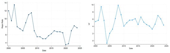
Figure 1.
South Africa’s repo rate and inflation trend. Source: Author’s computation, Data source: SARB.
Fiscal policy (FP) in SA is executed by several key institutions, including the South African Revenue Service (SARS), but the National Treasury holds primary authority over national government finances. The main objectives of FP are to promote long-term economic growth, create employment, reduce income inequality through redistribution, and achieve fiscal consolidation (IMF, 2024). Its principal instruments include taxation, government spending, and public debt management (National Treasury of South Africa, 2021).
Structural and cyclical economic challenges constrain the effectiveness of FP in SA. Low economic growth, high unemployment, persistent poverty, and inequality limit the impact of fiscal interventions. A significant concern has been rising public debt and debt service costs. According to the 2025 Budget Review, debt servicing is projected to reach R1.3 trillion over the next three years, which has necessitated a focus on fiscal consolidation. High debt levels combined with slow growth pose significant risks to macroeconomic stability.
Figure 2 illustrates SA’s debt-to-GDP ratio from 2000 to 2024. Debt levels were low in 2000 due to substantial fiscal consolidation. However, debt and budget deficits rose persistently following the Global Financial Crisis. Slowed growth in the mid-2010s and the economic impact of the COVID-19 pandemic have limited the effectiveness of consolidation efforts, highlighting the ongoing challenge of balancing fiscal sustainability with the need to support economic growth.
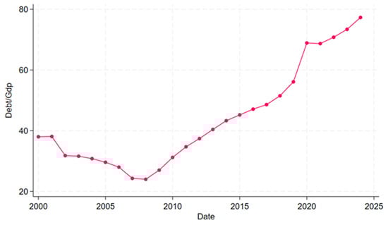
Figure 2.
South Africa’s Debt-to-GDP ratio trend. Source: Author’s computation; Data source: SARB.
The relationship between FP and MP in South Africa is fundamentally interdependent, where the effectiveness of one policy affects the effectiveness of the other policy. Effective MP through stable inflation rates can support FP’s objective of fiscal sustainability by lowering the cost of borrowing, thereby reducing the various ways FP constrains MP (Aron & Muellbauer, 2012).
2. Literature Review
2.1. Theoretical Literature Review
Due to the recent economic crises and structural transformations, the issues of MP and FP coordination have become more pressing, especially for emerging economies (Vitek, 2023). While conventional macroeconomic models have assessed these policies and their effectiveness in bringing about macroeconomic stability independently, recent events have challenged the notion of separation of powers (Englama et al., 2014). Theoretically, the views on policy coordination have evolved over the years, with economists emphasising the need for policy coordination. However, how policy coordination must be conducted has been the primary debate within theoretical and empirical literature. Arby and Hanif (2010) define policy coordination as the process through which monetary and fiscal authorities adjust their policies in a complementary manner to avoid conflicts and improve overall economic outcomes.
Early macroeconomic models strongly favoured the separation of the roles of these policies. The classical dichotomy strongly favours MP as it influences nominal variables, and FP affects real output only in the short run but not in the long run (Mankiw, 2021). Additionally, the Ricardian Equivalence (Barro, 1974) further reduces the effectiveness of FP by suggesting that consumers are forward-looking; therefore, they internalise the government’s budget constraints and adjust their savings accordingly by anticipating future taxes (Isah et al., 2022). Another theory that emphasises the weakness of FP is the rational expectations and time inconsistency models. Kydland and Prescott (1977) and Barro and Gordon (1983) emphasise central bank independence to increase MP credibility and effectiveness. Furthermore, these theories discourage MP and FP coordination, stating that MP can benefit from operational independence by reducing inflationary bias due to FP.
Another line of argument are the researchers who prefer MP dominance. Leeper (1991) defines MP dominance as a theoretical concept where MP is the primary driver of macroeconomic outcomes and FP is constrained to ensure monetary goals are achieved. The New Keynesian, such as the dynamic stochastic general equilibrium model, forms part of the modern macroeconomic models emphasising rule-based policy coordination (Galí, 2015). This model further emphasises that the economy can achieve greater macroeconomic stability by strategically aligning both MP and FP by optimising rule-based policy constraints. Similarly, the Mundell–Fleming model—under floating rates—states that under conditions of unemployment and sticky prices, coordination of MP and FP can stimulate aggregate demand (Siu, 2004). Moreover, under floating exchange rates, MP dominates FP and is more effective at achieving macroeconomic stability. However, these theories do a great job of underscoring the importance and effectiveness of MP. Many criticisms of theories favouring monetary dominance highlight the central bank’s power limitations. Additionally, the assumption is that fiscal authorities will act to support MP goals. Moreover, the developing countries’ economic landscape sometimes makes it difficult for the government to strictly adhere to and operate in a manner that perfectly accommodates MP.
The next approach favours FP and argues that it is the primary driver of macroeconomic outcomes, stating that MP plays a supporting role (Leeper, 1991; Woodford, 1995; Cochrane, 2001; Blanchard, 2021; Cochrane, 2023). The fiscal theory of price level (FTPL) states that the price level is determined by the FP rather than solely by the MP. The price level adjusts to meet the government’s intertemporal budget constraint (Aloui & Guillard, 2019). The Mundell–Fleming model (under fixed exchange rates) and the Modern Monetary Theory (MMT) are other theories supporting the notion that FP determines the price level. The Mundell–Fleming model states that under fixed exchange rates, FP is more effective, and MP should be constrained. Implying that FP should lead in fixed regimes (Karras, 2011). The MMT also emphasises the role of FP in achieving price stability (Liu, 2025). These theories provide greater insight into the importance of FP and its role in achieving macroeconomic stability. The criticism over fiscal dominance has revolved around the concerns that FP may overshadow MP, resulting in uncontrolled inflation and higher debt levels (Jackson, 2024).
The last approach is theories that emphasise the need for strategic coordination by negotiating, cooperating and leadership roles between MP and FP. Strategic coordination theories, particularly the game-theoretic and Stackelberg models, offer great insights into the coordination between MP and FP authorities. The game-theory approach models MP and FP interactions as a cooperative and non-cooperative game that depends highly on the economic context (Zhang, 2024). In regular and recovery periods, MP and FP tend to cooperate, opting for expansionary policy behaviour. During an economic crisis, these policies tend to be in a non-cooperative game, opting for contractionary MP and FP. This coordination of both policies minimises the neutralising effects of a lack of coordination (Saulo et al., 2013).
Theoretical frameworks relevant to the South African context include Leeper (1991), who investigates policy interactions by distinguishing monetary and fiscal dominance. This framework is highly pertinent to SA, where persistent fiscal deficits and increasing government spending limit the SARB’s ability to target inflation (SARB, 2023) independently. According to Leeper, effective coordination requires one authority to act actively while the other remains passive; in SA, fiscal dominance risks constraining monetary policy, highlighting the need for institutional mechanisms to ensure complementarity. Another key perspective is the Mundell–Fleming model, which extends the IS-LM framework to open economies by incorporating the balance of payments curve (Hsing, 2020). This allows for the assessment of policy effectiveness under different exchange rate regimes. For a small open economy like SA with imperfectly flexible prices, monetary policy is more effective under flexible exchange rates. In contrast, fiscal policy is more effective under fixed exchange rates. The model’s emphasis on the sensitivity of money and investment to interest rates is particularly relevant for SA, as high interest rates significantly influence investment decisions and overall economic activity.
2.2. Empirical Literature Review
Earlier studies have often favoured analysing the effectiveness of individual policies in achieving their set objectives. Sargent and Wallace (1981) provide one of the first arguments favouring MP and FP coordination. Though their argument favoured fiscal dominance, stating that high debt levels have significant implications for the MP. This argument sparked further empirical work assessing MP and FP’s interactions and coordination. Given that four different lines of arguments exist concerning policy coordination, the empirical review will be set as such.
Notable studies favouring policy independence include Sargent and Wallace (1981), Debelle and Fischer (1994) and Aron and Muellbauer (2007). These earlier studies provide evidence to support either monetary or fiscal independence, stressing that institutional independence has greater macroeconomic outcomes. A study by Alesina and Summers (1993) employs a cross-country regression analysis on OECD countries, and their key findings show that countries with higher levels of central bank independence experience lower inflation rates. Additionally, a study by Romer and Romer (2004) employs a vector autoregressive (VAR) model to identify the effects of MP shocks on macroeconomic variables. The study’s key findings show that independent monetary actions result in better economic outcomes. Although much recent research has moved more towards policy coordination, schools of thought still favour policy independence and the separation of powers (Bianchi & Melosi, 2017; Bodea & Higashijima, 2017; Debrun & Jonung, 2019).
In the investigation of MP and FP interactions and coordination, there has been evidence that strongly supports active MP frameworks. Much of the existing research favours monetary dominant frameworks for macroeconomic stability, stating that price stability is key to favourable economic outcomes (Gonzalez-Astudillo, 2013). Notably, Chatelain and Ralf (2020) use a theoretical analysis in a Leeper-style model with two equilibrium regimes to compare optimal policy under independent vs. coordinated MP. Their findings suggest better economic outcomes in an economy where MP is active and FP is passive. A recent Cantore and Leonardi (2025) study also employs a New Keynesian DSGE model with liquidity-premium channels. The study further reinforces the need for an MP-driven framework where price stability is the focus, even under fiscal pressure, as a fiscal-driven framework tends to distort the efficiency of MP. Various countries, including India and SA, have adopted approaches prioritising MP frameworks through inflation targeting (Goyal, 2018; SARB, 2020). Moreover, empirical evidence has indicated that unexpected changes in MP have a significant negative economic impact compared to FP changes (Dery & Serletis, 2023).
Many empirical studies aim to determine evidence of the FTPL, which point out the inadequacy of relying on MP-driven frameworks alone to achieve macroeconomic stability (Oboh, 2017). Although evidence points to the effectiveness of MP, most emerging markets are still fiscally dominated. Various empirical studies have found varying results on the impact of FP on the price level. Barrie and Jackson (2022) employ a DSGE model, and their findings indicate that high fiscal deficits are inflationary and result in reduced output and economic growth. This is further reinforced by De Grauwe and Foresti (2023), who have similar findings in their research using a heterogeneous-agent New Keynesian and a standard DSGE model, respectively. While substantial evidence supports that higher fiscal deficits tend to be inflationary, there has been criticism surrounding the FTPL.
Another approach that analyses MP and FP interactions is closely analysing strategic coordination. Game theory is particularly crucial as it provides a framework to model the behaviours of policy coordination (Zhang, 2024). The development of monetary unions, the GFC and the recent COVID-19 pandemic have led to an increase in the interest of MP and FP coordination. Studies by Saulo et al. (2013) and Stawska et al. (2019) use a Nash equilibrium model to analyse the effects of independent policy behaviour in reducing welfare loss. The findings indicate that independent policy behaviour results in sub-optimal outcomes due to a lack of coordination between policy authorities. There is evidence of better macroeconomic outcomes in Brazil when MP leads and FP follows (Saulo et al., 2013). Additionally, a much more recent study by Chibi et al. (2024) employs a dynamic game theory framework to evaluate the interaction between fiscal and monetary policies in Algeria. The findings suggest that the alignment of MP and FP through coordinated and cooperative effort minimises welfare loss and leads to efficient economic shock responses.
The reviewed literature indicates that most existing studies on policy coordination have focused on advanced economies. Most studies within the SA context focus primarily on policy effectiveness (Meyer et al., 2018; Nuru, 2020) instead of policy coordination. Given the macroeconomic outcomes from the GFC and the recent COVID-19 pandemic, it’s crucial to measure policy coordination. It maximises policy effectiveness and assists in identifying institutional weaknesses which hinder the objective of macroeconomic stability (Arby & Hanif, 2010). Moreover, measuring policy coordination can act as a post-crisis evaluation, where evidence has highlighted that countries with higher levels of coordination tend to achieve economic recovery faster (Corsetti et al., 2019). In light of this, the study aims to contribute to existing literature by employing an STA to measure policy coordination levels explicitly across different economic regimes in SA. Furthermore, the scarcity of this analytical framework in the existing literature, combined with the comparative analysis of coordination patterns under alternative shock definitions, enhances the originality and robustness of the findings. The focus on SA is particularly relevant given its inflation-targeting monetary regime, persistent fiscal deficits, rising public debt, and vulnerability to domestic and external shocks, which create a challenging environment for achieving policy alignment.
3. Methodology
The main objective of this study will be to explore the interdependence and to establish the extent of coordination between MP and FP in SA. Policy reaction functions and a set-theoretic approach (STA) will be used to answer this objective. Policy response functions provide various advantages in macroeconomic policymaking, notably MP and FP. A policy reaction function defines how policymakers modify their policy instruments in response to changes in economic conditions (Woodford, 2001). The STA’s benefits lie in its capacity to measure the degree of cooperation between the two policies.
3.1. Institutional Independence—Policy Reaction Functions
Estimating coordination should be valid if there is institutional independence, so it must be established. Policy reaction functions will be estimated to see how FP responds to MP variables and vice versa. Independence is indicated by the FP having a limited response to MP changes, and vice versa. Policy reaction functions describe how policymakers adjust their policy instruments in response to economic shocks or changes in economic conditions. They further capture systematic policy behaviour, showing how key variables are adjusted in reaction to economic shocks (Muscatelli et al., 2004).
Following Afonso et al. (2019), the MP–FP reaction functions are specified. Due to data limitations, however, a modified version of their specification is employed. Unlike Afonso et al. (2019), who use the cyclically adjusted budget balance, our dataset relies on the headline government expenditure, as long as a historical series of cyclically adjusted data and the current account for SA are unavailable. In this framework, the dependent variable represents the primary policy instrument. In contrast, the independent variables include the other authority’s policy instruments and key economic factors—namely the output gap, inflation, the exchange rate, and the long-term interest rate. The MP-FP reaction functions are therefore estimated as follows:
The above Equations (1) and (2) show how the central bank authorities and the government react to economic conditions and how they react to each other. Equation (1) is the MP reaction function, the interest rate is the policy instrument and Equation (2) is the FP reaction function, where the policy instrument is government expenditure.
The Hodrick–Prescott (HP) filter is employed to estimate the output gap. The HP filter uses a statistical tool that decomposes a time series trend, in this case, potential output and a cyclical component, the output gap. The output gap is the deviation of actual output from its potential output level. The equation is specified as follows:
where represents the logarithm of real GDP at time . and denote the potential output and the output gap, respectively. The HP filter estimates the trend component (potential output) by addressing the following optimisation problem:
The first term addresses discrepancies between the actual output and the trend, while the subsequent term mitigates variations in the trend’s growth rate, ensuring smoothness. The smoothing parameter λ governs the trade-off between the fit and the smoothness of the trend. In line with conventional practice for quarterly data, this study sets λ = 1600 (Hodrick & Prescott, 1997).
Table 1 represents the expected signs for the variables included in the policy reaction functions. For the MP reaction function, interest rates and output gap have a positive relationship, where an increase in the output gap will be associated with an increase in the interest rate. Inflation is also expected to positively affect the MP rate, where if there’s an increase in inflation, the central bank’s response would be to increase the interest rate. Additionally, the FP instrument given as government expenditure can have a negative or positive relationship. A negative relationship indicates coordination between MP and FP, and a positive relationship shows independence between the two policies (Afonso et al., 2019).

Table 1.
Policy reaction function and Expected signs.
For the FP reaction function, the MP instrument is given as the interest rate, which, as mentioned for the MP reaction function, can either be positive or negative. A negative sign indicates coordination, and a positive sign indicates independence. A negative relationship is expected between debt and government expenditure. Inflation can be positive or negative, including inflation consistent with the fiscal authority’s need to achieve primary budgetary surpluses. This guarantees that the budget constraint aligns with the price level specified by the monetary authority (Afonso et al., 2019).
3.2. A Set-Theoretic Approach
Several empirical works have favoured using vector autoregressive (VAR) models as an approach to coordination analysis. However, using VAR models with the same variables has proved limiting and often results in conflicting and ambiguous results. A set theoretical approach will be used to achieve this objective. The Set Theoretic Approach (STA) is the work of Arby and Hanif (2010) and Englama et al. (2014), who used the approach. One of the advantages of the STA is its ability to quantify the degree of coordination between the two policies. Arby and Hanif (2010) state that the question of coordination between MP and FP can only arise if operational independence exists between the two institutions. If any decisions or implementations of one of the institutions depend on the actions of the other, then there would be no question of coordination, as it will be ensured. The general perception in the case of the SARB is that it is independent from fiscal authorities.
The STA utilises the set theory to model explicit coordination between the two policies. Two matrices are constructed to model and determine the extent of explicit policy coordination. Once independence has been established, the next step is establishing coordination using the first matrix, which models the macroeconomic environment.
The Macroeconomics Matrix
| TARGETS | Inflation Shocks (Monetary Policy Targets) | ||
| Positive (P) | Negative (N) | ||
| Growth shocks (Fiscal Policy Targets) | Positive (P) | PP | PN |
| Negative (N) | NP | NN | |
As shown in the table above, there are four possible outcomes in the case of monetary and fiscal policy shocks. The first case, represented by “PP”, is an economic condition with only positive shocks to growth and inflation. The second case, represented by “NN”, is a condition whereby growth and inflation are both affected by negative economic shocks. Both these cases are extreme scenarios; however, conflicting scenarios also exist where there might be negative shocks to growth and positive shocks to inflation, vice versa. These are represented by “NP” and “PN” policy environments. Given these shocks, policy behaviour can be indicated by the policy response matrix below.
The Macroeconomic Policy Response Matrix
| POLICY RESPONSE | Monetary Policy Response | ||
| Contraction (C) | Expansion (E) | ||
| Fiscal Policy Response | Contraction (C) | CC | CE |
| Expansion (E) | EC | EE | |
The above table states that if there are positive shocks to both growth and inflation, monetary authorities should adopt a contractionary response to manage inflation and fiscal authorities should follow suit; if not, the policy response should not be expansionary. These are represented by “CC”. When inflation and growth experience negative shocks, monetary and fiscal policy responses should be expansionary, represented by “EE”.
Furthermore, the study employs two methods to measure inflation and growth shocks. The first method will use the sample mean to measure growth shocks and the threshold value to measure inflation shocks. To estimate the inflation threshold value, the study will employ the threshold regression model specified by Hansen (2000). This model allows the effect of inflation on growth to differ depending on whether inflation is above or below an unknown threshold. The model is specified as follows:
where and denotes economic growth and the inflation rate at time t, respectively. is the vector of control variables, where the interest rate is used in this study. and represents the unknown threshold and the error term, respectively. Additionally, and denote the marginal effect of inflation on economic growth below and above the threshold, respectively. is an indicator function equal to 1 if the condition is true and will equal 0 if otherwise.
The second method employs a structural autoregressive (SVAR) model to identify inflation and growth shocks. These structural shocks are incorporated into the interest rate and government expenditure equations within the VAR framework, and their effects are assessed through impulse response functions. Identification is achieved using a Cholesky decomposition of the variance–covariance matrix (Σ) of the reduced-form VAR residuals (). This procedure yields a lower triangular matrix (P), which serves to recover the structural shocks. The Cholesky decomposition of the covariance matrix is specified as follows:
The identified structural shocks are given by
where is a vector of structural shocks, including the inflation shocks and is a vector of structural shocks, including growth shocks.
The stance of MP and FP is interpreted as a change in interest rates and the budget deficit; both variables are adjusted for changes in real GDP and prices. A positive change in the interest rate represents a contractionary MP stance, and a negative change represents an expansionary MP stance. For FP, a positive change in the budget deficit represents an expansionary FP stance, and a negative change represents a contractionary FP stance. Each cell of the macroeconomic environment matrix and policy response matrix reflects a set of those years in which the given combinations of shocks and policy stance have been observed. The extent of coordination is then defined as the following:
where
And refers to the total number of years the study covers. represents the alignment of the 4 quadrants of the macroeconomic matrix and the policy response matrix (e.g., the years in which a positive shock to growth and inflation led to a contractionary response of both MP and FP). can take any value between 0 and 1, where , perfect coordination would occur, and there would be no coordination in the case where . Furthermore, the extent of coordination may or may not emerge due to formal interactions between the monetary and fiscal authorities.
3.3. Data and Variables
For the first method, the data is measured quarterly and ranges from 1990Q4 to 2024Q4. The reason for using quarterly data is that it provides higher frequency observations than annual data. The second method will use annual data ranging from 1990 to 2024. The reason for using annual data is that this approach explicitly measures years of coordination and noncoordination. All data variables are sourced from the SARB.
The variables employed to achieve the study’s objectives include gross domestic product (GDP) growth, government debt and expenditure (both expressed as a percentage of GDP), and the budget deficit (also as a percentage of GDP). The interest rate is measured using the 5-year annual nominal fixed rate on RSA retail savings bonds, reflecting the medium-term monetary policy stance and market expectations beyond short-term fluctuations. The inflation rate captures domestic price pressures, while the real effective exchange rate (REER) reflects external price competitiveness. SA maintains a free-floating exchange rate regime, with the SARB occasionally intervening to smooth excessive volatility rather than target a specific exchange rate level, a practice in place since 2000 (SARB, 2022). Finally, GDP is detrended using the Hodrick–Prescott filter (Hodrick & Prescott, 1997) to compute the output gap.
3.4. Unit Root Test, Lag Selection Tests and Robustness Check
As a preliminary step in working with time series data, the Augmented Dickey–Fuller (ADF) unit root test is conducted to assess the stationarity of the variables. The null hypothesis of the ADF test posits that the series contains a unit root, while the alternative hypothesis indicates that the series is stationary. A variable is considered stationary if the test statistic is more negative than the critical value at conventional significance levels. To identify the structural shocks of inflation and growth, the optimal lag length of the model is determined using the Akaike Information Criterion (AIC) and the Schwarz Criterion (SC). Additionally, to ensure the reliability of the regression results, multicollinearity among the explanatory variables is assessed through pairwise correlations and the Variance Inflation Factor (VIF).
3.5. Limitations
The study faces several limitations. First, although the SARB’s interest rate is often modelled using the inflation target and volatility measures, this study relies on the realised inflation rate in the policy reaction functions to closely follow the approach of Afonso et al. (2019). Second, due to data constraints over the selected period, government expenditure is used as the fiscal variable instead of the cyclically adjusted budget balance. Finally, the treatment of the exchange rate is simplified, and more advanced modelling is recommended for future research.
4. Results and Discussion
To achieve set objectives, this study will use two methods, the first being the establishment of interdependence between the MP and FP variables. The second method will employ the set-theoretic approach specified by Arby and Hanif (2010).
4.1. Interdependence
As standard practice when working with time series data, the establishment of their level of stationarity is essential. This study employs the Augmented Dickey–Fuller to test the stationarity of the data series. Table 2 presents the unit root test results for the variables government debt, budget deficit, government expenditure, and interest rate, showing that the variables are stationary at first difference. The output gap, the real effective exchange rate, and inflation are stationary at I(0).
Table 2.
Unit Root Test Results.
Multicollinearity was assessed using the Variance Inflation Factor (VIF), as VIF provides a precise numerical measure of how much variance in an estimated coefficient is inflated by multicollinearity. Table 3 presents the multicollinearity results, which indicate that all VIF values were comfortably below the threshold of 10, suggesting that multicollinearity is not problematic in the dataset. Overall, multicollinearity does not bias the estimates in a way that would undermine the validity of the findings.
Table 3.
VIF Results.
To establish interdependence, the MP and FP equations are examined to assess how policy decisions affect both MP and FP. The MP and FP reaction functions employed are specified by Equations (2) and (3) (Afonso et al., 2019). An OLS equation model examines the reaction functions. The variables used in the MP reaction function are interest rate, inflation rate, output gap, the real effective exchange rate, and government expenditure, which is the FP variable. Variables included in the FP reaction function are government expenditure, output gap, budget deficit, government debt, and the inflation rate as the MP variable. The output gap is computed using the HP filter and is specified by Equation (1).
Table 4 presents the MP reaction function results; the dependent variable is the interest rate. The results indicate a significant relationship between the past value of the interest rate and its present value, implying that the effects of MP are persistent through the following period. Additionally, the output gap displays a significant positive relationship to the interest rate. This confirms the standard MP rule, which states that a positive output gap increases interest rates to minimise inflation rate hikes (Woodford, 2001). Additionally, this implies that MP reacts to the cyclical conditions of the economy. The inflation rate and the REER negatively affect the interest rate. However, the relationship is significant for the REER and insignificant for the inflation rate. According to Kabundi et al. (2015), to stay consistent with the SARB inflation targeting framework, monetary authorities will increase the interest rate to keep inflation within its 3% to 6% range. To analyse the FP variable, government spending has an insignificant and positive relationship to the interest rate. This positive relationship signifies that MP behaves independently in SA.
Table 4.
Monetary Policy Reaction Function.
Table 5 below presents the FP reaction function results; the dependent variable is government expenditure. The results indicate a statistically insignificant and negative relationship between past government expenditure and its current value. This is in line with the findings by Marire (2022), which suggest that much of the government spending in SA is not on productive investment, resulting in a weak macroeconomic impact. The findings also indicate a statistically significant negative relationship between government spending and the output gap. These results confirm the expected relationship between the two variables, as an increase in government expenditure should significantly decrease the output gap (Auerbach & Gorodnichenko, 2012).
Table 5.
Fiscal Policy Reaction Function.
Furthermore, the inflation rate exhibits a statistically insignificant negative relationship to government expenditure. This could be attributed to the nature of MP in SA, where the SARB maintains a credible inflation-targeting regime (SARB, 2023). Lagged debt exhibits a statistically significant positive relationship to government expenditure, challenging conventional theory. In SA, this relationship reflects the structural persistence of fiscal deficits driven by high recurrent spending and weak economic growth (IMF, 2023). Lastly, the monetary variable analysis shows that FP’s behaviour in SA is coordinated.
The overall results of the MP and FP reaction function point to an independent MP and FP that respond to the conduct of MP in a coordinated manner. MP in SA remains strictly independent through its primary objective of maintaining price stability using the inflation targeting framework. Meanwhile, FP claims to aim for fiscal consolidation to support MP goals.
4.2. The Set Theoretic Approach
The set-theoretic approach uses annual data from 1990 to 2024 to measure the level of coordination in SA explicitly. The data is tested for a unit root as a requirement when using time series data. The ADF is employed to test the stationarity of the data, and the results are presented in Table 6. The interest rate is stationary at the first difference, while the budget deficit, the null hypothesis is rejected at a 10% significance level. This suggests weak evidence of non-stationarity,
Table 6.
Unit Root test results.
The MP and FP variables are the interest rate and the budget deficit as a percentage of GDP, respectively. To establish causality and determine if a long-run relationship exists between the two variables, the Granger Causality and Cointegration tests are conducted. Table 7 presents the results of the Granger causality tests, which show that the interest rate does not Granger-cause the budget deficit, and the budget deficit does not Granger-cause the interest rate. The null hypothesis cannot be rejected at any significance level, implying no causality exists from the interest rate to the budget deficit and vice versa.
Table 7.
Granger Causality tests.
The Phillips–Ouliaris cointegration test is employed to assess the existence of a long-run relationship between the variables. As a residual-based test, it allows for evaluating a stable long-run equilibrium without requiring the estimation a whole vector autoregressive system. The results, reported in Table 8, show no evidence of a long-run relationship between interest rates and budget deficits in SA. A Chow test for structural breaks was conducted to account for potential regime shifts following the GFC. The Chow F-statistic was insignificant at all conventional levels, confirming the stability of the estimated coefficients. Figure 3 illustrates the trends in SA’s interest rates and budget deficits, highlighting periods of co-movement; however, no statistically significant long-run relationship is identified between the two variables.
Table 8.
Cointegration Results. Null hypothesis: No integration between DEFICIT and INT.
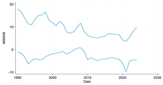
Figure 3.
Interest Rates and Budget Deficit % GDP Trends in South Africa. Source: Author’s computation; Data source: SARB.
Since the interdependence of the MP and FP variables has been established, the next step is to determine the level of coordination between the two policies in SA. The set-theoretic approach presents the degree of coordination using a macroeconomic matrix and a macroeconomic policy response matrix developed by Arby and Hanif (2010). Table 9 reports the values of the growth sample mean, which is given by 6.35% and the inflation threshold, which is 4.10%.
Table 9.
Variable sample mean and threshold results.
Table 10 and Table 11 below display the macroeconomic matrix and the macroeconomic policy responses, respectively. The results of the macroeconomic matrix display the years in which the deviations from the mean and the threshold value were either positive or negative. Specifically, Cell A presents the years in which the deviations from the mean and threshold value were positive. Cell B presents the years in which growth and inflation deviations were positive and negative, respectively. Cell C displays the years when the deviations were negative and positive. Lastly, Cell D displays the years in which growth and inflation deviations were negative. The analysis of the macroeconomics matrix shows that the economy is mainly affected by positive shocks to both inflation and growth for SA. However, a more stable economic condition is characterised by negative shocks to growth and positive shocks to inflation. Empirical research suggests the characterisation of the South African economy as experiencing negative growth shocks alongside positive inflation shocks, often resulting in a stagflation-like economic condition (Sangweni & Ngalawa, 2023). Buthelezi (2023) states that negative growth shocks stem from supply-side challenges and structural inefficiencies, while positive inflation shocks stem from demand-side pressures and commodity price volatility.
Table 10.
The macroeconomic matrix.
Table 11.
The macroeconomic Policy Response matrix.
Table 11 displays the macroeconomic policy response matrix. This matrix shows MP and FP responses to growth and inflation shocks presented in Table 10. Cell A presents the years when a positive macroeconomic shock decreased interest rates and fiscal deficits, implying a contractionary response from both MP and FP. Cell B presents the years in which interest rates increased, and the budget deficit decreased. Cell C presents the years in which interest rates decreased, and the budget deficit increased in response to economic shocks. Lastly, Cell D presents the years in which negative shocks increased the interest rate and the budget deficits. The results suggest that the South African economy is characterised by an expansionary and a contractionary FP. Additionally, when negative growth and positive inflation shocks exist, the economy has leaned towards expansionary FP and contractionary MP over the years.
Table 12 displays the years of coordination and noncoordination; the degree of coordination is computed as specified by Equation (9). According to the results, the extent of coordination between MP and FP in SA for this study period is 24%. This points to a weak level of coordination in SA for this study period. This aligns with the findings by Aron and Muellbauer (2007), who investigate the policy effectiveness in SA; their findings indicate a weak level of coordination and emphasise the counterproductive effects of poor coordination, especially during economic shocks.
Table 12.
Coordination Results.
To further the analysis, this approach defines and analyses structural shocks to inflation and growth as specified by Equation (5). This assists in looking at the response of inflation to structural shocks rather than a deviation from a threshold value. Additionally, growth responds to structural shocks rather than the simple mean. In measuring structural shocks, the AIC/SC lag selection results are presented in Table 13 below.
Table 13.
Lag Selection Results.
Table 14 presents the macroeconomic matrix and its results. The response of inflation to structural shocks was positive from 1990 to 1994, and subsequently, it has been negative in the remaining years. Its response to structural shocks has only been positive for growth for this study period. Additionally, in the analysis Table 15 presents the macroeconomic policy response, the findings are the same as the macroeconomic policy response matrix given in Table 9 above. The findings allude to an expansionary MP in response to positive growth shocks and negative inflation shocks.
Table 14.
The macroeconomic matrix.
Table 15.
The macroeconomic policy response matrix.
In comparison, FP is mainly expansionary in the presence of negative growth and positive inflation shocks. Table 16 presents the years of coordination and noncoordination for this study period. With Equation (5), the extent of coordination when using structural shocks for inflation and growth is calculated to be 33%. This is slightly higher than the other method, which measures inflation shocks as deviations from the threshold value and growth shocks as deviations from the sample mean. However, the values still indicate a weak level of coordination for SA, with the difference between the two approaches being 9%.
Table 16.
Coordination Results.
5. Conclusions
The study starts by establishing interdependence between MP and FP in SA. This is done by employing the MP rule and FP rule equations. The results indicate that the fiscal variable proxied as government spending has an insignificant and positive relationship to the interest rate for the MP equation. This supports empirical evidence that the transmission mechanism between FP and MP may be weak due to economic rigidities (Kabundi & Mbelu, 2018). On the other hand, for the FP equation, the monetary variable proxied as the inflation rate exhibits a statistically insignificant negative relationship to government expenditure. This is expected, as SA has adopted an inflation-targeting framework which aims to stabilise the price level in the economy. Subsequently, a cointegration test must determine a long-term relationship between the MP (interest rate) and the FP (deficit) variables. The results indicate no evidence of a long-run relationship between interest rates and budget deficits in the case of SA. This is consistent with the evidence by Jooste et al. (2013), which suggests that no consistent causality long-run relationship exists between contractionary MP and deficits in SA. The first approach of the STA, which uses theoretical shocks, shows weak policy coordination in SA, which is estimated at 24% for the period. The second approach still shows the presence of weak policy coordination in SA, which is estimated to be slightly higher at 33% when shocks are measured structurally. This could be attributed to the ability of the SVAR to provide more robust results, as it can differentiate between temporary and persistent shocks to inflation and growth.
In SA, crisis responses over the past two decades were often fragmented, illustrating the importance of coordinated policy. During 2007–2009, monetary easing coincided with a cautious fiscal stance; in 2020–2021, the SARB introduced unconventional measures while fiscal relief was implemented without coordinated timing or a credible financing plan, leading to offsetting exchange-rate and interest-rate effects; and in 2022–2023, high debt constrained fiscal support while monetary tightening curtailed growth (SARB, 2023). Weak coordination can be attributed to SARB’s inflation-targeting independence, high and rising public debt, and the absence of institutional mechanisms for joint decision-making (Sangweni & Ngalawa, 2023). An optimal crisis strategy would combine targeted, temporary fiscal expansion with accommodative monetary policy, followed by gradual tightening. Broader SARB actions, including liquidity provision and bond purchases, further shape macroeconomic outcomes. Without formal alignment, the stabilising impact of both policies remains limited, underscoring the need for credible sequencing and coordination to maximise stimulus effectiveness and maintain macroeconomic stability.
Author Contributions
Conceptualization A.M., M.C.N. and S.M.; methodology, A.M., M.C.N. and S.M.; validation, A.M.; formal analysis A.M., M.C.N. and S.M.; investigation, A.M., M.C.N. and S.M.; resources, A.M., M.C.N. and S.M.; data curation, A.M., M.C.N. and S.M.; writing—original draft preparation, A.M., M.C.N. and S.M.; writing—review, A.M., M.C.N. and S.M.; visualization, A.M. supervision, M.C.N. and S.M. All authors have read and agreed to the published version of the manuscript.
Funding
This research received no external funding.
Data Availability Statement
The data used in the study is publicly available on the South African Reserve Bank repository.
Acknowledgments
I wish to thank the UKZN Masters and PhD cohort for their academic support and my loved ones for their personal encouragement throughout this journey.
Conflicts of Interest
The authors declare no conflict of interest.
Correction Statement
This article has been republished with a minor correction to the Data Availability Statement. This change does not affect the scientific content of the article.
References
- Adam, C., Alberola-Ila, E., & Tejada, A. P. (2022). COVID-19 and the monetary-fiscal policy nexus in Africa. In BIS papers. Bank for International Settlements. [Google Scholar]
- Afonso, A., Alves, J., & Balhote, R. (2019). Interactions between monetary and fiscal policies. Journal of Applied Economics, 22(1), 132–151. [Google Scholar] [CrossRef]
- Alesina, A., & Summers, L. H. (1993). Central bank independence and macroeconomic performance: Some Comparative evidence. Journal of Money, Credit and Banking, 25(2), 151–162. [Google Scholar] [CrossRef]
- Aloui, R., & Guillard, M. (2019). Interaction between monetary and fiscal policies in the presence of sovereign risk. Economic Modelling, 80, 494–508. [Google Scholar]
- Arby, M. F., & Hanif, M. N. (2010). Monetary and fiscal policies coordination—Pakistan’s experience. SBP Research Bulletin, State Bank of Pakistan, 6(1), 3–13. [Google Scholar]
- Aron, J., & Muellbauer, J. (2007). Review of monetary policy in South Africa Since 1994. Journal of African Economies, 16(5), 705–744. [Google Scholar] [CrossRef]
- Aron, J., & Muellbauer, J. (2012). Monetary policy and inflation modelling in a more open economy in South Africa. Economic Modelling, 29(3), 938–956. [Google Scholar]
- Auerbach, A. J., & Gorodnichenko, Y. (2012). Measuring the Output Responses to Fiscal Policy. American Economic Journal: Economic Policy, 4(2), 1–27. [Google Scholar]
- Barrie, M. S., & Jackson, E. A. (2022). The impact of fiscal dominance on macroeconomic performance in Sierra Leone: A DSGE simulation approach. West African Journal of Monetary and Economic Integration, 22(1), 1–33. [Google Scholar]
- Barro, R. J. (1974). Are government bonds net wealth? Journal of Political Economy, 82(6), 1095–1117. [Google Scholar] [CrossRef]
- Barro, R. J., & Gordon, D. B. (1983). Rules, discretion and reputation in a model of monetary policy. Journal of Monetary Economics, 12(1), 101–121. [Google Scholar] [CrossRef]
- Bianchi, F., & Melosi, L. (2017). Escaping the great recession. American Economic Review, 107(4), 1030–1058. [Google Scholar] [CrossRef]
- Blagrave, P., & Gonguet, F. (2020). Enhancing fiscal transparency and Reporting in India.
- Blanchard, O. (2021). Public debt and low interest rates. American Economic Review, 111(1), 1–26. [Google Scholar]
- Blanchard, O., & Johnson, D. R. (2022). Macroeconomics (8th ed.). Pearson. [Google Scholar]
- Bodea, C., & Higashijima, M. (2017). Central bank independence and fiscal policy: Can the central bank restrain deficit spending? British Journal of Political Science, 47(1), 47–70. [Google Scholar] [CrossRef]
- Buthelezi, E. M. (2023). Impact of government expenditure on economic growth in different states in South Africa. Cogent Economics & Finance, 11(1), 2209959. [Google Scholar] [CrossRef]
- Cantore, C., & Leonardi, E. (2025). Monetary–fiscal interaction and the liquidity of government debt. European Economic Review, 173, 104979. [Google Scholar] [CrossRef]
- Chang, Z. (2024). How to coordinate the roles of fiscal policy and monetary policy. GBP Proceedings Series, 1. Available online: https://www.gbspress.com/index.php/GBPPS (accessed on 16 June 2025). [CrossRef]
- Chatelain, J. B., & Ralf, K. (2020). Ramsey optimal policy versus multiple equilibria with Fiscal and Monetary interactions. arXiv, arXiv:2002.04508. [Google Scholar] [CrossRef]
- Chibi, A., Zahaf, Y., & Chekouri, S. M. (2024). Strategic interaction between monetary and fiscal policy in Algeria: A game theory approach. International Journal of Business and Economic Studies, 6(4), 262–280. [Google Scholar] [CrossRef]
- Cochrane, J. H. (2001). Long-term debt and optimal policy in the fiscal theory of the price level. Econometrica, 69(1), 69–116. [Google Scholar] [CrossRef]
- Cochrane, J. H. (2023). The fiscal theory of the price level. Princeton University Press. [Google Scholar]
- Corsetti, G., Dedola, L., Jarociński, M., Maćkowiak, B., & Schmidt, S. (2019). Macroeconomic stabilization, monetary-fiscal interactions, and Europe’s monetary union. European Journal of Political Economy, 57, 22–33. [Google Scholar] [CrossRef]
- Davoodi, H. R., Montiel, P. J., & Ter-Martirosyan, A. (2021). Macroeconomic stability and inclusive growth. IMF Working Paper. International Monetary Fund. [Google Scholar]
- Debelle, G., & Fischer, S. (1994). How independent should a central bank be? In J. C. Fuhrer (Ed.), Goals, guidelines, and constraints facing monetary policymakers (pp. 195–221). Federal Reserve Bank of Boston. [Google Scholar]
- Debrun, X., & Jonung, L. (2019). Under threat: Rules-based fiscal policy and how to preserve it. European Journal of Political Economy, 57, 142–157. [Google Scholar] [CrossRef]
- De Grauwe, P., & Foresti, P. (2023). Interactions of fiscal and monetary policies under waves of optimism and pessimism. Journal of Economic Behavior & Organization, 212, 466–481. [Google Scholar] [CrossRef]
- Dery, C., & Serletis, A. (2023). Macroeconomic fluctuations in the United States: The role of monetary and fiscal policy shocks. Open Economics Review. online ahead of print. [Google Scholar] [CrossRef]
- Dieye, A. (2020). Overview of current macroeconomic policy issues and challenges in mainstream economics. In An Islamic model for stabilization and growth (pp. 11–47). Palgrave Macmillan. [Google Scholar] [CrossRef]
- Englama, A., Tarawalie, A. B., & Ahortor, C. R. (2014). Fiscal and monetary policy coordination in the WAMZ: Implications for member states’ performance on the convergence criteria. In Private sector development in West Africa (pp. 61–94). Springer International Publishing. [Google Scholar]
- Feng, Z. (2024). Research on the coordination mechanism of fiscal and monetary regulation. International Journal of Global Economics and Management, 4(2), 16–22. [Google Scholar] [CrossRef]
- Frankel, J., Smit, B., & Sturzenegger, F. (2008). South Africa: Macroeconomic challenges after a decade of success. Economics of Transition, 16(4), 639–677. [Google Scholar] [CrossRef][Green Version]
- Galí, J. (2015). Monetary policy, inflation, and the business cycle: An introduction to the new Keynesian framework and its applications (2nd ed.). Princeton University Press. [Google Scholar]
- Gonzalez-Astudillo, M. (2013). Monetary-fiscal policy interactions: Interdependent policy rule coefficients.
- Goyal, A. (2018). The Indian fiscal-monetary framework: Dominance or coordination? International Journal of Development and Conflict, 8(1), 1–13. [Google Scholar]
- Hansen, B. E. (2000). Sample splitting and threshold estimation. Econometrica, 68(3), 575–603. [Google Scholar] [CrossRef]
- Hodrick, R. J., & Prescott, E. C. (1997). Postwar U.S. business cycles: An empirical investigation. Journal of Money, Credit and Banking, 29(1), 1–16. [Google Scholar] [CrossRef]
- Hsing, Y. (2020). Does the Mundell-Fleming model apply to South Africa? Journal of Management and Business, 6(2), 89–98. [Google Scholar]
- International Monetary Fund (IMF). (2020). Fiscal monitor: Policies for the recovery. IMF. [Google Scholar]
- International Monetary Fund (IMF). (2023). Fiscal monitor: On the path to policy normalization. IMF. [Google Scholar]
- International Monetary Fund (IMF). (2024). South Africa: Staff concluding statement of the 2024 Article IV mission. International Monetary Fund. Available online: https://www.imf.org/en/News/Articles/2024/11/26/mcs-south-africa-staff-concluding-statement-of-the-2024-article-iv-mission (accessed on 13 August 2025).
- Isah, A., Joseph, T., & Dairo, R. (2022). Review of Ricardian equivalence in theory and practice: Empirical data from Nigeria. Applied Journal of Economics, Management and Social Sciences, 3(1). [Google Scholar] [CrossRef]
- Jackson, E. A. (2024). Economics of fiscal dominance and ramifications for the discharge of effective monetary policy transmission. SSRN Electronic Journal. Preprint. [Google Scholar] [CrossRef]
- Jooste, C., Liu, G. D., & Naraidoo, R. (2013). Analysing the effects of fiscal policy shocks in the South African economy. Economic Modelling, 32, 215–224. [Google Scholar] [CrossRef]
- Kabundi, A., & Mbelu, A. (2018). Has the exchange rate pass-through changed in South Africa? South African Journal of Economics, 86(3), 339–360. [Google Scholar] [CrossRef]
- Kabundi, A., Schaling, E., & Some, M. (2015). Monetary policy and heterogeneous inflation expectations in South Africa. Economic Modelling, 45, 109–117. [Google Scholar] [CrossRef]
- Karras, G. (2011). Exchange-rate regimes and the effectiveness of fiscal policy. Journal of Economic Integration, 26(1), 29–44. [Google Scholar] [CrossRef]
- Kydland, F. E., & Prescott, E. C. (1977). Rules rather than discretion: The inconsistency of optimal plans. Journal of Political Economy, 85(3), 473–491. [Google Scholar] [CrossRef]
- Leeper, E. M. (1991). Equilibria under ‘active’ and ‘passive’ monetary and fiscal policies. Journal of Monetary Economics, 27(1), 129–147. [Google Scholar] [CrossRef]
- Liu, Y. (2025). Can Modern Monetary Theory fit the post-Crisis US facts? Evidence from a full DSGE model. International Journal of Finance & Economics, 30(1), 983–1006. [Google Scholar]
- Mankiw, N. G. (2021). Principles of economics (9th ed.). Cengage Learning. [Google Scholar]
- Marire, J. (2022). Relationship between fiscal deficits and unemployment in South Africa. Journal of Economic and Financial Sciences, 15(1), 693. [Google Scholar] [CrossRef]
- Martin, T., Ondra, V., & Dominik, K. (2022). The role of fiscal vs. monetary policy in modern economics. Fusion of Multidisciplinary Research, An International Journal, 3(2), 2022. Available online: https://fusionproceedings.com/fmr/1/article/view/40 (accessed on 28 February 2025). [CrossRef]
- Meyer, D. F., De Jongh, J., & Van Wyngaard, D. (2018). An assessment of the effectiveness of monetary policy in South Africa. Acta Universitatis Danubius. Œconomica, 14(6). [Google Scholar]
- Mishkin, F. S. (2019). The economics of money, banking, and financial markets (12th ed.). Pearson. [Google Scholar]
- Montiel, P., & Servén, L. (2006). Macroeconomic stability in developing countries: How much is enough? The World Bank Research Observer, 21(2), 151–178. [Google Scholar] [CrossRef]
- Muscatelli, V. A., Tirelli, P., & Trecroci, C. (2004). Fiscal and monetary policy interactions: Empirical evidence and optimal policy using a structural New-Keynesian model. Journal of Macroeconomics, 26(2), 257–280. [Google Scholar] [CrossRef]
- Nasrullah, M. J., Saghir, G., shahid Iqbal, M., & Hussain, P. (2023). Macroeconomic Stability and Optimal Policy Mix. iRASD Journal of Economics, 5(3), 725–745. [Google Scholar] [CrossRef]
- National Treasury of South Africa. (2021). Medium term budget policy statement 2021. National Treasury. [Google Scholar]
- National Treasury of South Africa. (2024). Budget review 2024. National Treasury. [Google Scholar]
- Nuru, N. Y. (2020). Monetary and fiscal policy effects in South African economy. African Journal of Economic and Management Studies, 11(4), 625–638. [Google Scholar] [CrossRef]
- Oboh, V. U. (2017). Monetary and fiscal policy coordination in Nigeria: A dynamic approach. Central Bank of Nigeria Journal of Applied Statistics, 8(1), 1–16. [Google Scholar]
- Romer, C. D., & Romer, D. H. (2004). A new measure of monetary shocks: Derivation and implications. American Economic Review, 94(4), 1055–1084. [Google Scholar] [CrossRef]
- Sangweni, S. D., & Ngalawa, H. (2023). Inflation dynamics in South Africa: The role of public debt. Journal of Economic and Financial Sciences, 16(1), 750. [Google Scholar] [CrossRef]
- Sargent, T. J., & Wallace, N. (1981). Some unpleasant monetarist arithmetic. Federal Reserve Bank of Minneapolis Quarterly Review, 5(3), 1–17. [Google Scholar] [CrossRef]
- Saulo, H., Rêgo, L. C., & Divino, J. A. (2013). Fiscal and monetary policy interactions: A game theory approach. Annals of Operations Research, 206(1), 341–366. [Google Scholar] [CrossRef]
- Šehović, D. (2013). General aspects of monetary and fiscal policy coordination. Journal of Central Banking Theory and Practice, 2(3), 5–27. [Google Scholar]
- Sharaf, M. F., Shahen, A. M., & Binzaid, B. A. (2024). Asymmetric and nonlinear foreign debt–inflation nexus in Brazil: Evidence from NARDL and Markov regime switching approaches. Economies, 12(1), 18. [Google Scholar] [CrossRef]
- Siu, H. E. (2004). Optimal fiscal and monetary policy with sticky prices. Journal of Monetary Economics, 51(3), 575–607. [Google Scholar] [CrossRef]
- South African Reserve Bank (SARB). (2010). Annual report 2009/10. South African Reserve Bank. [Google Scholar]
- South African Reserve Bank (SARB). (2020). Our response to COVID-19. South African Reserve Bank. Available online: https://www.resbank.co.za/en/home/publications/publication-detail-pages/media-releases/Our-response-to-COVID-19 (accessed on 10 August 2025).
- South African Reserve Bank (SARB). (2022). Monetary and fiscal policy interactions in the wake of the COVID-19 pandemic. [online]. South African Reserve Bank. Available online: https://www.resbank.co.za (accessed on 12 June 2025).
- South African Reserve Bank (SARB). (2023). Is South Africa falling into a fiscal dominant regime? Working Paper WP/23/02. South African Reserve Bank. [Google Scholar]
- South African Reserve Bank (SARB). (2024). Inflation targeting framework. [online]. Available online: https://www.resbank.co.za/en/home/what-we-do/monetary-policy/inflation-targeting-framework (accessed on 10 June 2025).
- Statistics South Africa. (2025). Quarterly Labour Force Survey (QLFS)—Q1: 2025 [Media release]. Pretoria. Statistics South Africa. Published 13 May 2025. [Google Scholar]
- Stawska, J., Malaczewski, M., & Szymańska, A. (2019). Combined monetary and fiscal policy: The Nash Equilibrium for the case of non-cooperative game. Economic research-Ekonomska istraživanja, 32(1), 3554–3569. [Google Scholar] [CrossRef]
- Vitek, M. F. (2023). Measuring the stances of monetary and fiscal policy. International Monetary Fund. [Google Scholar]
- Woodford, M. (1995). Price level determinacy without control of a monetary aggregate. Carnegie-Rochester Conference Series on Public Policy, 43, 1–46. [Google Scholar] [CrossRef]
- Woodford, M. (2001). Fiscal requirements for price stability. Journal of Money, Credit and Banking, 33(3), 669–728. [Google Scholar] [CrossRef]
- World Bank. (2022). Global economic prospects, June 2022. World Bank. [Google Scholar]
- World Bank. (2023). Global economic prospects, January 2023: A fragile recovery. World Bank. [Google Scholar]
- Zhang, E. (2024). Coordination of monetary and fiscal policies from a game theoretic perspective. Advances in Economics, Management and Political Sciences, 107(1), 10–14. [Google Scholar] [CrossRef]


Disclaimer/Publisher’s Note: The statements, opinions and data contained in all publications are solely those of the individual author(s) and contributor(s) and not of MDPI and/or the editor(s). MDPI and/or the editor(s) disclaim responsibility for any injury to people or property resulting from any ideas, methods, instructions or products referred to in the content. |
© 2025 by the authors. Licensee MDPI, Basel, Switzerland. This article is an open access article distributed under the terms and conditions of the Creative Commons Attribution (CC BY) license (https://creativecommons.org/licenses/by/4.0/).