The Asymmetric Effects of Unemployment and Output on Inflation in Greece: A Nonlinear ARDL Approach

Abstract

This study examines the asymmetrical effects of unemployment and output on inflation in Greece. It applies a nonlinear autoregressive distributed lag model to focus on how positive and negative economic indicator fluctuations impact inflation. The empirical findings indicate an asymmetric and inverse relationship between inflation and unemployment. In the long run, positive shocks to unemployment affect inflation with greater intensity than negative shocks. The short-run trade-off between unemployment and inflation demonstrates linearity, with inflation showing greater sensitivity and a tendency to increase more during periods of economic expansion. Additionally, we find a nonlinear and positive relationship between inflation and output in both the long and short run. In the long run, negative output shocks have a more significant impact on inflation than positive shocks, while in the short run the results are reversed. These findings suggest that policymakers should carefully consider the nonlinearities of the Phillips curve to avoid policy errors in macroeconomic models.

1. Introduction

The link between real economic activity and inflation has been one of macroeconomics’ most controversial theoretical and empirical issues. Phillips (1958) examined the trade-off between inflation and slack in the economy and found a negative relationship between inflation and unemployment, known as the Phillips curve. Subsequent research has been critical and refined this concept, with studies by Samuelson and Solow (1960), Phelps (1967), Friedman (1968), Lucas (1973), Dixon (1988), Caballero and Hammour (1994), and Pissarides (2000, 2013), among others, building upon and modifying the original findings to create a more nuanced understanding of this crucial relationship.

Many economists have long argued that the Phillips curve has evolved considerably in recent years. Numerous studies since the 1980s have suggested that the curve is nonlinear and convex, indicating that inflation may react differently to changes in unemployment depending on whether it is above or below the natural unemployment rate. Research indicates that the slope of the Phillips curve has become flatter over time (Ball and Mazumder 2011; International Monetary Fund 2013; Blanchard et al. 2015; Coibion and Gorodnichenko 2015; Del Negro et al. 2020; Harding et al. 2023). One possible reason for these nonlinearities is the impact of anchored inflation expectations (Orphanides and Williams 2005; McLeay and Tenreyro 2020; Ascari and Fosso 2021; Jorgensen and Lansing 2024). This perspective suggests that inflation has become lower and more persistent, with recessions potentially creating stronger disinflationary pressures that are harder for central banks to manage. Evidence indicates that inflation expectations have become less volatile since the 1990s. Additionally, factors such as shifts in labor market conditions, technological progress, and globalization may also account for the nonlinearities observed in the Phillips curve (Ciccarelli and Mojon 2010; Gürkaynak et al. 2010; Jašová et al. 2018; Del Negro et al. 2020; Ratner and Sim 2022; Ahn and Lee 2023). A notable change in the labor market, contributing to the flattening of the curve, is the decrease in workers’ bargaining power since the 1980s. Globalization and technological progress have influenced domestic inflation by providing cheaper imports, increasing competition, and enhancing efficiency, resulting in more stable prices despite variations in unemployment and labor market conditions. Previous studies have indicated that a convex Phillips curve necessitates a much tighter monetary policy than a linear one (Kumar and Orrenius 2016). While a linear Phillips curve suggests a balanced monetary policy response to periods of excess demand or supply, a nonlinear curve may require preemptive actions to combat inflation, particularly when unemployment falls below the natural rate (Macklem 1997; Laxton et al. 1999; Boehm and Pandalai-Nayar 2022). In an overheated economy, a convex Phillips curve means that larger declines in output are necessary to control inflation. This highlights the advantages of adopting proactive monetary policy measures before the economy overheats, as delaying action can be costly. Economies with a flatter (steeper) Phillips curve tend to have relatively rigid (flexible) wages, resulting in greater (lesser) impacts from contractionary monetary policy. Similarly, during periods of high unemployment, expansionary policies are likely to be less inflationary than anticipated (Gross and Semmler 2019).

In recent years, the world economy has faced several crises, such as the global economic crisis, the COVID-19 pandemic, and most recently, the energy crisis, creating uncertainty among economic agents and affecting macroeconomic indicators (Al-Nassar and Albahouth 2023). The economic recession that began towards the end of 2007, commonly known as the “Great Recession”, was characterized by a significant fall in economic activity and a swift rise in unemployment rates. However, from 2008 to 2010, the significant decrease in output and increase in unemployment were not accompanied by a substantial drop in inflation. The economic recovery period and unemployment decline were interrupted by the unexpected shock of the COVID-19 pandemic in 2020. Nevertheless, as for 2008–2010, the traditional Phillips curve was not fully observed during the pandemic. While unemployment reached an all-time high during the early months of the pandemic, inflation did not fall as much as expected (Haschka 2024). Following the lifting of lockdown measures, the substantial increase in consumption, heightened energy demands, and problems in the global supply chain created further inflationary pressures in the economy. The aftermath of the pandemic shock led to a significant and sustained increase in inflation during 2021–2022, exacerbated by the energy crisis and the war in Ukraine. This unusually high inflation rate caused great uncertainty among economists about future developments. All these fluctuations in inflation during the last decades can be attributed to nonlinearities in the Phillips curve within business cycles, indicating the asymmetrical responses of inflation to economic activity (Passamani et al. 2022). It is crucial to investigate how an economy reacts to both positive and negative shocks at different stages of the business cycle, especially for policymakers, who need to identify the causes of inflationary pressures and develop effective strategies to maintain price stability (Forbes et al. 2021; Ball et al. 2021). Adopting a linear Phillips curve in macroeconomic models may indicate substantial weaknesses that could result in the implementation of ineffective policies (Gagnon and Sarsenbayev 2022; Benigno and Eggertsson 2023).

In this context, this paper focuses on the case of Greece for several reasons. The adoption of the euro initially reduced uncertainty in Eurozone countries, but over time, disparities between member states appeared in various macroeconomic indicators, specifically at the beginning of the global economic crisis. From 1998 to 2007, the Greek economy faced extremely favorable conditions, such as high GDP growth, low interest rates, primary surpluses until 2003, privatization revenues, and low unemployment. However, after 2007, the GDP experienced a significant decline. The economic crisis caused the public debt to soar and exacerbated existing macroeconomic imbalances in the Greek economy, including low international competitiveness and high labor costs due to low productivity. Greece implemented strict fiscal policies and structural reforms after joining the support mechanism (European Commission, European Central Bank, International Monetary Fund) in 2010. Compared to other European Union (EU) countries, Greece experienced a deeper recession and higher unemployment rates. Greece had the highest unemployment rate and the biggest GDP decline among the EU countries for many years after the start of the global economic crisis. The focus on reducing the country’s high debt combined with commitments to achieve high primary surpluses constrained the country’s ability to implement expansionary and growth-oriented economic strategies that could have alleviated the high levels of unemployment. In the context of these challenges, addressing the high unemployment rates in Greece necessitated structural reforms on the supply side, particularly focusing on the labor market structure. The Greek economy has undergone significant labor market reforms to create the conditions for a competitive market. As a result, after the unemployment rate increased by 27% in 2013, a gradual but consistent unemployment rate decrease was observed after the implementation of the reforms. Although unemployment started to decline after 2013, the economy grew steadily after 2016. In 2023, the unemployment rate eventually returned to pre-Great Recession levels. However, during 2008–2010, the sharp decline in output and rise in unemployment were not associated with a substantial drop in inflation. Also, the broad recovery that was observed around 2016 was not followed by a marked rise in inflation. Inflation in Greece fell sharply after 2012 and remained well below the European Central Bank (ECB)’s target until the beginning of the energy crisis. While Greece has shown a low average inflation rate since the start of the global financial crisis, in 2022, it exhibited one of the highest inflation rates among EU countries. However, during the examined period, the ECB provided Greece with a plethora of supportive quantitative, or balance-sheet, policies. The assistance from the ECB included, in addition to negative interest rates for credit provided to private banks, the purchase of Greek government bonds in the secondary market. Also, as a member of the European Union (EU) and the eurozone, Greece benefited from grants and loans provided by the Recovery Fund established by the European Commission (EC), as well as the new asset purchase program, the Pandemic Emergency Purchase Program (PEPP), set up by the ECB (Economides et al. 2021).

This paper offers significant contributions to the current literature by investigating the asymmetrical effects of output and unemployment on inflation in Greece. It delves into the impact of heightened uncertainty resulting from recent economic crises, including the Great Recession, the COVID-19 pandemic, and the energy crisis, on the transmission of economic shocks to inflation. By examining nonlinearities between inflation and economic slack, we provide a structured approach to understanding the circumstances under which inflation responsiveness might vary in reaction to economic activity fluctuations. In other words, we aim to determine whether inflation reacts differently to positive and negative shocks during economic cycles. We apply a nonlinear autoregressive distributed lag (NARDL) approach, which was recently proposed by Shin et al. (2014). Our findings indicate an asymmetric and inverse long-run relationship between inflation and the unemployment gap. Positive shocks to the unemployment gap are transmitted to inflation with greater intensity than negative shocks. Furthermore, we find an asymmetric and positive long-run relationship between inflation and the output gap and discover that negative shocks to the output gap are transmitted to inflation with greater intensity than positive shocks. In the short run, the results point in the opposite direction, as they indicate that inflation shows higher sensitivity and tends to rise more during economic expansions. These findings suggest that policymakers should carefully consider the nonlinearities of the Phillips curve to avoid policy errors in macroeconomic models. Compared to linear relationships, the nonlinearity of the Phillips curve has distinct policy implications for the short run and long run.

The remainder of the paper is organized as follows: Section 2 provides a summary of the relevant empirical literature. Section 3 explains the econometric methodology, and Section 4 contains the dataset. Section 5 presents the empirical results, Section 6 discusses the results, and Section 7 presents the conclusions.

2. Literature Review

The existing empirical literature has produced conflicting results regarding the connection between inflation and economic activity. Some studies have examined the asymmetrical (nonlinear) relationship between inflation and economic slack and have found that the fluctuations in the inflation rate can be effectively explained by the dynamics of the output gap. However, other studies have suggested that the unemployment gap may play a more significant role in the link between unemployment and inflation, particularly during periods of economic uncertainty.

Clark et al. (1996) have identified a significant asymmetry in the output–inflation relationship in the United States (U.S.), in which an overheated economy would require a sharp tightening of monetary policy to regain control over inflation. Similarly, Huh and Jang (2007) studied the nonlinear relationship between inflation and unemployment in the United Kingdom and the U.S. between 1960 and 2003 and found that their models effectively capture the nonlinearity present in the data. Likewise, Baghli et al. (2007), who have examined the case of the euro area and individual countries (France, Germany, and Italy) separately, have used quarterly data from 1973 to 2003 and found an asymmetric relationship between inflation and output. Furthermore, Önder (2009) analyzed the case of Turkey for the 1987–2004 period and found evidence supporting the existence of an asymmetric response of inflation to the output gap, with a higher impact on positive output gaps than negative ones. Granger and Jeon (2011) have re-examined the original Phillips curve models across different periods and countries and have concluded that the fundamental relationship initially described by Phillips is nonlinear. They also suggest that the nonlinear models display a higher causal link between unemployment and inflation than linear models. Xu et al. (2015) examined the trade-off between inflation and the output gap in the U.S. over the period of 1952–2011. Their empirical findings showed a nonlinear and positive asymmetric relationship between inflation and the output gap. Kumar and Orrenius (2016) identified strong evidence of a nonlinear relationship between the unemployment rate and inflation in their analysis of the Phillips curve in the U.S. from 1982 to 2013. They found that inflation showed substantially greater sensitivity when the unemployment gap declined compared to when it increased. Donayre and Panovska (2016) explored the relationship between inflation and unemployment in the U.S. economy over the period of 1964–2014 and found that asymmetric models better explained the relationship between the two variables. They also found a negative relationship, particularly during mild recessions and subsequent recoveries, but this relationship broke down during deep recessions and their recoveries. Bildirici and Ozaksoy (2016) analyzed the nonlinearities between inflation, unemployment, and output in Canada over the period of 1957–2015. Their results revealed a bidirectional causality between unemployment and output with inflation and asymmetries in their long-run relationship. Building on this study, Bildirici and Ozaksoy (2018) used the NARDL approach to examine the relationship between inflation and unemployment in Japan, Turkey, the USA, and France over the 1960–2016 period. Their findings showed an asymmetrical and negative long-run relationship between the variables. Hindrayanto et al. (2019) estimated the Phillips curve for the EU and the five largest countries and found that the Phillips curve is “alive and well” in the euro area, in the sense that estimates of its slope are negative and significant for the euro area countries. In the case of the U.S., Lepetit (2020) showed that the relationship between inflation and unemployment was asymmetric and that the average unemployment rate was significantly higher in an economy with business cycles than in an economy with a steady state. As a result, he proposed that monetary policy should focus on unemployment and inflation. Mihajlović and Marjanović (2020) investigated the asymmetric effects of unemployment and output on inflation in the three Baltic countries using quarterly data from 1998 to 2018. Their results from the NARDL model indicated long-run asymmetries in all three countries, with inflation responding more significantly to positive changes in the output gap and negative changes in the unemployment gap. Cristini and Ferri (2021), using quarterly data over the 1961–2019 period, investigate the nonlinear relationships between inflation and unemployment in the U.S. economy. The empirical findings indicate that nonlinear model specifications are preferable to linear specifications. According to Pham and Sala (2022), the G7 countries plus Spain exhibit country-specific asymmetries between inflation and unemployment, leading to higher inflation–unemployment trade-offs during recessions and smaller trade-offs during expansions. Lahcen et al. (2022) investigated the case of the U.S. from 1948 to 2019. Their empirical evidence revealed that the long-run inflation–unemployment association is stronger when unemployment is higher. Biçer and Burgac Cil (2023) examine the relationship between the output gap and inflation in the Turkish economy using data from 2002 to 2021. Their empirical results indicate that there is an asymmetric long-run relationship between these variables.

To summarize, several studies have identified asymmetric effects between inflation and unemployment or output. Some studies find that the impact of inflation on the unemployment gap or the output gap may be greater during economic expansions. Conversely, other studies suggest that the effect of changes in the unemployment gap, or the output gap, on inflation is more significant during recessions.

3. Methodology and Model

The model utilized in this study builds upon those used in previous empirical research (see, e.g., Tang and Bethencourt 2017; Mihajlović and Marjanović 2020; Li and Guo 2022; Abid et al. 2023). It aims to capture the relationship between inflation and the unemployment gap and inflation and the output gap, which serve as measures of real economic activity. This relationship is expressed as a function of inflation expectations, i.e., the unemployment gap and the output gap, and a set of control variables in order to mitigate omitted variable bias. The equation representing this relationship is written as follows:

y_t = ay_t−1 + bx_t + cZ_t + ε_t,

(1)

where the subscript t denotes the time (quarter), y stands for inflation, y_t−1 denotes the inflation of the previous period, x stands for the unemployment gap or the output gap, Z captures the vectors of dummy variables that represent shocks in the economy, and ε_t is the error term. The unemployment gap, which reflects the fluctuations in cyclical unemployment, is calculated as the difference between the actual unemployment rate and the trend unemployment rate or the non-accelerating inflation rate of unemployment (NAIRU)1. Similarly, the output gap is defined as the difference between the actual output and the trend output. Considering the lack of data on future inflation expectations, this model employs past inflation rates, a method supported by several empirical studies (Rudd and Whelan 2007; Ball and Mazumder 2011; Coibion and Gorodnichenko 2015; Mihajlović and Marjanović 2020).

Based on the autoregressive distributed lag (ARDL) bounds technique developed by Pesaran et al. (2001), we apply the nonlinear ARDL (NARDL) model to investigate potential asymmetrical relationships among the variables in both the long and short run. The NARDL method proposed by Shin et al. (2014) offers several advantages over alternative methods. Firstly, NARDL produces unbiased long-run estimators that effectively address the endogeneity problem and are not sensitive to sample size, making it suitable for analyses with smaller datasets. Additionally, it can be applied regardless of whether the underlying variables integrated are of order one I(1) or zero I(0).

The NARDL model, an extension of the linear ARDL model, estimates (p + 1)^k regressions, where p represents the optimal number of lags and k is the number of variables in the equation. This model assumes that both the dependent and independent variables are not only related in the current period but are also related by past (lagged) values. In our analysis, the NARDL model incorporates endogenous variables, such as inflation, the unemployment gap, and the output gap, along with three exogenous dummy variables representing specific economic shocks. To determine the optimal number of lags for each model, we initially set a maximum of 8 lags due to the quarterly nature of our data.

Ultimately, the optimal number of lags for the selected model is chosen based on the minimization of the Akaike information criterion (AIC). This criterion helps to determine the most suitable lag structure for a model.

A standard linear ARDL (p, q) model including an error correction term (ect), where y_t (inflation) is the dependent variable and x_t is the explanatory variable (unemployment gap or output gap), is given as follows:

$$\mathsf{\Delta }{\mathrm{y}}_{\mathrm{t}}={\mathrm{a}}_0+\sum _{\mathrm{j}=1}^{\mathrm{p}}{\mathsf{\xi }}_{\mathrm{j}}\mathsf{\Delta }{\mathrm{y}}_{\mathrm{t}-\mathrm{j}}+\sum _{\mathrm{j}=0}^{\mathrm{q}}{\mathsf{\pi }}_{\mathrm{j}}{\mathsf{\Delta }\mathrm{x}}_{\mathrm{t}-\mathrm{j}}+\phi {\mathrm{ect}}_{\mathrm{t}-1}+{\mathsf{\rho }\mathrm{y}}_{\mathrm{t}-1}+\mathsf{\theta }{\mathrm{x}}_{\mathrm{t}-1}+\mathsf{\gamma }{\mathrm{z}}_{\mathrm{t}}+{\mathsf{\epsilon }}_{\mathrm{t}}$$

(2)

where a₀ is a constant term, ρ and θ are the long-run coefficients associated with lags of y_t and x_t, respectively, z_t is a vector of deterministic regressors (exogenous variables), ξ and π are the short-run coefficients associated with lags of Δy_t and Δx_t, respectively, and ε_t is the error term. Δ represents the operator for the first differences.

To capture the asymmetric effect, the independent variable is decomposed into its positive and negative partial sums. In our study, the unemployment gap, or the output gap (x_t), is expressed as follows:

$${\mathrm{x}}_{\mathrm{t}}={\mathrm{x}}_0+{\mathrm{x}}_{\mathrm{t}}^{+}+{\mathrm{x}}_{\mathrm{t}}^{-}$$

(3)

where

$${\mathrm{x}}_{\mathrm{t}}^{+}=\sum _{\mathrm{i}=1}^{\mathrm{t}}{\mathsf{\Delta }\mathrm{x}}_{\mathrm{i}}^{+}=\sum _{\mathrm{i}=1}^{\mathrm{t}}\mathrm{m}\mathrm{a}\mathrm{x}({\mathsf{\Delta }\mathrm{x}}_{\mathrm{i}},0)$$

(4a)

and

$${\mathrm{x}}_{\mathrm{t}}^{-}=\sum _{\mathrm{i}=1}^{\mathrm{t}}{\mathsf{\Delta }\mathrm{x}}_{\mathrm{i}}^{-}=\sum _{\mathrm{i}=1}^{\mathrm{t}}\min \left({\mathsf{\Delta }\mathrm{x}}_{\mathrm{i}},0\right)$$

(4b)

From Equation (2), we can obtain the NARDL model as follows:

$$\mathsf{\Delta }{\mathrm{y}}_{\mathrm{t}}={\mathrm{a}}_0+\sum _{\mathrm{j}=1}^{\mathrm{p}}{\mathsf{\xi }}_{\mathrm{j}}\mathsf{\Delta }{\mathrm{y}}_{\mathrm{t}-\mathrm{j}}+\sum _{\mathrm{j}=0}^{\mathrm{q}}{(\mathsf{\pi }}_{\mathrm{j}}^{+}{\mathsf{\Delta }\mathrm{x}}_{\mathrm{t}-\mathrm{j}}^{+}+{\mathsf{\pi }}_{\mathrm{j}}^{-}{\mathsf{\Delta }\mathrm{x}}_{\mathrm{t}-\mathrm{j}}^{-})+\phi {\mathrm{e}\mathrm{c}\mathrm{t}}_{\mathrm{t}-1}+\mathsf{\rho }{\mathrm{y}}_{\mathrm{t}-1}+{\mathsf{\theta }}^{+}{\mathrm{x}}_{\mathrm{t}-1}^{+}+{\mathsf{\theta }}^{-}{\mathrm{x}}_{\mathrm{t}-1}^{-}+\mathsf{\gamma }{\mathrm{z}}_{\mathrm{t}}+{\mathsf{\epsilon }}_{\mathrm{t}}$$

(5)

The long-run equilibrium relationship of the NARDL model can be expressed as follows:

$${\mathrm{y}}_{\mathrm{t}}={{\mathsf{\beta }}^{+}\mathrm{x}}_{\mathrm{t}}^{+}+{{\mathsf{\beta }}^{-}\mathrm{x}}_{\mathrm{t}}^{-}$$

(6)

where ${\mathsf{\beta }}^{+}=-{\displaystyle \frac{\mathsf{\rho }}{{\mathsf{\theta }}^{+}}} \mathrm{a}\mathrm{n}\mathrm{d} {\mathsf{\beta }}^{-}=-{\displaystyle \frac{\mathsf{\rho }}{{\mathsf{\theta }}^{-}}}$ represent the long-run asymmetric parameters of the positive and negative changes, respectively. ${\mathsf{\pi }}_{\mathrm{j}}^{+}$ and ${\mathsf{\pi }}_{\mathrm{j}}^{-}$ represent the short-run asymmetric parameters of the positive and negative changes.

To test for cointegration, the F-test of the bounds test is applied. The null hypothesis of no cointegration is H₀: ρ = ${\mathsf{\theta }}^{+}$ =${\mathsf{\theta }}^{-}$ = 0, ∀ j. This can be contrasted against the alternative hypothesis of H₁: ρ ≠ ${\mathsf{\theta }}^{+}$≠ ${\mathsf{\theta }}^{-}$≠ 0.

The standard Wald test also used to test long-run and short-run asymmetry. For the long run, the null hypothesis is ${\mathsf{\beta }}^{+}$ = ${\mathsf{\beta }}^{-}$ ∀ j against the alternative hypothesis of H₁: ${\mathsf{\beta }}^{+}\ne {\mathsf{\beta }}^{-}$. A significant difference between these two values would confirm an asymmetric relationship in the long run. Similarly, rejecting the null hypothesis, which states that πj+ = πj−, indicates that there is a short-run asymmetry. Assuming that there is asymmetry (in the long run, in the short run, or both), the next step is to derive the positive and negative dynamic multipliers associated with unit changes in x_t⁺ and x_t⁻. These are calculated as

$${\mathrm{k}}_{\mathrm{h}}^{+}={\sum }_{\mathrm{j}=0}^{\mathrm{h}}{\displaystyle \frac{{\mathsf{\theta }\mathrm{y}}_{\mathrm{t}+\mathrm{j}}}{{\mathsf{\theta }\mathrm{x}}_{\mathrm{t}}^{+}}}\hspace{1em}\hspace{1em}\mathrm{a}\mathrm{n}\mathrm{d}\hspace{1em}\hspace{1em}\hspace{1em}{\mathrm{k}}_{\mathrm{h}}^{-}={\sum }_{\mathrm{j}=0}^{\mathrm{h}}{\displaystyle \frac{{\mathsf{\theta }\mathrm{y}}_{\mathrm{t}+\mathrm{j}}}{{\mathsf{\theta }\mathrm{x}}_{\mathrm{t}}^{-}}}\hspace{1em}\mathrm{w}\mathrm{i}\mathrm{t}\mathrm{h} \mathrm{h}=0,1,2,\dots .$$

for x_t⁺ and x_t⁻, respectively. It is important to note that as h → ∞, then ${\mathrm{k}}_{\mathrm{h}}^{+}$ → β+ and ${\mathrm{k}}_{\mathrm{h}}^{-}$ → β−. Dynamic multipliers add useful information to the long-run and short-run patterns of asymmetry by illustrating and analyzing the paths of adjustment and/or the duration of disequilibrium following initial positive or negative price disturbances.

4. Data

Due to data availability, our empirical analysis is based on quarterly time series data for the Greek economy, spanning from the second quarter of 1998 to the third quarter of 2023. The dependent variable, inflation, represents the percentage change in the consumer price index. The unemployment rate is the proportion of unemployed individuals aged 15 and over in the total labor force. The output variable is the GDP, given in the constant prices of 2015. All data are seasonally adjusted and sourced from the Organization for Economic Cooperation and Development database (OECD 2024). The unemployment gap and output gap are calculated by using the Hodrick–Prescott filter (Hodrick and Prescott 1997), a widely used method for detrending economic time series. Technically, the Hodrick–Prescott (HP) filter is a two-sided linear filter that computes the smoothed series s and y by minimizing the variance in y around s, subject to a penalty that constrains the second difference in s. If y_t be the series to be filtered, HP suggests that y_t can be decomposed into a trend component, designated as s_t, and a cyclical component denoted as c_t. This can be expressed as follows:

ct = yt − st  t = 1, 2……..T

(7)

If s_t is stochastic and does not correlate with c_t, then the HP filter chooses the values of s to perform minimization:

$$\sum _{\mathrm{t}=1}^{\mathrm{T}}{({\mathrm{y}}_{\mathrm{t}}-{\mathrm{s}}_{\mathrm{t}})}^2+\mathsf{\lambda }\sum _{\mathrm{t}=2}^{\mathrm{T}-1}(({{\mathrm{s}}_{\mathrm{t}+1}-{\mathrm{s}}_{\mathrm{t}})-({\mathrm{s}}_{\mathrm{t}}-{\mathrm{s}}_{\mathrm{t}-1}))}^2$$

(8)

where y_t and s_t remain as previously defined. T is the number of observations. λ is the penalty parameter that controls the smoothness of s_t. The value of λ, selected to minimize the sum of squares in the first component of Equation (8), varies with the frequency of the data series. The extreme case of λ = 0 implies that any variations in the original time series can solely be interpreted as variations in the trend component. A high λ value indicates that trend growth in a borderline situation may equal the average for the projection period. Consequently, as λ tends to infinity, the HP trend tends toward a linear deterministic time trend. In the original proposition by Hodrick and Prescott (1997), the standard λ values are set at λ = 100 for annual data, λ = 1600 for quarterly data, and λ = 14,400 for monthly data. So, we set the smoothing parameter λ to be equal to 1600, which is the recommended value for quarterly frequency data.

In the case of Greece, three dummy variables are used to capture the effects of the global economic crisis, the pandemic (COVID-19) crisis, and the energy crisis on the time series data. The economic crisis period spanned from the first quarter of 2008 to the fourth quarter of 2016, which corresponded to the period when output was in decline. The COVID-19 pandemic period spanned from the first quarter of 2020 to the fourth quarter of 2020. Lastly, the energy crisis period spanned from the fourth quarter of 2021 to the first quarter of 2023. For every period equal to the selected quarter, the dummy variable takes the value 1; otherwise, it equals 0. The statistical significance of the coefficients associated with these dummy variables can indicate structural changes within Greece triggered by the different crisis periods. All variables are expressed in natural logarithms.

Table 1. Descriptive statistics.

Variables	Mean	Median	Max	Min	Std. Dev	Skewness	Kurtosis	Jarque–Bera
Inflation	2.234	2.667	11.675	−2.379	2.587	0.676	4.743	20.712 (0.00)
Unemployment gap	0.001	−0.127	3.622	−2.520	1.328	0.617	3.919	0.069 (0.006)
Output gap	0.000	122.47	3693.5	−5979.4	1539.8	−0.557	4.719	17.852 (0.000)

Note: all data are obtained from the author’s calculations.

presents the descriptive statistics for the variables. The inflation rate exhibits greater variability compared to the output gap and unemployment gap. Inflation shows a significant range, with a maximum value of 2.38% recorded in 2022q3 and a minimum value of −0.51% recorded in 2015q1. Similarly, the unemployment gap and the output gap also exhibit variations, with maximum values of 0.18% and 0.06% and minimum values of −0.23% and −0.14%, respectively. The kurtosis statistics indicate that all variables exhibit an abnormal peak exceeding 3. The skewness statistics confirm the asymmetric shape of the distribution, indicating the presence of skewness in all the series. Furthermore, the Jarque–Bera statistics suggest that the variables are abnormally distributed, implying high volatility in the series, which justifies the use of a nonlinear model.

Figure 1 presents the trajectories of inflation, output, and unemployment rates over the 1998–2023 period. The Greek economy experienced high inflation and stagnation in the 1980s. Following the Maastricht Treaty in 1992, Greece’s monetary policy aimed to reduce inflation and converge with the other European members to join the Eurozone. Inflation dropped significantly, reaching the target of 2% in 1999. Unemployment, however, trended upward and remained above 10% until the early 2000s. From then until the economic crisis, the inflation rate remained relatively stable at around 3%. The inflation rate followed an inverse pattern with unemployment from 2008 to 2016, decreasing except for brief periods in 2009 and 2010. From 2013 to 2016, inflation entered negative territory, while from 2017 to 2020, it experienced a positive rate of change. The COVID-19 pandemic disrupted this trend in 2020, causing inflation to decline. The economy temporarily recovered in 2021, but the emergence of the energy crisis led to a sharp increase in inflation until the first quarter of 2023. It is worth noting the sharp rise in the inflation rate to over 12% in the third quarter of 2022. However, after the fourth quarter of 2022, inflation began to slow down. As expected, the unemployment rate also shows an inverse trend to GDP over time. After 2004 and until 2008, when the Greek economy grew faster than the euro area average, unemployment fell to its lowest level since joining the euro area at 8%. However, this trend was interrupted by the global economic crisis. Starting in 2008, this trend became more pronounced, peaking at 27% in 2013. It then began a slow but steady decline, except during the COVID-19 pandemic, which pushed it back up to pre-crisis levels by 2023.

From 1998 until the start of the global economic crisis, cyclical unemployment, or the unemployment gap, shows small deviations (Figure 2). Exceptions to this trend were observed in 1999, 2004, and 2005, when positive changes were noted. After the onset of the global economic crisis, a prolonged negative shift in unemployment was evident until 2011, when it reversed direction and peaked in 2013. After 2015 and until 2020, cyclical unemployment turned negative. Also, the significant impact of the COVID-19 pandemic in 2020 on unemployment is visible through the sharp fluctuations in the unemployment gap. Additionally, the unemployment gap shows small fluctuations during the energy crisis period. The expected negative relationship between inflation and unemployment is largely observed throughout the period under consideration. Typically, a positive unemployment gap, reflective of a weak economy, is linked with decreasing inflation, while a negative unemployment gap, indicative of a robust economy, is associated with increasing inflation. Nonetheless, there were instances where this negative relationship did not hold, notably during 2009 and 2010 amid the global economic crisis, where both unemployment and inflation increased simultaneously.

The pronounced responses of output to the economic crisis and the COVID-19 pandemic are evident through the sharp contractions in the output gap (Figure 3). In contrast, the fluctuations in the output gap appear relatively mild during the energy crisis.

5. Empirical Analysis

This section examines the dynamic nonlinear effects of output and unemployment on inflation in Greece by applying the NARDL model. This model enables us to split the variable of economic slack into two partial sums, allowing for the differentiation of inflation responses to positive and negative asymmetries in both the long and short run. Initially, we check the stationarity of the variables. Next, the cointegration bounds test (F-test) is performed to test for cointegration among the variables. Once the bounds test confirms that a cointegrating relationship exists, we proceed with the estimation of the long-run coefficients. Next, using the appropriate error correction model, we estimate the short-run coefficients. The size and statistical significance of the lagged error correction term (ECT) derived from the error correction model are used to determine the dynamics of the cointegrated system. In addition, we apply the dynamic multiple graphs to illustrate the dynamic nature of asymmetry, capturing the relationship between inflation and economic slack. To further enhance the robustness of the analysis, the BDS test is applied to assess the nonlinear dependence of the time series data incorporated into the NARDL model. Additionally, residual serial correlation is examined using the Breush–Godfrey test, while heteroskedasticity is investigated through the ARCH test. Furthermore, stability checks are conducted for the model by utilizing the Cumulative Sum of Recursive Residuals (CUSUM) test and the Cumulative Sum of Squares of Recursive Residuals (CUSUMSQ) test.

5.1. Unit Root Tests

We test the stationarity of the dataset using the Augmented Dickey–Fuller (ADF) test (Dickey and Fuller 1979, 1981) and the Phillips and Perron (1988) test. We specify the model to include first the intercept and next the intercept and trend in order to identify the order of integration for each variable in terms of levels and first differences. The optimal lag length of the regressions is determined by the Akaike (1974) criterion in the ADF test. The Phillips–Perron statistics are obtained by using the Bartlett Kernel and the automatic bandwidth parameter approach, as suggested by Newey and West (1994). The null hypothesis is non-stationarity for both tests. The results in

Table 2. Unit root tests.

	ADF		Phillips–Perron
Variables	Intercept	Intercept and Trend	Intercept	Intercept and Trend
Inflation	−1.75	−1.47	−2.94 **	−2.95
Unemployment gap	−3.99 ***	−3.97 **	−2.61 **	−2.60
Output gap	−3.55 ***	−3.53 **	−3.57 ***	−3.53 **
ΔInflation	−3.08 **	−3.33 **	−5.19 ***	−5.17 ***
ΔUnemployment gap	−3.35 **	−3.93 **	−7.33 ***	−7.29 ***
ΔOutput gap	−10.88 ***	−10.83 ***	−11.30 ***	−11.24 ***

Note: *** and ** indicate the rejection of the null hypothesis at 1% and 5% levels of significance, respectively. For ADF and PP tests, MacKinnon (1996) critical values have been used for rejection of the hypothesis of a unit root.

show that the output gap and the unemployment gap variables are stationary in levels since the null hypothesis is rejected at 5%, while the inflation variable is integrated at I(1) since the null hypothesis is rejected at the 5% level in first differences. Thus, since the series are either I(0) or I(1) and not I(2), we can proceed to apply the NARDL model.

Table 3. Bounds cointegration test.

Explanatory Variable	F Statistic	Critical Values						Cointegration
		1%		5%		10%
		I(0)	I(1)	I(0)	I(1)	I(0)	I(1)
Unemployment gap	12.488	4.13	5.00	3.10	3.87	2.63	3.35	Yes
Output gap	9.397							Yes

Note: Inflation is the dependent variable. The F statistic was calculated using the Wald test for the null hypothesis of no cointegration. The optimal lag length was selected based on the Akaike (1974) criterion. Critical values are cited from Pesaran et al. (2001), and Narayan’s (2005) ‘Unrestricted intercept and no trend’, providing 102 observations.

presents the results of the bound-testing process for the cointegration between the variables. The F statistic exceeds, for both specifications, the upper bound critical value at standard significance levels, indicating that the hypothesis of no cointegration can be rejected at a 1% significance level. This result implies that there is a cointegrating relationship between inflation and the unemployment gap and between inflation and the output gap.

5.2. BDS Test

Next, we apply the Brock, Dechert, and Scheinkman (BDS) test (Broock et al. 1996). The BDS test is an effective method for identifying serial dependence in time series by examining the correlation dimension of the process, and it can also be used to detect nonlinearity. This process transforms the scalar series into a series of overlapping vectors. The test relies on the concept of the correlation integral, which calculates the probability of finding two m-dimensional vectors within a specified radius of one another. The test compares the correlation integral for an embedding dimension m with that of an independently and identically distributed (i.i.d.) series, which is computed by raising the correlation integral of dimension one to the power of m. A value of m (embedding dimension) is chosen, and the time series is embedded into m-dimensional vectors by taking successive groups of m points from the series. The BDS test is performed for various embedding dimensions, with m values ranging from 2 to 6. The null hypothesis assumes that the residuals are independent and identically distributed, while the alternative hypothesis assumes that the residual series depart from independence, which indicates nonlinear dependence. The findings in

Table 4. BDS test.

BDS Statistics	Embedding Dimension = m
Variables	M2	M3	M4	M5	M6
Inflation	0.150 *** (0.000)	0.246 *** (0.000)	0.299 *** (0.000)	0.326 *** (0.000)	0.340 *** (0.000)
Unemployment gap	0.160 *** (0.000)	0.264 *** (0.000)	0.327 *** (0.000)	0.361 *** (0.000)	0.378 *** (0.000)
Output gap	0.124 *** (0.000)	0.209 *** (0.000)	0.259 *** (0.000)	0.283 *** (0.000)	0.290 *** (0.000)

Note: *** indicates the rejection of the null hypothesis at the 1% level of significance. p-values are given in parentheses.

suggest that the null hypothesis is rejected for all variables, indicating that a nonlinear model is more suitable than a linear model. Therefore, the estimation results reveal that the data series exhibits nonlinear behavior. As such, we proceed to estimate the NARDL model.

Table 5. NARDL model (explanatory variable—unemployment gap).

Dependent Variable Inflation
NARDL Model (6, 7)
Long-Run Nonlinear Effect		Dummy Variables
Unem_gap+	−4.103 *** (−4.991)	Dum (crisis)	−0.055 * (−1.798)
Unem_gap−	−3.048 *** (−3.822)	Dum (covid)	−0.226 *** (−2.920)
Constant	1.358 *** (5.998)	Dum (energy)	0.724 *** (6.561)
Short-run nonlinear effect		Diagnostic Tests
DInf(−1)	0.375 *** (4.243)	R2	0.75
DInf(−2)	0.050 (0.532)	J-B	1.684 (0.430)
DInf(−3)	−0.146 (−1.604)	B-G LM test	2.516 (0.095)
DInf(−4)	−0.242 ** (−2.372)	Arch test	0.523 (0.471)
DInf(−5)	0.270 ** (2.614)	Symmetry Test
DUnem_gap+	−0.514 (−0.623)	WLR	22.067 *** [0.000]
DUnem_gap−	−3.596 *** (−3.207)	WSR	0.036 [0.849]
DUnem_gap+(−1)	2.003 ** (2.335)	Wjoint (LR and SR)	11.603 *** [0.000]
DUnem_gap−(−1)	3.628 *** (3.425)
DUnem_gap+(−2)	0.464 (0.558)
DUnem_gap−(−2)	−0.581 (−0.582)
DUnem_gap+(−3)	1.019 (1.272)
DUnem_gap−(−3)	−1.491 (−1.438)
DUnem_gap+(−4)	0.647 (0.797)
DUnem_gap−(−4)	2.919 *** (2.746)
DUnem_gap+(−5)	1.075 (1.294)
DUnem_gap−(−5)	2.651 ** (2.474)
DUnem_gap+(−6)	1.406 * (1.743)
DUnem_gap−(−6)	1.935 * (1.714)
Ect(−1)	−0.361 *** (−7.222)

Note: *, **, and *** denote statistical significance at the 1%, 5%, and 10% levels, respectively. Values in parenthesis and brackets represent the corresponding t-statistic and p-value, respectively. W_LR and W_SR denote Wald tests for a null hypothesis of long-run and short-run symmetry. JB, B-G LM, and ARCH denote the Jarque–Bera test for normality, the Breusch–Godfrey test for autocorrelation, and the test for autoregressive conditional heteroskedasticity, respectively.

presents the estimation results of the NARDL model, which includes the unemployment gap as an explanatory variable. The results of the bound test indicate the existence of an asymmetric long-run relationship between inflation and the unemployment gap. Additionally, this relationship is confirmed by the Wald test. The results indicate the rejection of the symmetric hypothesis in the long run, and therefore it can be argued that these series generally react asymmetrically to positive and negative shocks from previous periods. The long-run coefficients of the positive and negative unemployment gaps are negative and statistically significant. This suggests that there is an inverse relationship between inflation and the unemployment gap in the long run. A 1% increase in the positive unemployment gap leads to a 4.10% decrease in inflation, while a 1% decrease in the negative unemployment gap leads to a 3.04% increase in the inflation rate. Therefore, in the long run, positive shocks to the unemployment gap are transmitted to inflation with greater intensity than negative shocks. In contrast, the Wald test shows that there is no evidence to support the existence of short-run asymmetry. This suggests that the relationship between the unemployment gap and inflation is negative but symmetrical in the short run. Moreover, it should be emphasized that the estimated coefficients for past inflation are positive and statistically significant in the majority of cases, indicating that adopting a backward-looking approach when forming inflation expectations influences the price-setting process. The coefficient of the error correction term is negative and statistically significant at the 1% level, confirming the established long-run relationship between the unemployment gap and inflation. The dummy variables that represent the economic crisis and the COVID-19 crisis have a significant negative effect on inflation. On the other hand, the energy crisis has a positive and significant impact on inflation. The NARDL model also passes the diagnostic tests for serial correlation, heteroskedasticity, and normality in all specifications.

Table 6. NARDL model (explanatory variable—output gap).

Dependent Variable Inflation
NARDL Model (5, 8)
Long-Run Nonlinear Effect		Dummy Variables
Output_gap+	5.453 ** (2.229)	Dum (crisis)	−0.153 *** (−4.402)
Output_gap−	7.878 *** (3.215)	Dum (covid)	−0.081 (−0.641)
Constant	0.884 *** (7.194)	Dum (energy)	0.643 *** (4.413)
Short-Run Nonlinear Effect		Diagnostic Tests
DInf(−1)	0.191 ** (2.261)	R2	0.73
DInf(−2)	−0.108 (−1.098)	J-B	2.187 (0.335)
DInf(−3)	−0.220 ** (−2.308)	B-G LM test	0.662 (0.519)
DInf(−4)	−0.402 *** (−3.695)	Arch test	0.015 (0.899)
DOutput_gap+	7.011 *** (3.036)	Symmetry Test
DOutput_gap−	3.182 *** (2.770)	WLR	20.637 *** [0.000]
DOutput_gap+(−1)	−5.531 ** (−2.264)	WSR	12.440 *** [0.849]
DOutput_gap−(−1)	−3.801 *** (−2.900)	Wjoint (LR and SR)	11.085 *** [0.000]
DOutput_gap+(−2)	−4.251 * (−1.777)
DOutput_gap−(−2)	−3.239 ** (−2.282)
DOutput_gap+(−3)	1.380 (0.595)
DOutput_gap−(−3)	−4.673 *** (−3.590)
DOutput_gap+(−4)	3.729 (1.587)
DOutput_gap−(−4)	−3.455 ** (−2.570)
DOutput_gap+(−5)	5.669 ** (2.312)
DOutput_gap−(−5)	−0.404 *** (−2.853)
DOutput_gap+(−6)	3.582 (1.448)
DOutput_gap−(−6)	0.306 (0.237)
DOutput_gap+(−7)	6.786 *** (3.237)
DOutput_gap−(−7)	−2.272 * (−1.843)
Ect(−1)	−0.338 *** (−6.268)

Note: *, **, and *** denote statistical significance at the 1%, 5%, and 10% levels, respectively. Values in parenthesis and brackets represent the corresponding t-statistic and p-value, respectively. W_LR and W_SR denote Wald tests for a null hypothesis of long-run and short-run symmetry. JB, B-G LM, and ARCH denote the Jarque–Bera test for normality, the Breusch–Godfrey test for autocorrelation, and the test for autoregressive conditional heteroskedasticity, respectively.

presents the estimation results of the NARDL model, with the output gap as an explanatory variable. The Wald test value allows us to reject the symmetry hypothesis in both the long and short run, indicating that these series generally react asymmetrically to positive and negative previous period shocks. We first examine the values and statistical significance of the long-run coefficients. The long-run coefficients of the positive and negative output gaps are positive and statistically significant. This suggests that inflation and output have a similar relationship in the long run. A 1% increase in the positive output gap leads to a 5.45% increase in inflation, while a 1% decrease in the negative output gap leads to a 7.87% decrease in the inflation rate. Therefore, in the long run, negative shocks to the output gap are transmitted to inflation with greater intensity than positive shocks. In the short run, a 1% increase in the positive output gap results in a 7.01% increase in inflation, while a 1% decrease in the negative output gap leads to a 3.18% decrease in inflation. In the short run, this asymmetric behavior reveals that inflation is influenced more by rises in output. Additionally, it should be emphasized that the estimated coefficients for past inflation are statistically significant, indicating that the backward-looking behavior in forming inflation expectations influences the price-setting process. The coefficient of the error correction term is negative and statistically significant at the 1% level, confirming the established long-run relationship between the unemployment gap and inflation. The dummy variable that represents the economic crisis has a significant negative effect on inflation, whereas the dummy variable for the COVID-19 crisis shows a negative but insignificant effect. In contrast, the energy crisis has a positive and significant impact on inflation. The NARDL model also passes the diagnostic tests for serial correlation, heteroskedasticity, and normality in all specifications.

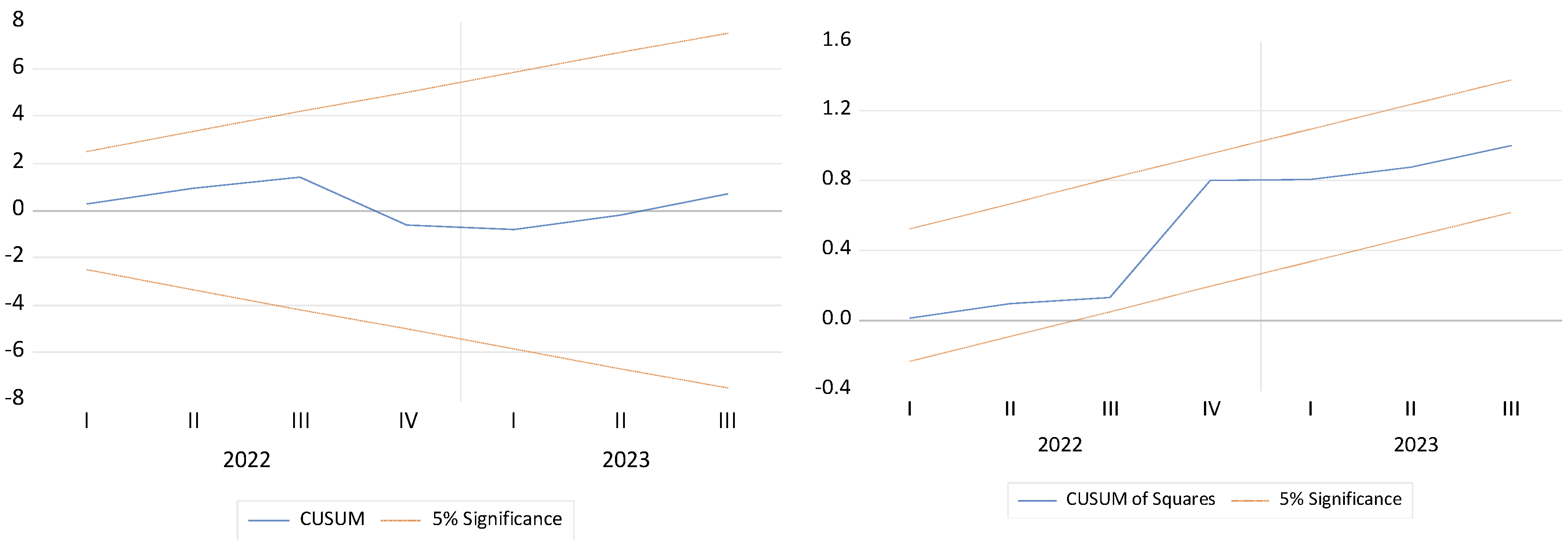
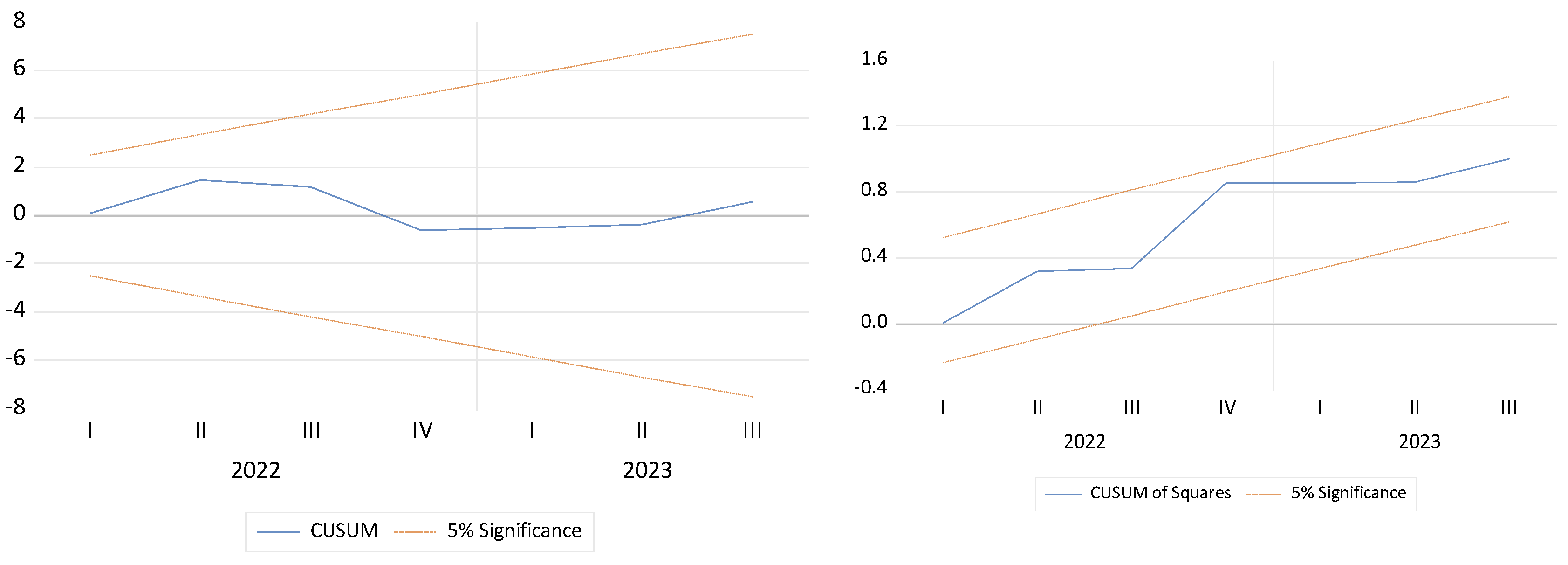
5.3. Robustness Checks

We check the robustness of the NARDL model by evaluating the stability of the estimated parameters. For that reason, we apply the cumulative sum of recursive residuals (CUSUM) and the CUSUM of squares (CUSUMSQ) tests, as proposed by Brown et al. (1975). CUSUM statistics and bands represent the bounds of the critical region for the test at the 5% significance level. If the cumulative sum goes outside the area between the two critical lines, the test finds parameter instability. Figure 4 and Figure 5 plot the results for the CUSUM and CUSUMSQ tests in the specifications of the unemployment gap and the output gap, respectively. The results show that in both specifications, the plots of the CUSUM and CUSUMSQ statistics stay within the critical bounds of the 5% confidence interval, implying the stability of the model.

Furthermore, the cumulative dynamic multipliers obtained from the NARDL models are plotted in Figure 6 and Figure 7. The asymmetry curve reflects the difference between the dynamic multiplier associated with positive and negative shocks to the explanatory variable. This curve is plotted along with its lower and upper bands at the 95% confidence interval to provide the statistical significance of the asymmetry at each horizon h. If the zero line falls within the lower and upper bands, the asymmetric effects of each explanatory variable are not statistically significant at the 5% level. The multiplier in Figure 6 shows the pattern of the inflation rate’s adjustment to its new long-run equilibrium in response to a negative or positive shock to the unemployment gap for a given 30-quarter horizon. The graph in this figure confirms that there is an inverse relationship between inflation and the unemployment gap in the short and long run. The response of inflation is significantly asymmetric, and it takes approximately 10 quarters for inflation to reach a new equilibrium. The behavior of the dynamic multiplier is consistent with the significant long-run asymmetry seen in the NARDL model.

The multiplier in Figure 7 shows the pattern of the inflation rate adjustment to its new long-run equilibrium in response to a negative or positive shock to the output gap at a given 30-quarter horizon. The graph confirms the existence of a positive relationship between inflation and the output gap, both in the short and long run, and that the response of inflation is significantly asymmetric. It takes about 12 quarters for inflation to reach a new equilibrium. The behavior of the dynamic multiplier is consistent with the presence of significant long-run and short-run asymmetry in the NARDL model. Also, Figure 6 and Figure 7 show that the inflation adjustment to the new long-run equilibrium following an output shock takes longer than adjustment after an unemployment shock.

6. Discussion of the Empirical Findings

This study investigates the asymmetries in the effects of the unemployment gap and the output gap on inflation in Greece by employing a nonlinear ARDL approach. The empirical results show a negative and asymmetric long-run relationship between inflation and the unemployment gap. Moreover, we find positive and asymmetric long-run and short-run relationships between inflation and the output gap. Our findings are consistent with previous studies that identified a nonlinear relationship between economic slack and inflation (Clark et al. 1996; Huh and Jang 2007; Baghli et al. 2007; Önder 2009; Granger and Jeon 2011; Xu et al. 2015; Kumar and Orrenius 2016; Donayre and Panovska 2016; Bildirici and Ozaksoy 2016, 2018; Lepetit 2020; Mihajlović and Marjanović 2020; Cristini and Ferri 2021; Pham and Sala 2022; Lahcen et al. 2022; Biçer and Burgac Cil 2023). In addition, in the long run, the results indicate that the positive shocks to the unemployment gap have a greater impact on inflation than negative shocks. In contrast, in the long run, the negative shocks to the output gap have a greater impact on inflation than positive shocks. According to the findings of both estimates, inflation tends to be more sensitive during recessions than during expansions. These findings are consistent with the studies of Pham and Sala (2022) and Lahcen et al. (2022). Also, recent empirical research (Inoue et al. 2024; Hobijn et al. 2023; Baba et al. 2023) indicates that the Phillips curve has started to steepen following the pandemic, even when using simpler models that previously suggested a “flatter” curve. This trend is observable in the US, the EU, and the OECD countries.

During the examined period, Greece experienced a severe and prolonged economic recession, accompanied by abnormally high unemployment rates. The country’s decade-long economic recession raised economic uncertainty and profoundly impacted consumer and business confidence. The expectation of falling prices caused delays in both purchases and investments. In his 2020 speech at the Economic Council, Philip Lane2 argued that asymmetric shocks, which have varying effects across member states of the Eurozone, complicate the process of making competitiveness adjustments within a monetary union when inflation remains low. This situation is exacerbated if a prolonged period of low inflation undermines inflation expectations. In such scenarios, the macroeconomic impact of negative shocks becomes more severe and long-lasting. Although the Greek economy began to grow steadily again after 2018, inflation remained low. The downturn in economic activity caused by the COVID-19 pandemic created new deflationary pressures, pushing inflation into negative territory. Consequently, the prolonged economic downturn in Greece followed by the implementation of stringent economic policies outlined in Greece’s memorandum, along with the heightened uncertainty triggered by the COVID-19 pandemic, had adverse effects on economic activity and imposed deflationary pressures on prices. These factors likely resulted in a stronger response to inflation during recessions than periods of economic recovery, as suggested by the study’s results.

It is important to note that the empirical findings presented in this paper are subject to certain limitations regarding the accuracy and reliability of the estimated unemployment and output gap. The accuracy of calculating the unemployment gap and the output gap depends heavily on the accuracy of estimating the NAIRU and potential output, which can be influenced by the filtering method used. Additionally, the relationships between the unemployment gap and inflation and between the output gap and inflation are only fully understood after the fact, making them less useful for forecasting inflation. Despite these limitations, understanding the characteristics of this relationship can still provide valuable insights for economic policymakers. As high inflation affects economic activities and creates uncertainty, flexibility policies are important in terms of enabling the economy to achieve higher output and employment levels and lower price levels.

7. Conclusions

This paper uses Greek quarterly macroeconomic data from 1998 to 2023 to investigate differences in the way the economy behaves at different stages of the business cycle. The analysis presented in this paper uses a nonlinear ARDL approach that is based on the Phillips curve. It has been argued that asymmetries in the business cycle have significant implications for economic theory, modeling, and policymaking. The findings from the Greek economy shed light on the dynamics between inflation with the unemployment gap and the output gap, highlighting the varying sensitivity of inflation to different phases of the business cycle. Specifically, the results indicate the existence of an inverse asymmetric relationship between inflation and the unemployment gap, but this relationship is only observed in the long run. Additionally, the results reveal the existence of a similar asymmetric relationship between inflation and the output gap in both the long and short run. In the long run, inflation appears to be more sensitive to periods of economic recession than expansion, while in the short run, inflation tends to rise and exhibit greater sensitivity during economic expansions. In conclusion, the Phillips curve is still evident in the Greek economy, but its nonlinearities raise serious challenges in relation to monetary policy implementation. Therefore, the Phillips curve remains a significant framework for comprehending the cyclical interactions between inflation and economic activity.

The global economy has faced significant negative supply shocks in the last few decades, affecting output, unemployment, and inflation. This complexity makes it challenging for monetary policy to navigate the trade-offs between output, unemployment, and inflation and face the asymmetric risks. Policymakers must consider two critical questions: the source of the economic shocks and how long they are likely to persist for. This assessment is particularly important because shocks impact both demand and supply, making it more difficult to identify the primary drivers of inflation. Inflation was primarily driven by rising energy costs and persistent supply-side constraints during the energy crisis. On the other hand, inflation, following the reopening of the economy after the pandemic’s crisis phase, was mainly fueled by a surge in demand. Therefore, policymakers must understand the underlying causes of these ongoing shocks, as this knowledge is crucial for developing an appropriate policy response. If supply shocks are the dominant source of inflation, monetary policy should intervene if these shocks continue to keep inflation expectations stable and prevent inflation from becoming ingrained. Conversely, it should respond swiftly to demand shocks that could push medium-term inflation above the desired target.

As a member of the Eurozone, Greece lacks monetary sovereignty, which restricts its ability to implement monetary policy measures. However, Greece should continue to reform its labor market, which would help remove supply-side distortions and improve productivity. Given Greece’s high debt-to-GDP ratio, prioritizing supply-side reforms is crucial for reducing unemployment and achieving sustainable growth. According to Pissarides (2013), these reforms can accelerate the growth of productivity, reduce real marginal costs, and ease upward inflationary pressure. If Greece had adopted an alternative fiscal policy—such as lowering income taxes or increasing public investment, both financed by a reduction in public consumption spending—and if product market reforms had been implemented more swiftly and effectively while the political system had cooperated in enacting the necessary measures to overcome the crisis—as was the case in Portugal and Ireland—these changes could have significantly improved the situation (Economides and Philippopoulos 2022). In future research, we aim to analyze fiscal policy in Greece, particularly in light of the substantial austerity measures enacted following the onset of the economic crisis.

References

1. Abid, Mehdi, Mohammed Benmeriem, Zouheyr Gheraia, Habib Sekrafi, Hanane Abdelli, and Abdelhadi Meddah. 2023. Asymmetric effects of economy on unemployment in Algeria: Evidence from a nonlinear ARDL approach. Cogent Economics & Finance 11: 2192454. [Google Scholar] [CrossRef]
2. Ahn, JaeBin, and Jiwon Lee. 2023. The Role of Import Prices in Flattening the Phillips Curve: Evidence from Korea. Journal of Asian Economics 86: 101605. [Google Scholar] [CrossRef]
3. Akaike, Hirotugu. 1974. A new look at the statistical model identification. IEEE Transactions on Automatic Control 19: 716–23. [Google Scholar] [CrossRef]
4. Al-Nassar, Nassar S., and Abdulrahman A. Albahouth. 2023. Inflation Spillovers among Advanced and Emerging Economies: Evidence from the G20 Group. Economies 11: 126. [Google Scholar] [CrossRef]
5. Ascari, Guido, and Luca Fosso. 2021. The Inflation Rate Disconnect Puzzle: On the International Component of Trend Inflation and the Flattening of the Phillips Curve. Norges Bank Working Papers. Available online: https://ssrn.com/abstract=3999368 (accessed on 10 September 2024).
6. Baba, Chikako, Mr Romain A. Duval, Romain Duval, Ting Lan, and Petia Topalova. 2023. The 2020–2022 Inflation Surge Across Europe: A Phillips-Curve-Based Dissection. IMF Working Paper, No. 2023/030. Bretton Woods: International Monetary Fund. [Google Scholar]
7. Baghli, Mustapha, Christophe Cahn, and Henri Fraisse. 2007. Is the inflation–output Nexus asymmetric in the Euro area? Economics Letters 94: 1–6. [Google Scholar] [CrossRef]
8. Ball, Laurence M., and Sandeep Mazumder. 2011. Inflation Dynamics and the Great Recession. NBER Working Paper No. w17044. Available online: https://ssrn.com/abstract=1841281 (accessed on 10 August 2024).
9. Ball, Laurence M., Gita Gopinath, Daniel Leigh, Prachi Mishra, and Antonio Spilimbergo. 2021. US Inflation: Set for Takeoff? Voxeu.org. CEPR Policy Portal 7. Available online: https://cepr.org/voxeu/columns/us-inflation-set-take (accessed on 10 August 2024).
10. Benigno, Pierpaolo, and Gauti B. Eggertsson. 2023. It’s Baaack: The Surge in Inflation in the 2020s and the Return of the Non-Linear Phillips Curve. Cambridge, MA: National Bureau of Economic Research, p. w31197. [Google Scholar] [CrossRef]
11. Biçer, Burhan, and Almila Burgac Cil. 2023. Symmetric and Asymmetric Dynamics of Output Gap and Inflation Relation for Turkish Economy. Prague Economic Papers 32: 520–49. [Google Scholar] [CrossRef]
12. Bildirici, Melike, and Fulya Ozaksoy. 2016. Non-linear analysis of post Keynesian Phillips curve in Canada labor market. Procedia Economics and Finance 38: 368–77. [Google Scholar] [CrossRef]
13. Bildirici, Melike, and Fulya Ozaksoy. 2018. Backward bending structure of Phillips curve in Japan, France, Turkey and the U.S.A. Economic Research 31: 537–49. [Google Scholar] [CrossRef]
14. Blanchard, Olivier, Eugenio Cerutti, and Lawrence Summers. 2015. Inflation and Activity: Two Explorations and Their Monetary Policy Implications. ECB Forum on Central Banking. Cambridge, MA: National Bureau of Economic Research. [Google Scholar]
15. Boehm, Christoph E., and Nitya Pandalai-Nayar. 2022. Convex Supply Curves. American Economic Review 112: 3941–69. [Google Scholar] [CrossRef]
16. Broock, William A., José Alexandre Scheinkman, W. Davis Dechert, and Blake LeBaron. 1996. A test for independence based on the correlation dimension. Econometric Reviews 15: 197–235. [Google Scholar] [CrossRef]
17. Brown, Robert L., James Durbin, and James M. Evans. 1975. Techniques for testing the constancy of regression relationships over time. Journal of the Royal Statistical Society Series B: Statistical Methodology 37: 149–92. [Google Scholar] [CrossRef]
18. Caballero, Ricardo J., and Mohamad Hammour. 1994. The cleansing effect of recession. American Economic Review 84: 1350–68. [Google Scholar]
19. Ciccarelli, Matteo, and Benoit Mojon. 2010. Global Inflation. The Review of Economics and Statistics 92: 524–35. [Google Scholar] [CrossRef]
20. Clark, Peter, Douglas Laxton, and David Rose. 1996. Asymmetry in the US output-inflation nexus. IMF Staff Papers 43: 216–51. [Google Scholar] [CrossRef]
21. Coibion, Olivier, and Yuriy Gorodnichenko. 2015. Is the Phillips Curve Alive and Well after All? Inflation Expectations and the Missing Disinflation. American Economic Journal: Macroeconomics 7: 197–232. [Google Scholar] [CrossRef]
22. Cristini, Annalisa, and Piero Ferri. 2021. Nonlinear models of the Phillips curve. Journal of Evolutionary Economics 31: 1129–55. [Google Scholar] [CrossRef]
23. Del Negro, Marco, Michele Lenza, Giorgio E. Primiceri, and Andrea Tambalotti. 2020. What’s Up with the Phillips Curve? NBER Working Paper No. 27003. Cambridge, MA: National Bureau of Economic Research. [Google Scholar]
24. Dickey, David A., and Wayne A. Fuller. 1979. Distributions of the estimators for autoregressive time series with a unit root. Journal of American Statistical Association 74: 427–31. [Google Scholar]
25. Dickey, David A., and Wayne A. Fuller. 1981. Likelihood ratio statistics for autoregressive time series with a unit root. Econometrica 49: 1057–72. [Google Scholar] [CrossRef]
26. Dixon, Huw. 1988. Controversy: The macroeconomics of unemployment in the OECD. The Economic Journal 108: 779–81. [Google Scholar] [CrossRef]
27. Donayre, Luiggi, and Irina Panovska. 2016. Nonlinearities in the U.S. wage Phillips Curve. Journal of Macroeconomics 48: 19–43. [Google Scholar] [CrossRef]
28. Economides, George, and Apostolis Philippopoulos. 2022. What Is Next? Public Debt and Economic Growth in Greece. CESifo Forum. Munich: Ifo Institute—Leibniz Institute for Economic Research at the University of Munich, vol. 23, pp. 24–29. [Google Scholar]
29. Economides, George, Dimitris Papageorgiou, and Apostolis Philippopoulos. 2021. Austerity, Assistance and Institutions: Lessons from the Greek Sovereign Debt Crisis. Open Economies Review 32: 435–78. [Google Scholar] [CrossRef]
30. Forbes, Kristin J., Joseph Gagnon, and Christopher G. Collins. 2021. Pandemic Inflation and Nonlinear, Global Phillips Curves. Voxeu.org. CEPR Policy Portal 21. Available online: https://voxeu.org/article/pandemic-inflation-and-nonlinear-global-phillips-curves (accessed on 19 August 2024).
31. Friedman, Milton. 1968. The Role of Monetary Policy. American Economic Review 58: 1–17. [Google Scholar]
32. Gagnon, Joseph, and Madi Sarsenbayev. 2022. 25 Years of Excess Unemployment in Advanced Economies: Lessons for Monetary Policy. Working Paper Series WP22-17. Washington, DC: Peterson Institute for International Economics. [Google Scholar]
33. Granger, Clive W. J., and Yongil Jeon. 2011. The evolution of the Phillips curve: A modern time series viewpoint. Economica 78: 51–66. [Google Scholar] [CrossRef]
34. Gross, Marco, and Willi Semmler. 2019. Mind the output gap: The disconnect of growth and inflation during recessions and convex phillips curves in the euro area. Oxford Bulletin of Economics and Statistics 81: 817–48. [Google Scholar] [CrossRef]
35. Gürkaynak, Refet S., Andrew Levin, and Eric Swanson. 2010. Targeting anchor long-run inflation expectations? evidence from long-term bond yields in the U.S., U.K., and Sweden. Journal of the European Economic Association 8: 1208–42. [Google Scholar]
36. Harding, Martín, Jesper Lindé, and Mathias Trabandt. 2023. Understanding Post-COVID Inflation Dynamics. Journal of Monetary Economics 140: 101–18. [Google Scholar] [CrossRef]
37. Haschka, Rouven E. 2024. Examining the New Keynesian Phillips Curve in the U.S.: Why has the relationship between inflation and unemployment weakened? Research in Economics 78: 100987. [Google Scholar] [CrossRef]
38. Hindrayanto, Irma, Anna Samarina, and Irina M. Stanga. 2019. Is the Phillips curve still alive? Evidence from the euro area. Economics Letters 174: 149–52. [Google Scholar] [CrossRef]
39. Hobijn, Bart, Russell Miles, James Royal, and Jing Zhang. 2023. The Recent Steepening of Phillips Curves. Chicago Fed Letter 475. Available online: https://www.chicagofed.org/publications/chicago-fed-letter/2023/475 (accessed on 11 December 2024). [CrossRef]
40. Hodrick, Robert J., and Edward C. Prescott. 1997. Business Cycles: An Empirical Investigation. Journal of Money, Credit and Banking 29: 1–16. [Google Scholar] [CrossRef]
41. Huh, Hyeon-seung, and Inwon Jang. 2007. Nonlinear Phillips curve, sacrifice ratio, and the natural rate of unemployment. Economic Modelling 24: 797–813. [Google Scholar] [CrossRef]
42. Inoue, Atsushi, Barbara Rossi, and Yiru Wang. 2024. Has the Phillips Curve Flattened? CEPR Discussion Paper, No. 18846. London: Centre for Economic Policy Research. [Google Scholar]
43. International Monetary Fund. 2013. The Dog that Didn’t bark: Has Inflation Been Muzzled or Was It Just Sleeping? In World Economic Outlook: Hopes, Realities, Risks. Bretton Woods: International Monetary Fund, pp. 79–96. [Google Scholar]
44. Jašová, Martina, Richhild Moessner, and Előd Takáts. 2018. Domestic and global output gaps as inflation drivers: What does the Phillips curve tell? Economic Modelling 87: 238–53. [Google Scholar] [CrossRef]
45. Jorgensen, Peter Lihn, and Kevin J. Lansing. 2024. Anchored Inflation Expectations and the Slope of the Phillips Curve. Federal Reserve Bank of San Francisco Working Paper No. 2019–27. San Francisco: Federal Reserve Bank of San Francisco. [Google Scholar]
46. Kumar, Anil, and Pia M. Orrenius. 2016. A closer look at the Phillips curve using state-level data. Journal of Macroeconomics 47: 84–102. [Google Scholar] [CrossRef]
47. Lahcen, Mohammed Ait, Garth Baughman, Stanislav Rabinovich, and Hugo van Buggenum. 2022. Nonlinear unemployment effects of the inflation tax. European Economic Review 148: 104247. [Google Scholar] [CrossRef]
48. Laxton, Douglas, David Rose, and Demosthenes Tambakis. 1999. The U.S. Phillips curve: The case for asymmetry. Journal of Economic Dynamics and Control 23: 1459–85. [Google Scholar] [CrossRef]
49. Lepetit, Antoine. 2020. Asymmetric unemployment fluctuations and monetary policy trade-offs. Review of Economic Dynamics 36: 29–45. [Google Scholar] [CrossRef]
50. Li, Youshu, and Junjie Guo. 2022. The asymmetric impacts of oil price and shocks on inflation in BRICS: A multiple threshold nonlinear ARDL model. Applied Economics 54: 1377–95. [Google Scholar] [CrossRef]
51. Lucas, Robert E. 1973. Some International Evidence on Output-Inflation Trade-offs. American Economic Review 63: 326–34. [Google Scholar]
52. MacKinnon, James. 1996. Numerical Distribution Functions for Unit Root and Cointegration Tests. Journal of Applied Econometrics 11: 601–18. [Google Scholar] [CrossRef]
53. Macklem, Tiff. 1997. Capacity constraints, price adjustment, and monetary policy. Bank of Canada Review 1997: 39–56. [Google Scholar]
54. McLeay, Michael, and Silvana Tenreyro. 2020. Optimal inflation and the identification of the Phillips Curve. The University of Chicago Press Journals 34: 199–255. [Google Scholar] [CrossRef]
55. Mihajlović, Vladimir, and Gordana Marjanović. 2020. Asymmetries in effects of domestic inflation drivers in the Baltic States: A Phillips curve-based nonlinear ARDL approach. Baltic Journal of Economics 20: 94–116. [Google Scholar] [CrossRef]
56. Narayan, Paresh Kumar. 2005. The saving and investment nexus for China: Evidence from cointegration tests. Applied Economics 37: 1979–90. [Google Scholar] [CrossRef]
57. Newey, Whitney K., and Kenneth D. West. 1994. Automatic lag selection in covariance matrix estimation. Review of Economic Studies 61: 631–53. [Google Scholar] [CrossRef]
58. OECD Statistics. 2024. Available online: https://data.oecd.org/ (accessed on 1 August 2024).
59. Orphanides, Athanasios, and John C. Williams. 2005. Inflation scares and forecast-based monetary policy. Review of Economic Dynamics 8: 498–527. [Google Scholar] [CrossRef]
60. Önder, A. Özlem. 2009. The stability of the Turkish Phillips curve and alternative regime shifting models. Applied Economics 41: 2597–604. [Google Scholar] [CrossRef]
61. Passamani, Giuliana, Alessandro Sardone, and Roberto Tamborini. 2022. Inflation puzzles, the Phillips Curve and output expectations: New perspectives from the Euro Zone. Empirica 49: 123–53. [Google Scholar] [CrossRef]
62. Pesaran, M. Hashem, Yongcheol Shin, and Richard J. Smith. 2001. Bounds testing approaches to the analysis of level relationships. Journal of Applied Econometrics 16: 289–326. [Google Scholar] [CrossRef]
63. Pham, Binh Thai, and Hector Sala. 2022. Cross-country connectedness in inflation and unemployment: Measurement and macroeconomic consequences. Empirical Economics 62: 1123–46. [Google Scholar] [CrossRef] [PubMed]
64. Phelps, Edmund S. 1967. Phillips Curves, Expectations of Inflation and Optimal Unemployment Over Time. Economica 34: 254–81. [Google Scholar] [CrossRef]
65. Phillips, Alban W. 1958. The Relation between Unemployment and the Rate of Change of Money Wage Rates in the United Kingdom, 1861–957. Economica 25: 283–99. [Google Scholar]
66. Phillips, Peter C., and Pierre Perron. 1988. Testing for a unit root in time series regression. Biometrika 75: 335–46. [Google Scholar] [CrossRef]
67. Pissarides, Christopher A. 2000. Equilibrium Unemployment Theory. Cambridge, MA: MIT Press. [Google Scholar]
68. Pissarides, Christopher A. 2013. Unemployment in the great recession. Economica 80: 385–403. [Google Scholar] [CrossRef]
69. Ratner, David, and Jae Sim. 2022. Who Killed the Phillips Curve? A Murder Mystery; Board of Governors of the Federal Reserve System Working Paper, No. 2022–28; Washington, DC: Board of Governors of the Federal Reserve System.
70. Rudd, Jeremy, and Karl Whelan. 2007. Modeling Inflation Dynamics: A Critical Review of Recent Research. Journal of Money, Credit and Banking 39: 155–70. [Google Scholar] [CrossRef]
71. Samuelson, Paul A., and Robert M. Solow. 1960. Analytical Aspects of Anti-Inflation Policy. American Economic Review 50: 177–94. [Google Scholar]
72. Shin, Yongcheol, Byungchul Yu, and Matthew Greenwood-Nimmo. 2014. Modelling asymmetric cointegration and dynamic multipliers in a nonlinear ARDL framework. In The Festschrift in Honor of Peter Schmidt: Econometric Methods and Applications. Edited by Robin C. Sickles and William C. Horrace. New York: Springer, pp. 281–314. [Google Scholar]
73. Tang, Bo, and Carlos Bethencourt. 2017. Asymmetric unemployment-output tradeoff in the Eurozone. Journal of Policy Modeling 39: 461–81. [Google Scholar] [CrossRef]
74. Xu, Qifa, Xufeng Niu, Cuixia Jiang, and Xue Huang. 2015. The Phillips Curve in the US: A nonlinear quantile regression approach. Economic Modelling 49: 186–97. [Google Scholar] [CrossRef]
Figure 1. Inflation, GDP, and unemployment rate in Greece. Note: author’s calculations; GDP is in millions of euros (constant 2015).
Economies 12 00346 g001aEconomies 12 00346 g001b
Figure 2. A graph of the estimated unemployment gap. Note: author’s calculations; the cycle denotes the unemployment gap.
Economies 12 00346 g002
Figure 3. A graph of the estimated output gap. Note: author’s calculations; cycle denotes the output gap.
Economies 12 00346 g003
Figure 4. A plot of CUSUM and CUSUMSQ tests with the unemployment gap as the explanatory variable. Note: author’s calculations.
Economies 12 00346 g004
Figure 5. A plot of CUSUM and CUSUMSQ tests with the output gap as the explanatory variable. Note: author’s calculations.
Economies 12 00346 g005
Figure 6. Dynamic multiplier impact of unemployment shocks on inflation. Note: author’s calculations.
Economies 12 00346 g006
Figure 7. Dynamic multiplier impact of output shocks on inflation. Note: author’s calculations.
Economies 12 00346 g007