An Empirical Study of the Impact of the Euro on Cross-Country Diversification

Abstract

The euro was launched, on 1 January 1999, as a common currency for members of the European Union that complied with the Maastricht Treaty. The Maastricht Treaty calls for the coordination of major macroeconomic policies, such as inflation, budget balance, public debt, and long-term interest rates. Theoretically, the coordination of these policy issues and the launch of a common currency will increase the degree of market integration among member countries. This paper empirically tests the impact of the euro on the degree of market integration by looking at the comovement of the European equity markets and a sample of OECD equity markets. Weekly stock market indices for the period covering seven years before the euro and seven years after the euro was implemented was used. The results show that cross-country divergences in stock markets continued after the euro. There is no evidence of cointegration after the adoption of the euro. Cross-country portfolio diversification continues to be beneficial even among euro countries.

1. Introduction

The euro was launched, on 1 January 1999, by eleven1 of the European Union member countries. The launch of the euro was just one step in a series of negotiations and treaties among EU member countries to achieve an economic and political union. Even before the launch of the euro, significant macroeconomic policies had been coordinated. The euro started circulating in the form of coins and bills on 1 January 2002. The European Central Bank (ECB) manages European monetary policy independently of political authorities. As of 1 January 1999, member countries have been required to comply with the convergence criteria set in the 1993 Maastricht Treaty, which include the following: price stability such that the inflation rate does not exceed 1.5 percent above the rate for the three member states with the lowest inflation rates; budget deficit not exceeding three percent of GDP; government debt not exceeding 60 percent of GDP; long-term interest rates maintained within two percentage points of the three best-performing members; and the exchange rates within a band established by the European Monetary System.

Starting on 1 January 1999, the exchange rates between the member countries’ currencies and the euro were fixed. The prices of goods and services were quoted in euros. Government debt and foreign exchange were denominated in euros. The flow of goods, labor, and capital among member countries was already liberalized.

There are two theoretical views regarding the impact of policy coordination on capital market integration and global diversification. The first view is that policy coordination leads to the greater integration of country markets and the convergence of performances such that cross-country diversification benefits would be lost. Halpern (1993) argues that correlations among stock markets increase and cross-country diversification benefits become less obvious as macroeconomic policies are coordinated. Consistent with this notion and regional economic blocks, Heaney et al. (2002) find that markets are segmented on a regional basis2.

The second view is that local economic factors, such as the labor force, may not respond to macroeconomic policy changes due to cultural and linguistic reasons. In addition to this, Bekaert and Harvey (1995) argue that the mixture of industries in various countries is different and, hence, they react differently to macroeconomic policy changes. In fact, Steeley et al. (1998) found that cointegration relationships among European markets decreased after the relaxation of exchange controls in the 1970s and 1980s. The implication of these findings is that macroeconomic policy coordination does not necessarily result in capital market integration. Further, the drive for cross-country diversification should not be abandoned. There are some investment analysts and strategists who argue along the same lines using factual evidence from European markets following the launch of the euro3.

How effective has the launch of the euro been at integrating European equity markets? This is an empirical question. Therefore, the purpose of this study was to estimate and analyze the impact of the euro on European capital markets integration and cross-country diversification of investments. The launch of the euro and the enforcement of the various macroeconomic policies in Europe are so significant that an investigation is warranted. To what extent have the eurozone countries complied with the convergence criteria? An overview of some macroeconomic figures is also provided. This paper analyzes the changes in correlations and cointegration among the twelve eurozone countries, using 7 years of pre-euro and 7 years of post-euro weekly national stock market indices. Further, the mean-variance framework4 is used to check to what extent diversification opportunities changed after the euro. Analyses of some non-euro developed countries are provided for comparison purposes. While there is an abundance of literature on capital market integration, there has been no empirical test of the European market since the adoption of the euro5.

The paper is organized as follows: Section 2 presents a review of the literature, Section 3 describes the methodology and the data, Section 4 presents the empirical results, Section 5 discusses the results, and, finally, Section 6 concludes the study.

2. Literature Review

Most of the previous studies did not find significant cointegration among markets. Chan et al. (1992) analyzed stock prices in the US, Japan, South Korea, Taiwan, Hong Kong, and Singapore and found that these markets were weak-form efficient but not cointegrated among themselves. DeFusco et al. (1996) performed cointegration tests on weekly stock indices of 13 emerging markets and the US market. They found no significant cointegration relationships among the markets. Steeley et al. (1998) examined the effect of the removal of exchange controls in several European countries on the comovement of their stock market indices using cointegration techniques. Most of the exchange control removals took place in the 1970s and 1980s for the countries in their sample (France, Switzerland, Italy, Germany, and the UK). They used monthly price index data. Their results show that the cointegration relationships disappeared after the relaxation of exchange controls for all countries in the sample, except the UK. For the UK, there was no cointegration relationship even before exchange control removals.

One possible reason for the lack of cointegration in these studies is that local economic factors do not necessarily respond to changes in economic policies. Even if some sectors respond, there is a “home bias” in institutional decision making, as evidenced by Buch (2000) among German banks. The above studies indicate that the national markets for which cointegration relationships decreased or disappeared gained in terms of market efficiency.

Beliu and Higgins (2004) applied fractional cointegration and found convergence between inflation and interest rates but no convergence among outputs. A more recent study by Umutlu et al. (2023) compared cross-country and cross-industry market integrations and concluded that industry indices are more segmented than country indices. Hence, cross-industry diversification can result in greater risk-reduction benefits.

On the other hand, Steeley and Steeley (1999) conducted a study of European stock market responses to shocks in other European markets and found that the impulse response of all markets in the study (France, Switzerland, Germany, Spain, Italy, and the UK) increased after the liberalization of exchange controls and coordination of other macroeconomic policies. These liberalizations took place in the countries in the late 1970s and early 1980s, except for Spain, which had exchange controls until 1992. They also report an increase in the cross-correlations of these markets after liberalization and state that a substantial portion of the increase in correlations resulted from exchange control liberalization than other macroeconomic policy changes.

Heaney et al. (1999, 2002) found that market integration is regionally clustered. This means the degree of integration of national markets increases with geographical proximity and regional economic blocks. For example, the Indonesian stock market would be more integrated with the Malaysian stock market, and the Peruvian stock market would be more integrated with the Brazilian stock market. The European markets belong to the same geographic region and the same economic block, which indicates a greater integration of their markets than with other markets outside the European Union.

Aggarwal and Kyaw (2005) tested the cointegration of the equity markets of the US, Canada, and Mexico around the passage of NAFTA (in 1993). They found that the stock returns were stationary, but there was no evidence of cointegration during the pre-NAFTA period. Post-NAFTA, they found some evidence of cointegration among the three markets.

Barunik and Vacha (2013) studied contagion among the Central and the Eastern European (CEE) stock markets during the financial crisis. They found a lower degree of contagion between the Central and Eastern European stock market indices and the German DAX after the stock market crash of 2008. Likewise, Cărăuşu et al. (2018), in their study of contagion between the Central and East European (CEE) and the Western European and US capital markets, between 2000 and 2016, found evidence of contagion of the CEE stock markets between 2005 and 2009, but they found evidence of de-contagion from 2010 to 2016 of the stock markets of Bulgaria, Hungary, the Czech Republic, and Poland to the US stock market. Pardal et al. (2020) cite Krarup (2021), who argues that the case of European capital markets integration is an epidemic problem, in which there is strong uncertainty concerning the interpretation of relevant standard doctrines. They further quote Krarup (2021) and Bremus and Kliatskova (2020), who also draw attention to this problem by analyzing the harmonization and convergence, in the form of institutional quality, of the European capital markets.

The extant literature presented above shows no or little evidence of stock market cointegration. Although the increase in correlations and the advents of globalization and regional economic integrations imply the increased comovement of stock markets, the powerful cointegration tests show little support for this view. This paper presents analyses of European equity market integration and correlation around the launch of the euro and evaluates the euro’s impact on the cross-country diversification of portfolio investment.

3. Methodology and Data

The correlation between two market indices indicates the extent to which the two markets move together. A simple correlation can be used to see the impact of policy change on the cointegration of markets. An increase in the correlation indicates an increase in cointegration and a decrease in cross-country diversification opportunities. Bekaert and Harvey (1995) argue that although a correlation coefficient has been used as a measure of capital market integration in some studies, it is not dependable because the mix of industries in various countries may differ, which can cause a low or negative correlation with other countries. They show that the degree of capital market integration varies over time, and for integrated markets, stock returns tend to depend more on common global factors and less on local factors. Halpern (1993) states that the correlation between any two markets is influenced by the markets’ volatility and transactions costs. High volatility and low transaction costs increase arbitrage activities and, hence, correlation between the markets. The pricing of specific risk factors will converge with a reduction in transaction costs. If business risks differ among local markets, however, capital market returns will continue to diverge, and the diversification benefits from cross-country investment will be preserved.

A stronger analysis of the comovement of stock markets is obtained using the cointegration technique. For two variables, x and y, to be cointegrated, they have to be integrated of the same order (such as unit root), and a linear combination of them should be stationary.

y_t = α + βx_t + u_t

(1)

y_t = α + γt + βx_t + u_t

(2)

Equation (1) is without a trend, and Equation (2) is with a trend. Both equations have constants. A cointegration test is based on the residuals from the above regressions.

∆û_t = δû_t-1 + Σθ_j∆û_t-j + ε_t j = 1, 2, 3, …., P

(3)

The lag length P is usually determined using the Akaike information criteria (AIC). The test for cointegration is based on δ. The test statistic is the t-test (δ = 0), and if there is no lag term, also the z-test (N*δ). Significant negative test statistics suggest the rejection of the unit root and evidence of cointegration6.

Several studies have tested the cointegration between two variables or among several variables using this technique although the exact model specifications may differ. For more than two variables, the equation becomes a multiple regression equation.

Weekly Data Stream total market indices adjusted for dividends and stock splits were used in this study7. These indices are based on the US dollar. The uniformity in index construction and the measurement in US dollars are useful in that there is no need to include an exchange rate variable in the analysis. For each of the countries in the study, the stock market index values were obtained for the period of January 1992 through December 2005, which covers the seven years before and the seven years after the launch of the euro. Weekly index returns were calculated as a percentage change in the index value over the previous week. Other macroeconomic data, such as the GDP growth rate, inflation rate, interest rate, public debt as a percent of GDP, budget balance as a percent of GDP, and unemployment rate, were obtained on an annual basis from the Data Stream database. The countries included in the study are the twelve eurozone countries (Austria, Belgium, Finland, France, Germany, Greece, Ireland, Italy, Luxembourg, the Netherlands, Portugal, and Spain) and ten non-euro OECD countries (Australia, Canada, Denmark, Japan, New Zealand, Norway, Sweden, Switzerland, the UK, and the US) for comparison. The world market index is also included to analyze any possible change in each country’s market relative to the world market.

4. Empirical Results

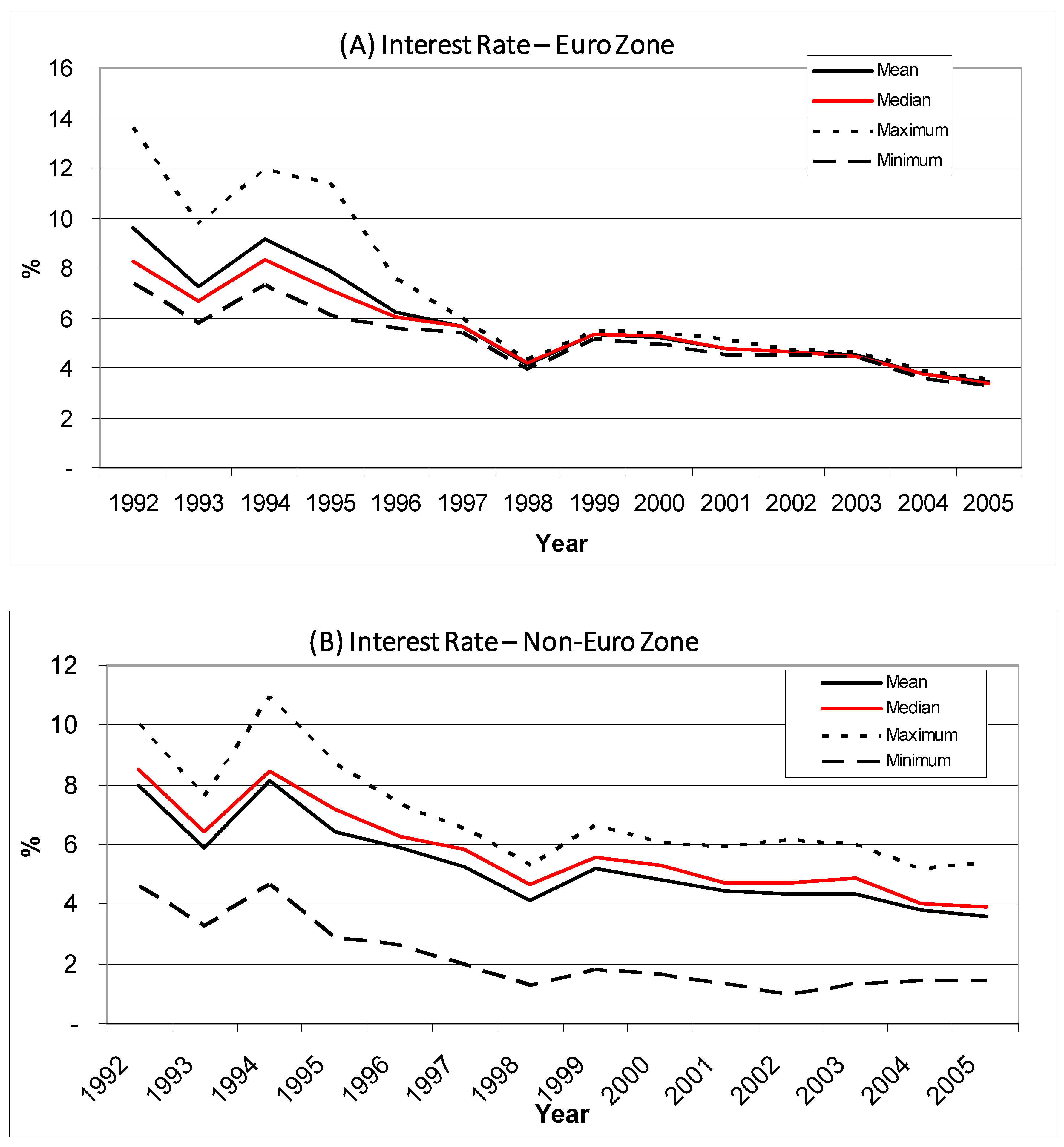
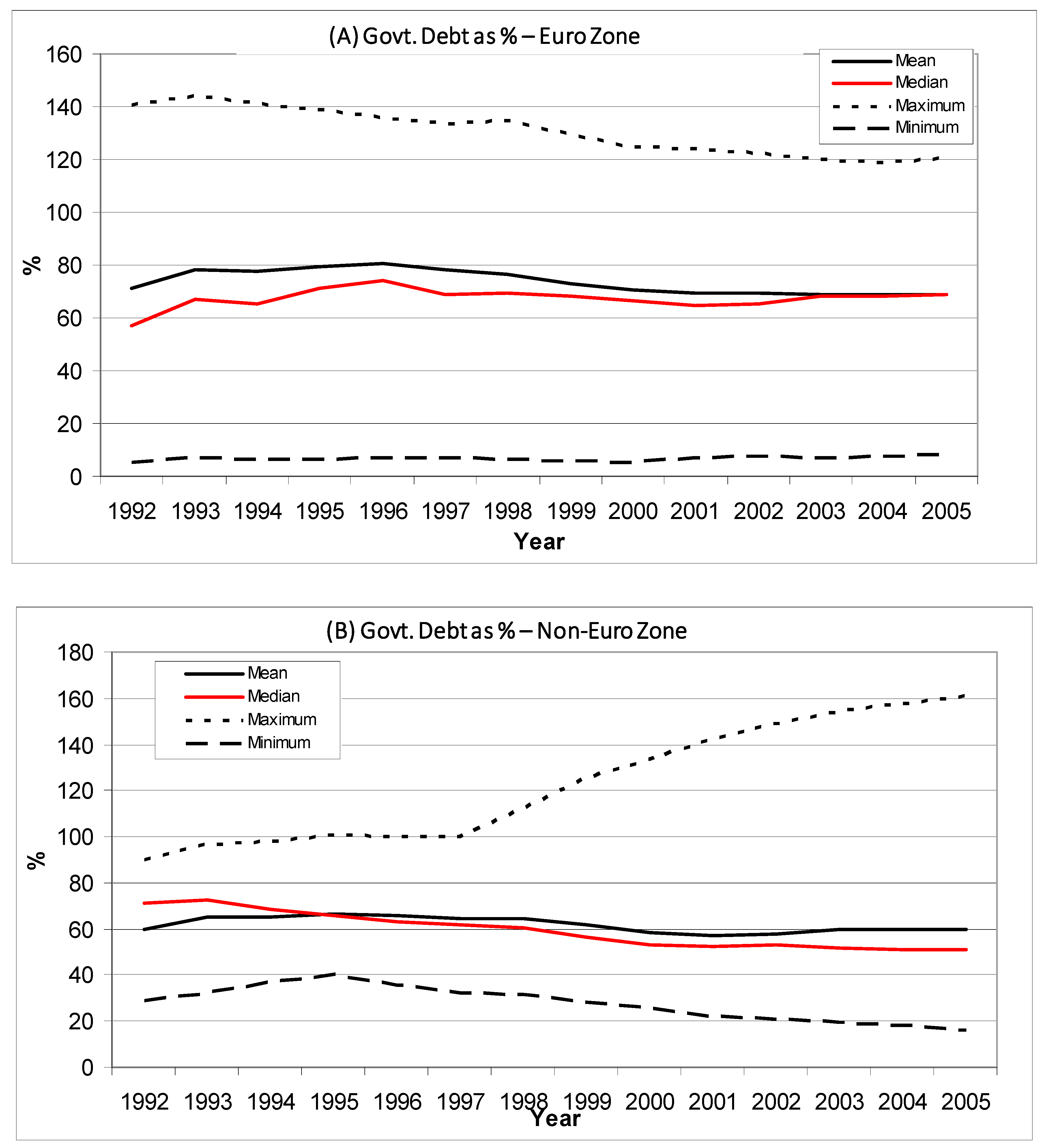
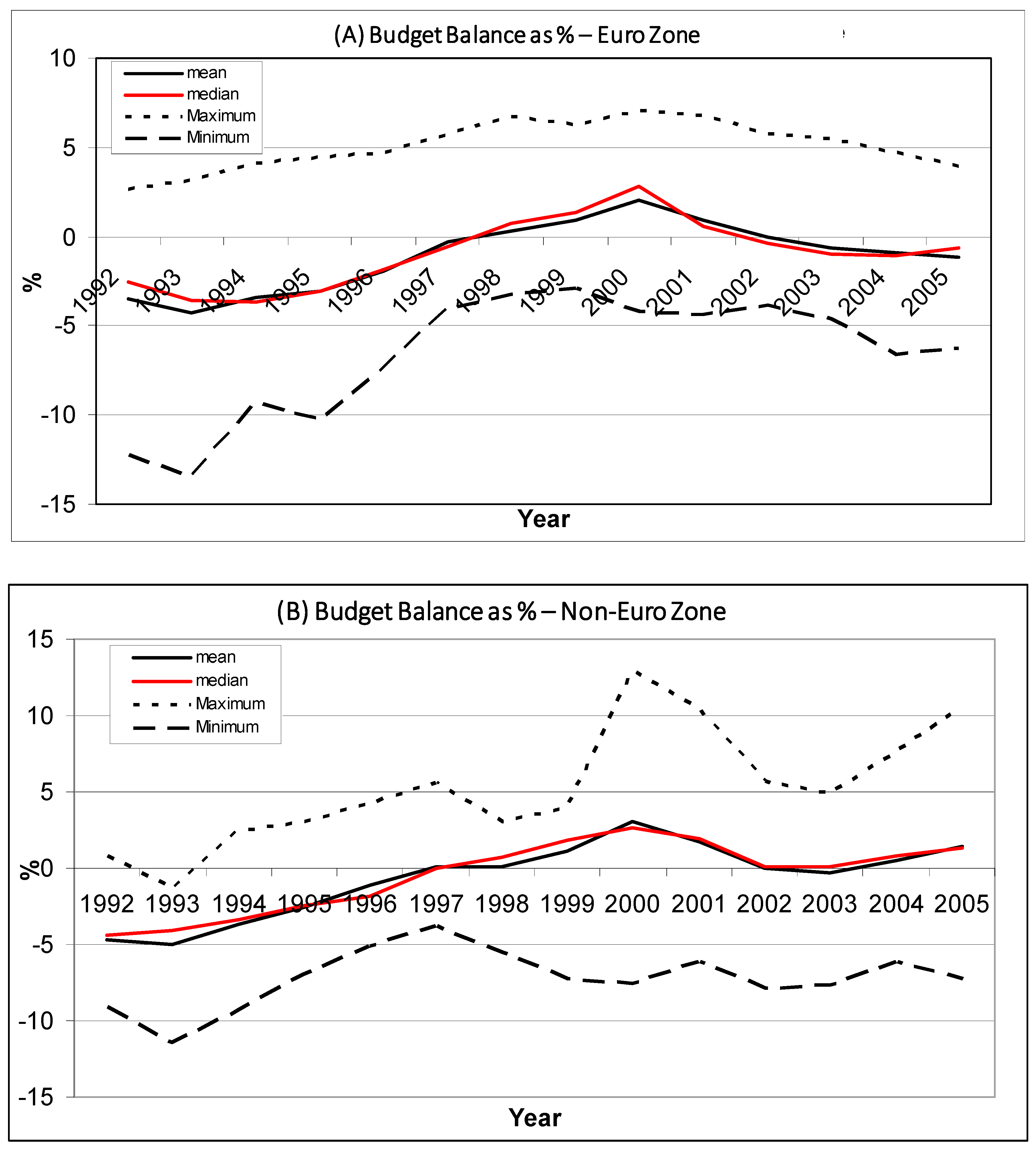
4.1. Preliminary Description

Table 1. Descriptive statistics stock index returns.

Panel A: 13 January 1992–19 December 2005.
The returns are based on Data Stream country total return market indices. The returns are measured weekly and expressed in percent. Autocorrelation functions (ACFs) of the index returns for up to 6 lags are reported. * ACF coefficient indicating significance at the 5% level. All mean returns are significant at the 5% level, except for Japan’s index return. The number of observations is 728 for all countries covering the weeks from 13 January 1992 to 19 December 2005.
	Mean	Median	Std. Deviation	Minimum	Maximum	Kurtosis	Skew-ness	ACF Coefficients for Lags
								1	2	3	4	5	6
Austria	0.211	0.279	1.855	−6.711	6.851	0.968	−0.097	0.085 *	0.098 *	0.031 *	0.083 *	0.038 *	−0.048 *
Belgium	0.248	0.383	2.258	−10.672	13.485	5.14	−0.070	−0.061	0.011	0.034	0.003	−0.059	0.029
Finland	0.508	0.529	4.607	−19.272	15.488	1.524	−0.188	−0.012	0.033	0.047	−0.005	0.135 *	0.015 *
France	0.256	0.386	2.696	−11.791	10.867	1.853	−0.253	−0.102 *	0.007 *	0.067 *	−0.012 *	−0.029 *	0.056 *
Germany	0.198	0.381	2.608	−11.735	11.478	1.852	−0.374	−0.002	−0.003	0.03	−0.024	0.004	0.064
Greece	0.37	0.281	4.071	−18.405	16.468	2.387	0.209	−0.026	0.008	0.031	−0.007	0.059	0.014
Ireland	0.309	0.432	2.398	−10.759	9.177	2.077	−0.395	0.081 *	0.049 *	−0.050 *	0.017	0.070 *	−0.019
Italy	0.254	0.326	3.149	−13.308	10.493	1.44	−0.160	−0.025	0.043	0.054	−0.022	−0.055	−0.014
Luxemburg	0.271	0.312	2.411	−16.884	14.462	8.717	−0.317	0.134 *	0.084 *	0.109 *	0.069 *	0.075 *	0.061 *
Netherlands	0.26	0.409	2.585	−14.360	12.627	4.592	−0.597	−0.097 *	0.069 *	0.029 *	−0.039 *	−0.054 *	0.048 *
Portugal	0.23	0.128	2.198	−11.768	10.374	3.784	−0.191	0.081 *	0.105 *	0.066 *	0.046 *	0.069 *	0.039 *
Spain	0.302	0.42	2.752	−10.222	12.963	1.692	−0.174	−0.031	0.017	0.096	−0.029	0.012	−0.002
Australia	0.236	0.244	1.803	−8.611	8.937	2.354	0.01	−0.093 *	0.046 *	−0.019 *	−0.006	−0.015	−0.012
Canada	0.263	0.41	2.086	−11.071	8.384	3.578	−0.712	−0.074 *	0.070 *	0.022 *	−0.081 *	0.061 *	0.007 *
Denmark	0.255	0.299	2.26	−11.419	8.443	1.712	−0.322	0.042	0.076	0.023	−0.034	−0.032	0.003
Japan	0.062	0.229	2.906	−10.516	14.283	1.386	0.112	−0.046	−0.032	−0.009	0	0.039	0.014
New Zealand	0.225	0.246	1.936	−8.642	7.525	2.465	−0.085	0.003	0.054	0.016	0.003	−0.067	−0.047
Norway	0.295	0.453	2.764	−14.140	11.944	2.901	−0.601	0.004	0.120 *	−0.009 *	−0.043 *	0.092 *	0
Sweden	0.348	0.478	3.294	−12.940	18.576	2.182	−0.041	−0.011	0.035	0.053	−0.061	0.105 *	0.048 *
Switzerland	0.27	0.416	2.485	−14.732	10.131	4.14	−0.653	−0.128 *	0.070 *	0.011 *	0.002 *	−0.022 *	0.071 *
UK	0.218	0.316	2.142	−12.365	8.371	3.129	−0.396	−0.083 *	0.031	0.047	−0.075 *	0	−0.031
US	0.225	0.346	2.291	−12.175	9.462	2.892	−0.297	−0.123 *	0.026 *	0.011 *	−0.087 *	0.039 *	−0.011 *
World	0.183	0.332	1.995	−8.460	7.566	1.401	−0.452	−0.048	0.047	0.033	−0.076	0.029	−0.014
Panel B: Comparison of the before and after euro periods.
Returns (%) are based on the Data Stream total market index for each country and are calculated on a weekly basis. Both samples have an equal number of observations: 364 each for all countries.
	Before Euro (13 January 1992–28 December 1998)					After Euro (6 January 1999–19 December 2005)
	Mean	Median	Std. Deviation	Minimum	Maximum	Mean	Median	Std. Deviation	Minimum	Maximum
Austria	0.093	0.217	1.93	−6.711	6.851	0.33	0.337	1.772	−6.002	5.825
Belgium	0.38	0.432	1.884	−9.010	7.052	0.116	0.312	2.574	−10.672	13.485
Finland	0.735	0.606	3.707	−14.502	13.926	0.281	0.484	5.355	−19.272	15.488
France	0.328	0.464	2.438	−10.038	8.03	0.185	0.21	2.933	−11.791	10.867
Germany	0.314	0.443	2.209	−11.735	5.556	0.083	0.2	2.951	−8.505	11.478
Greece	0.559	0.263	4.101	−13.217	15.851	0.18	0.302	4.038	−18.405	16.468
Ireland	0.461	0.357	2.354	−10.759	9.177	0.157	0.5	2.435	−8.278	6.879
Italy	0.385	0.16	3.503	−13.308	10.493	0.122	0.43	2.748	−11.981	9.079
Luxemburg	0.415	0.392	1.705	−9.567	6.771	0.126	0.165	2.948	−16.884	14.462
Netherlands	0.438	0.419	2.253	−12.761	7.337	0.082	0.393	2.87	−14.360	12.627
Portugal	0.419	0.251	2.392	−11.768	10.374	0.042	0.046	1.97	−9.537	6.102
Spain	0.477	0.533	2.909	−10.222	12.963	0.127	0.242	2.577	−8.732	8.485
Australia	0.261	0.219	1.948	−5.984	8.937	0.211	0.309	1.648	−8.611	5.868
Canada	0.292	0.388	1.998	−11.071	6.819	0.234	0.442	2.174	−9.739	8.384
Denmark	0.266	0.237	2.177	−11.419	7.097	0.245	0.332	2.344	−7.978	8.443
Japan	−0.055	−0.103	2.713	−9.544	14.283	0.18	0.4	3.086	−10.516	11.373
New Zealand	0.245	0.233	2.211	−8.387	7.525	0.205	0.2624	1.616	−8.642	5.683
Norway	0.285	0.393	2.998	−14.140	11.944	0.305	0.466	2.513	−9.973	7.16
Sweden	0.486	0.553	3.203	−12.940	18.576	0.209	0.314	3.381	−10.328	10.9
Switzerland	0.444	0.552	2.386	−14.732	10.131	0.096	0.255	2.571	−10.626	9.179
UK	0.334	0.291	1.96	−8.118	7.755	0.101	0.361	2.307	−12.365	8.371
US	0.376	0.433	1.939	−12.175	7.716	0.075	0.199	2.59	−9.989	9.462
World	0.239	0.372	1.807	−8.399	5.912	0.127	0.225	2.168	−8.460	7.566

presents descriptive statistics for all of the index returns. Panel A has descriptive statistics for the entire sample period. Apart from Japan (at 0.0624 percent) the mean weekly returns for all indices in the sample are statistically significant at the 5 percent level. The kurtosis figures indicate that all returns are significantly leptokurtic. Most of the returns are negatively skewed, although some of them are not significant. It is expected that stock returns will have fat tails. Aggarwal and Kyaw (2005) reported similar figures for the US, Canada, and Mexico based on Morgan Stanley Capital International indices. Finland has the highest volatility at a 4.607 percent standard deviation of the weekly returns followed by Greece at 4.071 percent.

The autocorrelation function (ACF) coefficients of the first through the sixth lags are also presented in Panel A. All ACF coefficients are significantly less than 1 in absolute value terms. This implies that the stock index returns are all stationary. The ACF coefficients of the first lag for Austria, France, Ireland, Luxembourg, the Netherlands, Portugal, Australia, Canada, Switzerland, the UK, and the US are statistically significant at the 5 percent level. For all of the others, the ACF coefficients for the first lag are not significant at the 5 percent level.

Panel B of Table 1 presents descriptive statistics for the index returns for the periods before and after the euro. The distribution patterns are very similar to the entire sample period, although the degrees of kurtosis and skewness are less during the post-euro period. The mean weekly returns decreased after the euro for all countries, except Austria, Japan, and Norway. These three had statistically insignificant weekly returns before the euro period. The decrease in the average weekly returns is contrary to expectations and shows no support for the economic benefit of integration for the eurozone.

4.2. Correlation Analysis

Table 2. Cross-correlation matrix of the index returns before and after the euro.

Panel A: Eurozone Countries
N = 364 before as well as after the euro. The figures reported are Pearson correlations. All correlation coefficients (before and after the euro) are positive and statistically significant at the 1% level.
Before Euro	Austria	Belgium	Finland	France	Germany	Greece	Ireland	Italy	Luxemburg	Netherlands	Portugal
Belgium	0.538
Finland	0.442	0.515
France	0.541	0.641	0.526
Germany	0.585	0.687	0.557	0.748
Greece	0.279	0.338	0.346	0.339	0.348
Ireland	0.458	0.5	0.448	0.485	0.534	0.382
Italy	0.359	0.472	0.435	0.551	0.554	0.222	0.337
Luxemburg	0.38	0.414	0.281	0.352	0.41	0.22	0.388	0.25
Netherlands	0.6	0.735	0.588	0.754	0.808	0.36	0.583	0.554	0.423
Portugal	0.395	0.532	0.36	0.529	0.544	0.408	0.41	0.403	0.302	0.571
Spain	0.49	0.588	0.468	0.648	0.673	0.354	0.459	0.561	0.324	0.688	0.515
After Euro	Austria	Belgium	Finland	France	Germany	Greece	Ireland	Italy	Luxemburg	Netherlands	Portugal
Belgium	0.381
Finland	0.11	0.326
France	0.319	0.721	0.677
Germany	0.395	0.689	0.644	0.905
Greece	0.234	0.306	0.317	0.421	0.438
Ireland	0.296	0.456	0.302	0.503	0.558	0.258
Italy	0.343	0.644	0.558	0.868	0.829	0.371	0.493
Luxemburg	0.151	0.247	0.2	0.359	0.369	0.254	0.229	0.409
Netherlands	0.35	0.788	0.576	0.893	0.859	0.377	0.52	0.818	0.363
Portugal	0.188	0.404	0.473	0.589	0.577	0.346	0.361	0.563	0.281	0.479
Spain	0.344	0.672	0.601	0.821	0.818	0.387	0.458	0.79	0.299	0.79	0.589
Changes in the correlations (after euro–before euro). * Indicates statistical significance for the change at the 5% level, using a two-tailed test.
	Austria	Belgium	Finland	France	Germany	Greece	Ireland	Italy	Luxemburg	Netherlands	Portugal
Belgium	−0.157 *
Finland	−0.333 *	−0.189 *
France	−0.223 *	0.080 *	0.151 *
Germany	−0.190 *	0.002	0.087	0.157 *
Greece	−0.045	−0.032	−0.028	0.081	0.09
Ireland	−0.162 *	−0.044	−0.146 *	0.018	0.023	−0.124
Italy	−0.016	0.173 *	0.123 *	0.317 *	0.275 *	0.150 *	0.155 *
Luxemburg	−0.229 *	−0.167 *	−0.081	0.007	−0.041	0.034	−0.158 *	0.159 *
Netherlands	−0.250 *	0.053	−0.012	0.139 *	0.051 *	0.017	−0.063	0.264 *	−0.060
Portugal	−0.206 *	−0.128 *	0.112	0.059	0.032	−0.062	−0.049	0.160 *	−0.021	−0.092
Spain	−0.146 *	0.084	0.133 *	0.173 *	0.145 *	0.033	0	0.229 *	−0.025	0.102 *	0.074
Panel B: Correlations for Comparison Countries
All correlation coefficients (before and after the euro) are positive and statistically significant at the 1% level.
Before Euro	Australia	Canada	Denmark	Japan	New Zealand	Norway	Sweden	Switzerland	UK	US
Canada	0.513
Denmark	0.304	0.349
Japan	0.343	0.303	0.159
New Zealand	0.539	0.383	0.269	0.28
Norway	0.482	0.496	0.483	0.24	0.34
Sweden	0.54	0.544	0.431	0.283	0.343	0.642
Switzerland	0.418	0.593	0.444	0.284	0.331	0.513	0.6
UK	0.442	0.578	0.44	0.276	0.368	0.532	0.605	0.67
US	0.454	0.79	0.309	0.251	0.346	0.438	0.508	0.535	0.531
World	0.542	0.736	0.363	0.652	0.408	0.482	0.557	0.592	0.62	0.762
After Euro	Australia	Canada	Denmark	Japan	New Zealand	Norway	Sweden	Switzerland	UK	US
Canada	0.519
Denmark	0.508	0.483
Japan	0.494	0.387	0.39
New Zealand	0.46	0.307	0.322	0.276
Norway	0.516	0.543	0.545	0.361	0.299
Sweden	0.529	0.61	0.552	0.459	0.3	0.523
Switzerland	0.476	0.541	0.548	0.374	0.253	0.53	0.641
UK	0.569	0.598	0.571	0.404	0.331	0.562	0.722	0.796
US	0.553	0.73	0.471	0.417	0.323	0.506	0.656	0.715	0.732
World	0.647	0.761	0.566	0.595	0.372	0.593	0.751	0.749	0.799	0.928
Changes in the correlations (after euro–before euro). * Indicates statistical significance for the change at the 5% level, using a two-tailed test.
	Australia	Canada	Denmark	Japan	New Zealand	Norway	Sweden	Switzerland	UK	US
Canada	0.006
Denmark	0.205 *	0.135 *
Japan	0.152 *	0.084	0.231 *
New Zealand	−0.078	−0.076	0.053	−0.004
Norway	0.035	0.047	0.062	0.121	−0.041
Sweden	−0.012	0.066	0.121 *	0.176 *	−0.044	−0.119 *
Switzerland	0.058	−0.052	0.104	0.09	−0.078	0.017	0.04
UK	0.127 *	0.02	0.131 *	0.128 *	−0.037	0.03	0.117 *	0.126 *
US	0.099	−0.060	0.162 *	0.166 *	−0.024	0.067	0.148 *	0.180 *	0.201 *
World	0.106 *	0.025	0.203 *	−0.056	−0.036	0.111 *	0.194 *	0.156 *	0.179 *	0.167 *

presents the correlation matrices of the index returns. Panel A presents the cross-correlations for the eurozone countries before the euro, after the euro, and the differences. All index returns are positively correlated, and all correlation coefficients are statistically significant at the 1 percent level. The larger economies in the eurozone, namely, Germany, France, and the Netherlands, have the highest cross-correlations. The correlation for Germany and the Netherlands is 80.8 percent followed by that for France and the Netherlands at 75.4 percent and France and Germany at 74.8 percent. These three countries and Italy have the highest cross-correlations, with correlation coefficients exceeding 80 percent, during the post-euro period. Germany and France show relatively higher correlations with most of the other countries in the eurozone.

Before the euro, 30 of the 66 possible cross-country correlations exceed 50 percent, but after the euro, only 27 of them exceed 50 percent. The matrix of the differences (after the euro minus before) in the cross-correlations reveals that correlations decreased for 31 of 66 possible combinations after the launch of the euro. Out of the 31 decreases, 14 are statistically significant at the 5% level, while 19 of the 35 increases are statistically significant at the 5% level. Italy’s, France’s, and Germany’s correlations with most of the eurozone countries increased, while Austria’s correlation with all eurozone countries decreased. These changes in correlations are large in magnitude in many cases, and they range from −33.3 percent for Austria and Finland to 26.4 percent for Italy and the Netherlands.

The non-euro countries in the sample also have significant positive cross-correlations before, as well as after, the euro. A greater proportion of them (33 out of 45 possible combinations or 73.3 percent) experienced an increase in correlation (16 significant at the 5% level) compared to only 35 out of 66 (or 55 percent) for the eurozone. These proportions are statistically significant at a 5 percent level. The changes in correlations range from −11.9 percent between Norway and Sweden to 23.1 percent between Denmark and Japan. New Zealand experienced decreases in correlations with most of the other countries.

The comparisons show results contrary to expectations. The eurozone countries were expected to have greater increases in correlations than the non-euro countries because of the adoption of a common currency and the coordination of macroeconomic policies. The changes in correlations across countries are not peculiar to the eurozone. The observed changes cannot be attributed to the launch of the euro because similar changes occurred outside of the eurozone. The changes in correlations reflect overall global trends rather than European monetary union8. It seems cross-country diversification opportunities are not affected by the euro.

Table 3 presents the heteroscedasticity-corrected regression estimate of each country’s index return on the world index return and a dummy variable identifying the euro. Specifically, it estimates the following equation:

r_it = β_0i + β_1i × D_et + β_2i × r_wt + β_3i × (D_et × r_wt) + ε_it

(4)

where:

r_it = return on the index of country i; i = 1, 2, 3, …, 22;

r_wt = return on the world index;

D_et = dummy variable with a value of 0 for the period before the launch of the euro and 1 for the period after the launch of the euro;

ε_it = error term assumed to be white noise.

Table 3. Heteroscedasticity-consistent regression of the returns. D_et is a dummy variable with a value of 0 for the period before the euro and 1 after the euro; r_wt is a weekly return on the world stock index; and r_wt × D_et is the interaction of the euro dummy variable with the world index return. All indices are Data Stream total return market indices constructed with adjustment for dividends and stock split. The indices are based on the US dollar. The sample size was 728 and covered the period 13 January 1992–19 December 2005.

	Coefficient				R-Squared
	rwt	Rwt × Det	Det	Constant
Austria	0.4971 ***	−0.1883 ***	0.3169 ***	−0.0261	0.1862
Belgium	0.6079 ***	0.1158	−0.2106	0.2346 ***	0.3628
Finland	0.9211 ***	0.6801 ***	−0.4362	0.5143 ***	0.3511
France	0.7946 ***	0.3019 ***	−0.0924	0.1378	0.5307
Germany	0.7516 ***	0.3689 ***	−0.1933	0.1338	0.5708
Greece	0.7488 ***	0.0344	−0.2990	0.3798 *	0.1442
Ireland	0.6338 ***	−0.0337	−0.2286	0.3091 ***	0.2649
Italy	0.7605 ***	0.1409	−0.1959	0.2034	0.2892
Luxemburg	0.2456 ***	0.1886 *	−0.2856 *	0.3564 ***	0.0967
Netherlands	0.8186 ***	0.1735 *	−0.2854 **	0.2419 ***	0.5142
Portugal	0.6111 ***	−0.1192	−0.2935 **	0.2726 ***	0.2511
Spain	0.9657 ***	−0.0866	−0.2301	0.2457 **	0.4444
Australia	0.5838 ***	−0.0918	0.0277	0.1208	0.3459
Canada	0.8143 ***	−0.0514	0.0397	0.0974	0.5623
Denmark	0.4376 ***	0.1742 **	0.0065	0.1609	0.2331
Japan	0.9785 ***	−0.1313	0.3618 **	−0.2894 ***	0.3860
New Zealand	0.4993 ***	−0.2218 ***	0.0452	0.1250	0.1568
Norway	0.7993 ***	−0.1121	0.1239	0.0934	0.2814
Sweden	0.9866 ***	0.1838 *	−0.1900	0.2501 *	0.4444
Switzerland	0.7822 ***	0.1057	−0.2732 **	0.2567 ***	0.4663
UK	0.6722 ***	0.1778 ***	−0.1801	0.1732 **	0.5331
US	0.8170 ***	0.2919 ***	−0.2460 ***	0.1799 ***	0.7616

*** Significant at the 1% level, ** significant at the 5% level, and * significant at the 10% level, all determined using two-tailed tests.

Table 3. Heteroscedasticity-consistent regression of the returns. D_et is a dummy variable with a value of 0 for the period before the euro and 1 after the euro; r_wt is a weekly return on the world stock index; and r_wt × D_et is the interaction of the euro dummy variable with the world index return. All indices are Data Stream total return market indices constructed with adjustment for dividends and stock split. The indices are based on the US dollar. The sample size was 728 and covered the period 13 January 1992–19 December 2005.

	Coefficient				R-Squared
	rwt	Rwt × Det	Det	Constant
Austria	0.4971 ***	−0.1883 ***	0.3169 ***	−0.0261	0.1862
Belgium	0.6079 ***	0.1158	−0.2106	0.2346 ***	0.3628
Finland	0.9211 ***	0.6801 ***	−0.4362	0.5143 ***	0.3511
France	0.7946 ***	0.3019 ***	−0.0924	0.1378	0.5307
Germany	0.7516 ***	0.3689 ***	−0.1933	0.1338	0.5708
Greece	0.7488 ***	0.0344	−0.2990	0.3798 *	0.1442
Ireland	0.6338 ***	−0.0337	−0.2286	0.3091 ***	0.2649
Italy	0.7605 ***	0.1409	−0.1959	0.2034	0.2892
Luxemburg	0.2456 ***	0.1886 *	−0.2856 *	0.3564 ***	0.0967
Netherlands	0.8186 ***	0.1735 *	−0.2854 **	0.2419 ***	0.5142
Portugal	0.6111 ***	−0.1192	−0.2935 **	0.2726 ***	0.2511
Spain	0.9657 ***	−0.0866	−0.2301	0.2457 **	0.4444
Australia	0.5838 ***	−0.0918	0.0277	0.1208	0.3459
Canada	0.8143 ***	−0.0514	0.0397	0.0974	0.5623
Denmark	0.4376 ***	0.1742 **	0.0065	0.1609	0.2331
Japan	0.9785 ***	−0.1313	0.3618 **	−0.2894 ***	0.3860
New Zealand	0.4993 ***	−0.2218 ***	0.0452	0.1250	0.1568
Norway	0.7993 ***	−0.1121	0.1239	0.0934	0.2814
Sweden	0.9866 ***	0.1838 *	−0.1900	0.2501 *	0.4444
Switzerland	0.7822 ***	0.1057	−0.2732 **	0.2567 ***	0.4663
UK	0.6722 ***	0.1778 ***	−0.1801	0.1732 **	0.5331
US	0.8170 ***	0.2919 ***	−0.2460 ***	0.1799 ***	0.7616

*** Significant at the 1% level, ** significant at the 5% level, and * significant at the 10% level, all determined using two-tailed tests.

The coefficient β_2i measures the systematic relationships of the index with the world market index, and β_3i measures if there is any change in these relationships after the euro. The coefficient β_0i is the expected return on index i independent of the world stock movements, and β_1i measures any change in the independent component of the expected return attributable to the euro.

The results show that all countries have positive and statistically significant (at the 1 percent level) coefficients with the world index. All of the coefficients are less than 1, implying each country’s response to a common world factor was less than proportional. Such a response changed for some countries after the launch of the euro. From the eurozone, Austria’s degree of covariance with the world index decreased, while those of Finland, France, Germany, Luxembourg, and the Netherlands increased. The changes for the other eurozone countries’ indices are not statistically significant. Outside of the eurozone, the response to common world factors decreased significantly for New Zealand and increased significantly for Denmark, Sweden, the UK, and the US. The change in the coefficient on the world index return does not vary systematically with euro membership.

The constant term also shifted for some countries after the euro. The change in the constant term is negative for all eurozone countries, except Austria. But statistically significant changes are obtained only for Austria (increases) and Luxembourg, as well as the Netherlands and Portugal (decreases). From the non-euro countries, the constant term increased for Japan and decreased for Switzerland and the US. An increase implies a greater influence of local factors. The change in the constant term is systematically negative for euro countries and positive for non-euro countries, although the change itself is not significant for some.

The similarities In the results between the eurozone and the non-eurozone countries in the sample, as reported in Table 3, indicate that each country reacts to both common global factors and local factors irrespective of whether it is in the eurozone. These results do not support the notion that the adoption of the euro increases the integration of member countries’ markets.

Figure 1A,B present efficient frontier graphs of the twelve eurozone countries and the ten selected comparison countries, respectively. Both figures show that the efficient frontier provided greater risk–return potential before the launch of the euro than after. This is contrary to expectations, especially for the eurozone, because with the adoption of the euro, the exchange rate risk should disappear, capital mobility across countries should increase, transaction costs should decrease, and coordination of macroeconomic policies should increase9. The stark similarity between the two graphs diminishes the significance of the euro in influencing the integration of the country’s stock markets.

4.3. Cointegration Analysis

Cointegration is a more powerful analysis of long-term comovements than simple correlation. Figure 2A,B present time series graphs of the stock indices scaled with the first week of 1999 set to 100. A visual inspection indicates the general comovement of many of the indices, but the dispersion is relatively greater post-euro. In 2000 and 2001, the dispersion was the greatest, with Finland distinctly moving higher than all others. The indices come together in 2002 and exhibit compact movement, except Austria after 2004. Austria moved distinctly higher than the others. A similar pattern of greater dispersion is observed for the non-eurozone indices in 2000 and 2001. After 2003, the indices seem to form two groups in terms of comovement. Norway, New Zealand, Canada, Denmark, and Australia moved higher, and the others moved together on the lower side. Comparatively, the charts show similar increased dispersions after the euro. The dispersion is relatively wider for the eurozone indices.

Unit Root Tests: The log-transformed values of the indices’ series were tested for a unit root using an augmented Dickey–Fuller (ADF) test. The null hypothesis of the unit root cannot be rejected for all of the series based on a t-test before, as well as after, the euro10. An ARIMA of the residuals from the unit root test also indicate that the residuals for all of the series are not autocorrelated. The Box–Ljung statistics are insignificant for all of them. This is consistent with the results in Table 1, in which the returns are found to be stationary.

The cointegration analysis is based on the estimation of Equations (1)–(3) and testing for unit roots in Equation (3). The only modification is that one of the indices would be used as a regressand and the other indices entered as independent variables. The following regression equation is estimated for before and after the euro and for the entire sample period.

Y_it = β₀ + Σβ_jY_jt + u_t

(5)

where, for both Y_it and Y_jt, i and j = 1, 2, 3, …., 12 and i ≠ j, which represent index values in log terms of the twelve euro countries. In Equation (5), u_t is the error term and the βs are coefficients. The indices of Germany and France were used alternatively as the regressand (Y_it). The cointegration tests were performed on the estimated residuals of the above regression. Similarly, cointegration regressions are run for the non-eurozone indices by using the US index as regressand. The results of the cointegration tests on the residuals are presented in

Table 4. Cointegration test. This table reports the results of the estimation of Equation (3), i.e., a cointegration test on the residuals with a constant and a trend. The analyses were based on the log of the indices. The number of lags included is based on the maximum number of lags with a significant coefficient. The asymptotic critical value of the test statistic at the 10% level is −4.70. The significance of the test statistics implies the rejection of the unit root and evidence of cointegration.

	N	Test Statistic	R-Squared	Durbin–Watson	No. of Lags	Cointegration?
For Euro Area: Regressand: German Index
Before Euro	365	−5.3741 *	0.9964	0.4079	12	Yes
After Euro	364	−4.1974	0.9874	0.2851	2	No
Entire Period	729	−5.002 *	0.9948	0.1695	7	Yes
For Euro Area: Refressand: French Index
Before Euro	365	−5.54 *	0.9936	0.4037	2	Yes
After Euro a	364	−4.376	0.9934	0.5314	18	No
Entire Period	729	−4.1676	0.9926	0.1669	11	No
Non-Euro Area Comparison: Regressand: US Index
Before Euro	365	−3.2535	0.9942	0.2954	16	No
After Euro	364	−3.6721	0.9707	0.6154	16	No
Entire Period	729	−3.7764	0.9902	0.1638	7	No
Cointegration of All Markets: Regressand: World Index
Before Euro	365	−4.5588	0.9978	0.6462	15	No
After Euro	364	−5.4641 *	0.9963	0.4897	3	Yes
Entire period	729	−5.6771 *	0.9981	0.4034	25	Yes

^a The constant and no trend model implies cointegration. This is the only case in which the constant and trend model and no trend model provided qualitatively different results. * Test statistic is significant at the 10% level.

11. The table reports the results of the model with the constant term and trend. The results without a trend are qualitatively the same. The number of lag terms was determined by the maximum number of lags with significant coefficients in each estimation.

The results show that the eurozone indices were cointegrated before the euro period, but the cointegration relationships disappeared after the euro (at a 10 percent level of significance). This was consistent whether the German or French index was used as a regressand. When an estimation was made for the entire sample period, there was evidence of cointegration when the German index was the regressand but not when the French index was used as the regressand. For the non-euro indices, there is no evidence of cointegration before or after the launch of the euro.

These results are consistent with the correlation analyses provided in Section 4.2. But the disappearance of cointegration after the euro for the eurozone indices is contrary to expectations. At any rate, the results show that there is still a benefit from cross-country diversification even within the euro area.

5. Discussion

The previous sections present the correlation and cointegration analyses of the equity markets before and after the launch of the euro. The results are not supportive of increased integration after the euro. The comparisons of the eurozone countries and selected non-euro OECD countries show no difference in the changes in the degrees of comovement following the adoption of the euro. The adoption of a common currency eliminates exchange rate risks and transaction costs related to currency conversion among the member countries. The coordination of macroeconomic policies increases uniformity and promotes the flow of capital, goods, and labor across the borders. These facts are expected to promote economic growth, as well as increased integration. The results of the earlier analyses show otherwise.

There are several possible explanations for this. First, local economies where interest rates were higher are getting a boost as interest rates decrease to comply with the Maastricht Treaty standards, while those with already low interest rates do not see any change. The same applies to capital mobility. Second, when most of the macroeconomic variables, such as interest rates, inflation rates, and public debt, are forced to be uniform, the only variable that remains to reflect local differences is the stock market. Local differences can arise because of differences in taxation and labor laws or resource endowment. Although EU laws permit the free flow of goods, capital, and labor across member countries, labor mobility may not adjust to market conditions due to cultural and linguistic differences among the countries. Third, as Bekaert and Harvey (1995) state, differences in the mixture of industries across countries may result in divergent correlations even if macroeconomic policies are coordinated. This warrants further study of the same kind based on industries or sectors to see if there is greater cointegration after the euro.

It also warrants a closer examination of macroeconomic data to check the extent to which euro members have complied with the Maastricht Treaty.

Table 5. Annual GDP growth rates.

Country	1992	1993	1994	1995	1996	1997	1998	1999	2000	2001	2002	2003	2004
Austria	2.28	0.60	2.58	2.18	2.45	2.00	3.50	3.40	3.53	0.88	0.98	1.38	2.38
Belgium	1.35	−0.70	3.30	4.28	0.80	3.70	1.93	3.10	3.73	1.18	1.50	0.93	2.40
Finland	−4.15	−1.15	4.05	4.48	3.58	6.20	5.00	3.30	5.28	0.90	2.20	2.45	3.48
France	1.90	−0.78	1.60	1.98	1.08	2.30	3.38	3.13	4.05	2.08	1.30	0.93	2.08
Germany	1.83	−0.80	2.70	1.95	1.03	1.93	1.80	1.85	3.48	1.38	0.08	−0.18	1.10
Greece	0.68	−1.60	2.00	2.08	2.35	3.63	3.35	3.43	4.53	4.65	3.83	4.63	4.68
Ireland	NA	NA	NA	NA	NA	NA	8.63	10.68	9.20	6.30	6.08	4.40	4.55
Italy	0.70	−0.85	2.30	2.95	1.03	2.05	1.75	1.65	3.15	1.68	0.38	0.35	0.98
Luxembourg	NA	8.70	4.20	3.80	3.60	9.00	7.55	7.81	9.02	1.55	2.46	2.93	4.53
Netherlands	1.50	0.68	2.85	3.03	3.03	3.83	4.38	4.00	3.45	1.30	0.08	−0.10	1.73
Portugal	NA	NA	NA	NA	3.55	4.15	4.68	3.88	3.85	2.03	0.53	−1.20	1.20
Spain	0.93	−1.03	2.35	4.98	2.45	3.88	4.48	4.73	5.08	3.55	2.68	3.00	3.08
Australia	2.08	3.85	4.83	3.55	4.30	3.75	5.33	4.50	2.85	2.68	3.83	NA	NA
Canada	0.93	2.35	4.83	2.75	1.58	4.45	4.10	5.45	5.30	1.70	3.25	NA	NA
Denmark	1.95	−0.10	5.53	3.10	2.83	3.20	2.15	2.60	3.53	0.70	0.48	0.65	2.05
Japan	0.95	0.20	1.05	1.95	3.63	1.75	−1.10	−0.03	2.38	0.20	−0.28	1.40	2.63
New Zealand	NA	4.70	6.10	3.90	3.30	3.10	−0.54	4.88	3.71	2.50	4.40	3.74	4.39
Norway	4.00	3.30	5.58	4.15	5.90	5.18	2.40	2.13	2.90	2.45	1.28	0.30	2.83
Sweden	NA	NA	4.10	4.23	1.30	2.63	3.58	4.33	4.43	1.20	1.98	1.58	3.13
Switzerland	0.03	−0.28	1.05	0.40	0.53	1.88	2.80	1.33	3.60	1.05	0.30	−0.28	2.08
UK	0.28	2.45	4.40	2.88	2.73	3.18	3.25	3.05	4.03	2.23	2.00	2.53	3.18
US	3.33	2.68	4.00	2.53	3.70	4.50	4.18	4.43	3.65	0.78	1.60	2.70	4.23
Euro: Mean	0.78	0.31	2.79	3.17	2.27	3.88	4.20	4.24	4.86	2.29	1.84	1.63	2.68
Median	1.35	−0.79	2.64	2.99	2.45	3.70	3.94	3.41	3.95	1.61	1.40	1.15	2.39
St. Dev.	1.93	3.04	0.84	1.14	1.12	2.12	2.14	2.55	2.09	1.69	1.77	1.85	1.37
Others: Mean	1.69	2.13	4.15	2.94	2.98	3.36	2.61	3.27	3.64	1.55	1.88	1.58	3.06
Median	1.45	2.45	4.61	2.99	3.06	3.19	3.03	3.69	3.63	1.45	1.79	1.49	2.98
St. Dev.	1.42	1.80	1.76	1.16	1.57	1.13	2.04	1.76	0.84	0.88	1.55	1.35	0.88

Source: Data Stream database.

reports annual GDP growth rates for the twelve eurozone countries and the ten non-euro OECD countries for 1992–2004. The bottom part of the table provides summary figures for the euro area and the others. The mean and median figures of the two groups show no apparent advantage for the eurozone. Monetary union has not resulted in any superior output growth for the eurozone countries. The standard deviation figures indicate that the cross-country variations in GDP growth were almost identical between the euro and non-euro countries. In fact, the cross-country standard deviation of the GDP growth was greater for the eurozone for each of the years since 1997. Within the euro area, Greece and Ireland achieved relatively higher GDP growth rates after the euro. Germany and Italy reported lower GDP growth rates. In 2004, Greece and Ireland achieved growth rates of 4.68 percent and 4.55 percent, respectively, while Germany and Italy reported lower figures of 1.10 percent and 0.98 percent, respectively. Stock markets reflect such variations in local economic growth12.

Inflation and interest rate convergence: The Maastricht Treaty states that the inflation rate of a euro member country should not exceed 1.5 percent above the rate for the three countries with the lowest inflation rates. Figure 3A,B show inflation variations for the euro and non-euro countries in the sample. The annual GDP deflator was used as a measure of the inflation rate. The graphs show the increasing convergence of inflation for the euro area. The gap continues to narrow after the launch of the euro. A comparison with Figure 3B (for the non-euro countries) also shows greater convergence for the eurozone. However, the figures do not show strict adherence to the treaty. In 2004, for example, inflation varied from 0.28 percent for Finland to 4.05 percent for Spain. The mean and median figures were 2.14 percent and 2.24 percent, respectively, which are close to the European Central Bank’s explicit inflation target of close to but less than 2 percent. Although the range (gap) exceeds 1.5 percent even from the mean, let alone from the three with the lowest inflation rates, the variation is much narrower when compared to the non-euro countries, which ranges from −1.18 percent for Japan to 5.02 percent for Norway in 2004.

Interest rate comparisons are reported in Figure 4A,B for the eurozone and others, respectively. The Maastricht Treaty states that interest rates should not exceed 2 percent above the rate for the three best-performing countries. As Figure 4 shows, the interest rate is probably the variable for which euro countries achieved the most convergence. The rate reported is the redemption yield on a benchmark 10-year government bond. Since 1997, the range of interest rates across the eurozone has been less than 0.6 percent13. Comparatively, the range for the non-euro countries in the sample exceeded 3.70 percent for the entire period covered. For both groups, the interest rates showed a declining trend during the period.

Public Debt and Budget Balance: The Maastricht Treaty states that budget deficits should not exceed 3 percent of GDP and government debt should not exceed 60 percent of GDP. As Figure 5 and Figure 6 indicate, there have been violations of these provisions. Several countries violated the public debt provision. The number of countries in the eurozone that have failed to comply with the government debt provision is at least eight since 1994. The euro area’s average government gross financial liabilities as a percent of GDP exceeds 68 percent for each of the years under study. Luxembourg has the lowest figure (8 percent or less) for the years. Excluding Luxembourg increases the average figure for the eurozone to above 74 percent for the study period. Belgium, Italy, and Greece report higher figures, exceeding 100 percent for several years. Comparatively, the mean government debt is close to 60 percent for the non-euro countries in the sample (see Figure 5A,B).

Most countries have complied with the budget deficit rule, but there have been violations by some countries every year since 2000. All countries complied with the budget deficit rule in 1999. The largest budget deficit in 1999 was 2.90 percent of GDP by Portugal. In 2004, Greece, Italy, and Portugal violated the budget deficit restriction with deficits of 6.60 percent, 3.21 percent, and 3.80 percent of GDP, respectively. Cross-country variations (gap) are slightly narrower during the after-euro period than during the pre-euro period. For the non-euro countries, the gap slightly widened.

In general, the euro member countries performed according to the Maastricht Treaty with respect to the monetary policy variables of interest rate and inflation. There are signs of convergence with respect to the two variables. On the other hand, there is evidence of noncompliance when it comes to budget deficit and public debt. There has also been significant cross-country variations in GDP growth over the years. Stock market divergences seem to reflect these local variations.

6. Conclusions

This study analyzed the comovement of European equity markets around the adoption of a common currency: the euro. Ten non-euro OECD countries were also included for comparison. Weekly national market indices for a period of seven years before and seven years after the adoption of the euro were used. The index returns were stationery and the log-transformed index series were a unit root. The cross-country return correlations were positive and significant for all countries. The changes in cross-country correlations following the adoption of the euro show inconclusive results. Cross-country correlations increased for 35 and decreased for 31 out of 66 possible pairs within the eurozone after the launch of the euro. For the comparison sample, the cross-correlations increased in 33 out of 45 possible pairs. The mixed results indicate that changes in cross-correlations are a general global phenomenon and should not be attributed to the euro as such. This is due to the fact that, contrary to expectations, the euro area’s increases in cross-correlations are proportionally less than the increases outside the eurozone.

The regressions of each index returns on the world index returns and euro dummy show that each country’s systematic covariance with the world index changed over the years, but the changes were positive for some and negative for others irrespective of whether they are in the eurozone. The risk–return efficient portfolio frontier graphs indicate the shrinkage of the frontier after the adoption of the euro.

The cointegration analysis found evidence of cointegration for the euro countries before 1999 and no cointegration after 1999. For the non-euro countries, there is no evidence of cointegration before or after the launch of the euro.

Although these results are contrary to expectations for the adoption of a common currency and the coordination of macroeconomic policies, they are consistent with the notion that local- and country-specific factors may respond differently to changes in regional macroeconomic policies. Differences in the mix of industries in the different countries can also result in diverging correlations, even if macroeconomic policies are coordinated. A closer examination of the macroeconomic data reveals variations in the GDP growth across countries and noncompliance with the public debt and budget deficit stipulations of the Maastricht Treaty by several euro countries. There is evidence of convergence in the areas of inflation rates and interest rates. The convergence of interest rates (to a lower level) by the actions of the ECB boosts the economies of those with a previously high interest rate and does not affect the economies of those with an already low interest rate. Such economic effects of monetary policy are not long-lasting, as economies move to a steady state. Smaller economies have lower abilities to withstand shocks, as experienced by Greece during the financial crisis.

Stock markets reflect these differences in local economic performance. The continuous existence of such differences indicates the persistence of cross-country diversification benefits even if a common currency is adopted and monetary policies are coordinated. Further analyses at an industry or sector level may shed more light on the integration of economies during this era of increasing globalization.

References

1. Aggarwal, Raj, and NyoNyo A. Kyaw. 2005. Equity Market Integration in the NAFTA Region: Evidence from Unit Root and Cointegration Tests. International Review of Financial Analysis 14: 393–406. [Google Scholar] [CrossRef]
2. Bartram, Sohnke M., Stephen J. Taylor, and Yaw-Huei Wang. 2007. The Euro and European Financial Market Dependence. Journal of Banking and Finance 31: 1461–81. [Google Scholar] [CrossRef]
3. Barunik, Jozef, and Lukas Vacha. 2013. Contagion among Central and Eastern European stock markets during the financial crisis. arXiv arXiv:1309.0491. [Google Scholar]
4. Bekaert, Geert, and Campbell R. Harvey. 1995. Time-Varying World Market Integration. Journal of Finance 50: 403–44. [Google Scholar]
5. Beliu, Sonila, and Matthew L. Higgins. 2004. Fractional cointegration analysis of EU convergence. Applied Economics 36: 1607–11. [Google Scholar] [CrossRef]
6. Bremus, Franziska, and Tatsiana Kliatskova. 2020. Legal harmonization, institutional quality, and countries’ external positions: A sectoral analysis. Journal of International Money and Finance 107: 102217. [Google Scholar] [CrossRef]
7. Buch, Claudia M. 2000. Capital Market Integration in Euroland: The Role of Banks. German Economic Review 1: 443–64. [Google Scholar] [CrossRef]
8. Cărăuşu, Dumitru Nicuşor, Bogdan Florin Filip, Elena Cigu, and Carmen Toderaşcu. 2018. Contagion of capital markets in CEE countries: Evidence from wavelet analysis. Emerging Markets Finance and Trade 54: 618–41. [Google Scholar] [CrossRef]
9. Cavallaro, Eleonora, and Ilaria Villani. 2021. Club Convergence in EU Countries. Journal of Economic Integration 36: 125–61. [Google Scholar] [CrossRef]
10. Chan, Kam C., Benton E. Gup, and Ming-Shiun Pan. 1992. An Empirical Analysis of Stock Prices in Major Asian Markets and the United States. Financial Review 27: 289–95. [Google Scholar] [CrossRef]
11. DeFusco, Richard A., John M. Geppert, and George P. Tsetsekos. 1996. Long-Run Diversification Potential in Emerging Stock Markets. Financial Review 31: 343–63. [Google Scholar] [CrossRef]
12. De Menil, Georges, and R. Portes, eds. 2003. EMU Assessment. In Economic Policy. Hoboken: Blackwell Publishers. [Google Scholar]
13. Dercon, Stefan. 1995. On Market Integration and Liberalization: Methods and Application to Ethiopia. Journal of Development Studies 32: 112–43. [Google Scholar] [CrossRef]
14. Dickey, David D., Dennis W. Jansen, and Daniel L. Thornton. 1991. A Primer on Cointegration with an Application to Money and Income. St. Louis: Federal Reserve Bank of St. Louis, pp. 58–78. [Google Scholar]
15. Halpern, Philip. 1993. Investing Abroad: A Review of Capital Market Integration and Manager Performance. Journal of Portfolio Management 19: 47–57. [Google Scholar] [CrossRef]
16. Haynes, Philip, and David Alemna. 2023. Convergence Trends in Euro Economies: Financial Crisis Recovery and the COVID-19 Pandemic. Economies 11: 284. [Google Scholar] [CrossRef]
17. Heaney, Richard, Vince Hooper, and Martin Jaugietis. 1999. Regional Integration of National Stock Markets. SSRN Electronic Journal. [Google Scholar] [CrossRef]
18. Heaney, Richard, Vince Hooper, and Martin Jaugietis. 2002. Regional Integration of Stock Markets in Latin America. Journal of Economic Integration 17: 745–60. [Google Scholar] [CrossRef]
19. Johansen, Søren, and Katarina Juselius. 1990. Maximum Likelihood Estimation and Inference on Cointegration-with Applications to the Demand for Money. Oxford Bulletin of Economics and Statistics 52: 169–210. [Google Scholar] [CrossRef]
20. Krarup, Troels. 2021. Money and the ‘level playing field’: The epistemic problem of European financial market integration. New Political Economy 26: 36–51. [Google Scholar] [CrossRef]
21. McGee, Suzanne. 1999. Tax Inquiry Turns Banking Grayer in Luxembourg. Wall Street Journal 20. [Google Scholar]
22. Monfort, Mercedes, Juan Carlos Cuestas, and Javier Ordóñez. 2013. Real convergence in Europe: A cluster analysis. Economic Modelling 33: 689–94. [Google Scholar] [CrossRef]
23. Pardal, Pedro, Rui Dias, Petr Šuleř, Nuno Teixeira, and Tomáš Krulický. 2020. Integration in Central European capital markets in the context of the global COVID-19 pandemic. Equilibrium. Quarterly Journal of Economics and Economic Policy 15: 627–50. [Google Scholar] [CrossRef]
24. Steeley, Patricia L., and James M. Steeley. 1999. Changes in the Comovement of European Equity Markets. Economic Inquiry 37: 473–81. [Google Scholar] [CrossRef]
25. Steeley, Patricia L., James M. Steeley, and Eric J. Pentecost. 1998. Exchange Controls and European Stock Market Integration. Applied Economics 30: 263–66. [Google Scholar] [CrossRef]
26. Umutlu, Mehmet, Seher Goren Yargi, and Adam Zaremba. 2023. Market segmentation and international diversification across country and industry portfolios. Research in International Business and Finance 65: 101954. [Google Scholar] [CrossRef]
27. Whistler, Diana, and Kenneth White. 2004. Shazam Econometrics Software: User’s Reference Manual. Version 10, (Northwest Econometrics). Vancouver: Northwest Econometrics Ltd. [Google Scholar]
Figure 1. (A) Efficient Frontiers for Euro Zone Countries; (B) Efficient Frontiers for Non-Euro Zone Countries.
Economies 12 00008 g001aEconomies 12 00008 g001b
Figure 2. (A) Euro Developed Countries Equity Market Indices (Scaled with 1999 week1 as base); (B) Non-Euro Developed Countries Equity Market Indices (Scaled with 1999 week1 as base).
Economies 12 00008 g002
Figure 3. (A) GDP Deflator—Euro Zone; (B) GDP Deflator—Non-Euro Zone.
Economies 12 00008 g003
Figure 4. (A) Interest Rate—Euro Zone; (B) Interest Rate—Non-Euro Zone.
Economies 12 00008 g004
Figure 5. (A) Govt. Debt as %—Euro Zone; (B) Govt. Debt as %—Non-Euro Zone.
Economies 12 00008 g005
Figure 6. (A) Budget Balance as %—Euro Zone; (B) Budget Balance as %—Non-Euro Zone.
Economies 12 00008 g006