Abstract
The results of previous research suggest that the elasticity of employment with respect to output is not constant within each phase of the business cycle and might depend on the maturity of that phase. Nevertheless, empirical evidence is almost non-existent. Using the unemployment gap as the proxy for the maturity of the business cycle phase, this paper seeks to determine heterogeneous elasticity across different business cycle phases. Furthermore, we aim to evaluate specific elasticities for separate demographic groups, considering gender, age, and educational attainment level, to identify the most vulnerable to jobless growth. Our specification is based on the employment version of Okun’s law, and estimates are provided for the whole EU-27 panel covering the period from 2000 to 2022. Our results suggest that elasticity is higher when the unemployment gap is positive and increasing and lower when the gap decreases, regardless of the business cycle phase. Thus, it can be argued that the possibility of growth increasing employment is very limited when the economy operates at its potential level (full employment) for all demographic groups.
1. Introduction
The Global Financial Crisis and its subsequent effects raised significant questions regarding the evolving characteristics of economic cycles. One prominent concern that garnered considerable scrutiny was whether the connection between employment and economic cycles had weakened during periods of recovery. As a result, numerous economists have coined the term “jobless growth” (El-Hamadi et al. 2017; Dahal and Rai 2019; Mihajlović and Marjanović 2021; Varghese and Khare 2021; Haider et al. 2023) or “jobless recovery” (ILO 2014; Berger 2012; Burger and Schwartz 2018; Elroukh et al. 2020; Klinger and Weber 2020) to describe the period spanning from 2009 to 2013.
While policymakers and the mainstream media have placed considerable emphasis on the phenomenon of jobless growth, economists have faced challenges in elucidating their underlying causes. In the current academic literature, various competing theories have arisen to account for jobless growth. On one side, some explanations underscore a less vibrant economy characterized by slow growth, decreased labor market flexibility, a drop-in startup activity, and even economic stagnation (Eichengreen and Gupta 2011). On the other hand, alternative studies underscore the significance of dynamic structural shifts, such as offshoring and technological advancements that replace middle-skill (routine) labor (Wolnicki et al. 2006; Burger and Schwartz 2018).
The aim of this paper is to investigate heterogeneous employment elasticity across business cycle phases, evaluating specific elasticities for separate demographic groups (considering gender, age, and educational attainment level), with estimations based on EU-27 data covering the period of 2000–2022.
This research complements the limited evidence on the employment intensity of growth within the business cycle, with a specific focus on gender, age, and educational attainment levels, and identifies demographic groups at higher risk of experiencing jobless growth. Notably, prior studies often omit the role of education in the relationship between growth and employment. Based on the literature review (Section 2) we hypothesize (H1) that youth and the least educated face the consequences of jobless growth the most.
Another contribution of this paper is related to the assumption of elasticity homogeneity. In contrast to previous research by Tang and Bethencourt (2017); Novák and Darmo (2019); Aguiar-Conraria et al. (2020); Christopoulos et al. (2023); Kim et al. (2020), we hypothesize (H2) that elasticity continuously changes throughout the same phase of the business cycle depending on the maturity of the business cycle phase. In this paper we introduce a specification that makes it possible to estimate conditional elasticity, when elasticity is heterogeneous over the same phase of the business cycle. Furthermore, this study challenges the conventional approach of a fixed number of regimes and specific elasticity values in each regime, similar to the work of Oh (2018) and Donayre (2022). Instead, we propose a dynamic perspective where elasticity continuously adapts within the same business cycle phase, conditional upon the phase’s maturity.
Lastly, this paper introduces an additional dimension by considering the influence of productivity growth on employment. It suggests that the need for more employees in the short term positively correlates with output growth but negatively with productivity growth. As productivity improves, the same value added can be achieved with fewer employees, providing a nuanced perspective on the relationship between economic growth and employment.
The study’s findings yield significant insights into the dynamics of the labor market and the influence of economic conditions on employment prospects. The results uncover a complex and dynamic relationship between economic growth and employment. Employment elasticity is notably higher when the unemployment gap is positive and increasing, irrespective of the specific phase of the business cycle. This observation implies that the potential for economic growth to augment employment diminishes when the economy approaches full employment. The study highlights the sensitivity of certain demographic groups, such as youth and individuals with limited educational attainment, to fluctuations in economic output and labor productivity. We did not find a significant effect of change in capital productivity on employment.
The rest of the paper is organized as follows: Section 2 summarizes empirical evidence on the impact of jobless growth on employment and the employment intensity of growth in the context of the business cycle, considering gender, age, and educational attainment levels. Section 3 presents the model, estimation strategy, and data. Section 4 discusses the main results, and the last section concludes the paper.
2. Literature Review
Increasing employment opportunities and fostering economic growth are fundamental macroeconomic objectives for every nation; numerous scholars have conducted both country-specific and cross-country empirical studies to investigate the relationship between employment and economic growth. Jobless growth has been defined in two distinct ways: first, as economic growth that fails to stimulate the creation of new jobs (Pattanaik and Nayak 2014), and second, as a period of economic recovery following a recession in which a growing economy does not generate new jobs (Martus 2016; El-Hamadi et al. 2017; Farole et al. 2017; Mihajlović and Marjanović 2021).
Mihajlović and Marjanović (2021) confirm the jobless growth phenomenon in Central and Southeastern European countries analyzing the period 2000Q1–2019Q4. They found that employment growth was slower than economic growth. The sources of this mismatch may be related to the structural reforms, changes in economic and labor market relations due to EU accession, early deindustrialization, and inadequate active labor market policies. Authors state that there are three kinds of impact economic growth exerts on employment: direct, which is related to the creation of new jobs; the indirect effect depends on how closely connected the growing sector is to the broader economy as this creates possibilities for employment growth not only within the sector itself but also in other related sectors as the growing sector serves as an employment multiplier; and induced impact occurs when the favorable outcomes of economic growth, such as increased labor demand and enhancements in the employment process, are combined and multiplied (Lavopa and Szirmai 2012). Onaran (2008) notes that employment in the manufacturing sector does not respond to output growth in medium- and low-skilled sectors in the Czech Republic, Bulgaria, and Romania, and this implies jobless growth in these sectors in CEE countries over the period 1999–2004. Mkhize (2019) identified jobless growth in South Africa in the period from the first quarter of 2000 to the fourth quarter of 2012, analyzing non-agricultural employment. Burggraeve et al. (2015) found jobless growth in the agricultural sector. Ajilore and Yinusa (2011) analyzed the impact of growth in the value added by economic sectors to employment in Botswana over the period 1990–2008. The study conducted by the authors confirmed the positive but weak impact of the value added in the banking, trade, construction, manufacturing, and mining sectors to the total employment of the country. Agriculture, the public sector, transport and electricity, and the utilities sectors were characterized by a negative elasticity of employment to growth. The obtained results confirmed the kind of economic growth that does not create jobs, which is related to the replacement of labor by capital. The study by Dahal and Rai (2019) does not identify jobless growth in Nepal over the period 1998–2018. Jha and Mohapatra (2020) found jobless growth in India over the period 2017—2022. The authors also emphasized the importance of technological advancement, automation, consolidation, and rightsizing in creating a lack of job opportunities.
There are very few empirical studies investigating the employment intensity of growth in the context of the business cycle considering gender, age, and educational attainment level-specific elasticities. A review of the limited strand of studies on age- and gender-specific employment elasticity to growth (Butkus et al. 2022, 2023) suggests that young individuals and those employed within the agriculture sector are most affected by jobless growth. Research by Anderson and Braunstein (2013) reveals that variations in employment elasticities between genders are predominantly driven by the proportion of the service sector in the economy and the ratio of female-to-male labor force participation. These factors lead to higher elasticities for women compared to men.
However, it is imperative to recognize that studies aiming to measure gendered employment elasticity, denoting the percentage change in employment associated with a 1% increase in gross domestic product (GDP), only partially capture the phenomenon of jobless growth. Given that economic growth can be both positive (expansion) and negative (recession), it becomes necessary to acknowledge that employment responses to GDP fluctuations may vary throughout the business cycle. This nuanced perspective enables a more precise estimation of jobless growth. The research conducted by (Butkus et al. 2022, 2023) in a sample of European Union countries contributes valuable insights to this area of inquiry. Their findings confirm that, across all demographic labor force groups—irrespective of age and gender—individuals typically face the jobless growth phenomenon. This is characterized by an insignificant sectoral employment reaction to positive changes in the value added within specific economic sectors. Nonetheless, exceptions to this trend are observed in the services sector and among males in the construction sector (Butkus et al. 2023). Similar conclusions were reached when examining the responsiveness of the total employment rate to sectoral output growth by age and gender (Butkus et al. 2022). The expansion of the service sector’s output has a positive impact on male, female, and youth employment, whereas the construction sector predominantly influences only male employment. Additionally, it was evident that output increases within the agriculture and industry sectors result in jobless growth, irrespective of age and gender.
Based on the literature review we hypothesize (H1) that youth and the least educated face the consequences of jobless growth the most.
3. Methodology
This paper aims to estimate the potentially asymmetric employment-to-output elasticity (hereinafter: elasticity) over the business cycle, i.e., economic growth and decline phases. In contrast to previous research (Tang and Bethencourt 2017; Novák and Darmo 2019; Aguiar-Conraria et al. 2020; Christopoulos et al. 2023; Kim et al. 2020), we assume that elasticity is heterogeneous over the same phase, i.e., it differs when comparing economic recovery and late expansion as well as the beginning of an economic downturn and severe depression. Moreover, we do not assume a particular number of different regimes, which is similar to previous research by Oh (2018) and Donayre (2022), and thus the specific elasticity values in each regime. On the contrary, we hypothesize (H2) that elasticity continuously changes throughout the same phase of the business cycle depending on the maturity of the business cycle phase. Lastly, we estimate gender, age, and educational attainment level-specific elasticities to search for the group at the highest risk of jobless growth.
The base equation for estimating elasticities is the so-called employment version of Okun’s law (Kapsos 2006; Crivelli et al. 2012; El-Hamadi et al. 2017; Adegboye et al. 2019; Ben Salha and Zmami 2021), which in the context of the panel data, could be specified as follows:
where Ei,t is the number of employed people in the economy i over the period t. Yi,t is the real output. ϴt is the term that represents time dummies, and εi,t is the idiosyncratic error. β1 is the coefficient of elasticity to be estimated. Since all variables enter the equation in their first differences, all observed and unobserved time-constant countries’ heterogeneity is “differenced away” along with the term that represents them. Log differences of the variables also make it possible to address the potential unit–root process of the variables in the levels and nonlinearities of the relationships.
To account for the asymmetric employment reaction to a positive and negative output change, which is in line with Wang and Huang (2017); Tang and Bethencourt (2017); Novák and Darmo (2019); Butkus and Seputiene (2019); Aguiar-Conraria et al. (2020); Kim et al. (2020); Christopoulos et al. (2023), we can specify the equations which enable us to estimate the difference in elasticities for the economic growth and decline phases:
where is a dummy equal to 1 if and 0 otherwise. on the two-way interaction shows how much elasticity over the economic decline phase differs from the economic growth phase, i.e., here is the elasticity over the phase of economic growth and over the economic decline. This specification assumes that there are two discrete employment elasticities on growth. Departing from this binomial approach, we propose a specification that allows estimating conditional elasticity, which depends on the maturity of the business cycle phase.
We propose to use the difference between the actual (u) and equilibrium (u*) unemployment rates to measure the maturity of the business cycle phase. This difference is also called cyclical unemployment since equilibrium unemployment accounts for frictional and structural unemployment. Following Furceri et al. (2020); An et al. (2022); Duran (2022); Raies (2023); Porras-Arena and Martín-Román (2023), we estimated u* using a Hodrick–Prescott (HP) filter with a smoothing parameter of 100, which is widely used for an annual data. Figure 1. shows actual unemployment (u), estimated equilibrium unemployment (u*), and their difference (u − u*) for the whole EU-27 panel, as well as the relationship between economic growth (ΔlnY%) and (u − u*).
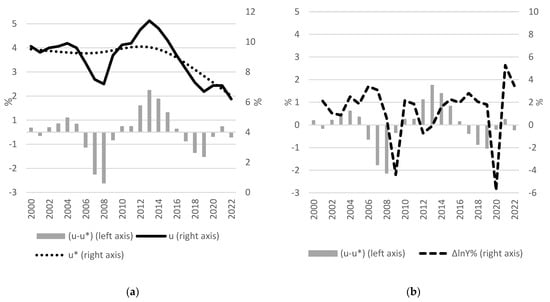
Figure 1.
Total unemployment dynamics for the whole EU-27 panel. (a) Cyclical unemployment or the so-called unemployment gap (u − u*), actual unemployment (u), and estimated equilibrium unemployment (u*). (b) Cyclical unemployment or the so-called unemployment gap (u − u*) and economic growth (ΔlnY%).
For example, in 2009 and 2020, when the negative growth rate was above 4%, the unemployment gap (u − u*) was still slightly negative (the economy was at full employment) since, for several years prior, the economy was constantly expanding, and the actual unemployment rate (u) was low. In contrast, the negative growth rate in 2012 and 2013 was below 1%. Still, the unemployment gap was significantly positive (actual unemployment was above its equilibrium level, i.e., cyclical unemployment) since the economic downturn happened just after the short and not robust recovery period. Considering periods of growth, during 2002–2005, i.e., during the recovery period, there was still a positive unemployment gap which turned negative during 2006–2007 at the later growth stage. In 2008, i.e., over the last year before the crisis hit, the unemployment gap remained significantly negative despite the growth rate being already below 1%. The same is true considering the economic boom period of 2014–2019. Over the first three years of this period, i.e., 2014–2016, when the economy started to recover from the last crisis, the unemployment gap was positive (the economy was not at its full potential and full employment) but steadily decreasing. During 2017–2019, after a longer and more robust period of growth, the unemployment gap turned negative and increased each year. Thus, we see that the size of the gap is a good indicator of whether there is a beginning (positive gap) or an end (negative gap) to the economic growth period. The same is true during an economic downturn, i.e., at its beginning the gap is negative and becomes positive when the crisis becomes long-lasting and severe.
We assume here that growth becomes jobless at the later stages of the growth phase when the economy is working at its full potential, i.e., full employment. To estimate the elasticity, one when the economy is growing and the other when declining over the whole distribution of the unemployment gap, we propose the following specification with three-way interaction:
which, after rearranging, allows estimating conditional elasticities separately for the period of growth and decline over the whole distribution of the unemployment gap:
where the conditional elasticity or conditional slope coefficient of employment growth () on output growth () over the economic boom period (when ) for the whole distribution of the unemployment gap is . Analogously, when the economy is in decline, i.e., when , the slope coefficient has the following expression .
Additionally, our specification includes productivity growth () assuming that the need to employ more people in the short-run positively depends on output growth but negatively on productivity growth, i.e., if productivity grows, the same amount of value added could be created with fewer employed people. We use total factor productivity (TFP) and TFP capital and labor shares as proxies for productivity. Moreover, we augment our specification with ∆lnLMRi,t, i.e., changes in labor market regulation, which we measure by the labor market regulation index of the Fraser Institute. Index values vary from 0 to 10 with higher values meaning a less regulated labor market.
Employment elasticities are estimated for different employment types, i.e., total, male, female employment, and employment by different educational attainment levels of the International Standard Classification of Education (ISCED). ISCED 0–2 corresponds to pre-primary, primary, and lower-secondary education, ISCED levels 3–4—upper-secondary education and post-secondary non-tertiary education, ISCED levels 5–8—tertiary education. Youth corresponds to the group of persons aged 15–24 according to the definition provided by the United Nations.
We do not include factors that might affect the changes in the working-age population, for example, migration, since we use the number of employed people instead of employment level, which might be affected not just by the number of employed people (the numerator) but also the change in the working-age population (the denominator).
Our general estimates are based on OLS since the number of employed people, output, productivity, and labor market regulation enter the equations in their first differences. Thus, unobserved time-fixed country heterogeneity is removed. Since the unemployment gap enters the specification in levels, we re-estimated our specifications with fixed effects (FE) to control the remaining cross-country heterogeneity with a robustness check.
Moreover, the research (Ibragimov and Ibragimov 2017; Huang et al. 2020; Adegboye et al. 2020; Maza 2022; Raies 2023; Christopoulos et al. 2023) emphasizes that the OLS or FE used to estimate the unemployment/employment version of Okun’s equation might produce biased elasticities due to endogeneity caused by the reverse causality running not just from output growth to employment growth but also from employment growth to output growth. Following Adegboye et al. (2020), we used a two-stage least square (TSLS) estimator and one-period lagged total output to output change instrument and addressed the potential endogeneity bias. For an IV to be strong, it should be significantly correlated with a potentially endogenous variable but not with the dependent variable. Based on neoclassical convergence theory, the assumption here is that output growth at the current period is negatively correlated with one-period lagged output. The estimated correlation between output growth and one-period lagged growth was negative and significant (ρ = −0.202, p-value < 0.0001). One-period lagged output was not correlated with total employment change (ρ = −0.060, p-value = 0.1426). Correlations with other types of employment change are presented in Table A1 (see Appendix A). In all cases, correlations are insignificant, thus empirically ensuring the validity of the chosen IV.
We might also consider that employment growth and productivity growth are subject to bidirectional causality and, thus, are another potential source for endogeneity in our specification. We can argue that increasing employment can lead to a larger labor force and potentially higher labor input. It can contribute to economies of scale, specialization, and increased coordination, improving labor productivity. With more workers available, businesses can allocate resources more efficiently and take advantage of the division of labor, leading to higher productivity levels. On the other hand, unplanned increases in employment levels can sometimes lead to reduced labor productivity. If businesses rapidly expand their workforce without adequate training, resources, or infrastructure, this can result in inefficiencies and lower productivity. Insufficient coordination, lack of proper supervision, or skill gaps among new hires can hinder productivity levels. We employed the same strategy as in the case of output change to control the endogeneity of productivity (correlation analysis shows that productivity growth in the current period is negatively correlated with one-period lagged productivity (ρ = −0.369, p-value < 0.0001), and the latter is not correlated with total employment change (ρ = −0.064, p-value = 0.1177)). Correlations between one-period lagged productivity and other types of employment change are presented in Table A1 (see Appendix A). In all cases, correlations are insignificant, thus, empirically ensuring the validity of the chosen IV.
Our estimations are based on EU-27 data covering the period of 2000–2022. All data on the variables are provided by Eurostat, except for the total factor productivity provided by the AMECO database and labor market regulation provided by the Fraser Institute. We opted not to utilize the widely used OECD Employment Protection Legislation indexes as a proxy for labor market regulation in our study due to insufficient data on some EU countries, a shorter time series, and inconsistencies stemming from methodology revisions. The selected period under analysis makes it possible to capture at least two full business cycles. This is important, since our model tests the heterogeneity of elasticities between growth and decline phases and heterogeneity within these phases. Summary statistics of variables are represented in Table 1.

Table 1.
Summary statistics.
The average output growth in the EU during the analyzed period was 2.3%, indicating an overall increase in economic output (see Table 1). However, output changes are accompanied by notable fluctuations, as reflected in a standard deviation of 3.8%. Output fluctuations ranged from the most negative change of −16.1% to the most positive change of 21.8%. In contrast, employment changes showed a different pattern, with an overall average growth of 0.7%, which was more than three times lower than the output growth. The employment landscape exhibited variations based on gender, age groups, and educational attainment levels.
The employment change of the youth and least educated displays a negative average change, suggesting a contraction in employment for these demographic groups. The employment growth of females was higher compared to men and that of the highly educated compared to those with lower education. Such tendencies show the increasing demand for women and highly educated labor, possibly determined by the structural changes in the EU economies.
The average unemployment rate in the EU was 8.4%, with gender, age, and educational disparities apparent. Although the average unemployment rate for females was slightly higher than the total and male unemployment rates, youth and the least educated groups faced significantly higher average unemployment rates and standard deviations. In contrast, highly educated individuals had the lowest average unemployment rate at 4.8%. The same tendencies are revealed in the cases of equilibrium unemployment rates and unemployment gaps in the EU.
On average, total factor productivity changed by 1.1% in the EU. The variations in capital and labor shares suggest that productivity growth was determined more by increased labor productivity than capital productivity. The change in labor market regulation exhibited a mean of 1.4%, indicating a trend towards less rigid labor market regulation in the EU. The standard deviation of 5.7% revealed significant regulatory changes across the observed entities, ranging from significant reductions to substantial increases.
4. Results
After applying the Wooldridge test, we found evidence of minimal negative serial correlation in the first differential errors of pooled OLS estimates. Unlike positive serial correlation, the usual OLS standard errors may not greatly understate the correct standard errors when the errors are negatively correlated. The White test (technically, this test is not valid if there is also serial correlation, but it is strongly suggestive) indicates that errors are heteroscedastic. Finally, the Pesaran CD test shows that the error term is cross-sectionally correlated. To address all these problems, we calculated panel-corrected standard errors (PCSE) for all estimations.
Tests for differing group intercepts suggest that first-differenced variables successfully removed all time-constant country heterogeneity. Thus, compared with pooled OLS, the FE has no noticeable advantage in estimating Equation (3). The Hausman test indicates that the selected instrumental variables are valid. All in all, all estimations yielded very similar coefficients for the equation’s parameters and, thus, further interpretations and discussions will be mainly based on pooled OLS estimates.
Table 2 reports estimates of Equation (3) with the number of total employed people in the economy as the dependent variable. Estimates using specific types of employed persons are presented in Appendix B.
Table 2.
Pooled OLS, FE, and TSLS estimates of Equation (3). Dependent variable—total number of employed people in the economy.
Considering the control variables, the results based on the EU-27 data suggest that if there is no output change, an increase in total factor productivity (TFP) by one percent is associated with a decrease in total employment by 0.62 percent. Breaking down TFP into capital and labor shares, it becomes evident that change in capital productivity has no significant effect, while a positive change in labor productivity has a considerably negative impact on employment opportunities with a fixed amount of output (no output change). Youth employment and the employment of those with the lowest education level (ISCED 0–2) are the categories that reacted to productivity change the most—twice more than total (male and female) and other educational attainment level-specific employment. In line with (Butkus et al. 2023) we find no effect of labor market regulation on employment change.
To visualize the estimation results, i.e., the distribution of all elasticities across the observed range of the unemployment gap, Figure 2 presents the estimated range of point coefficients on elasticities and their 95% confidence interval for the economic growth and decline periods.
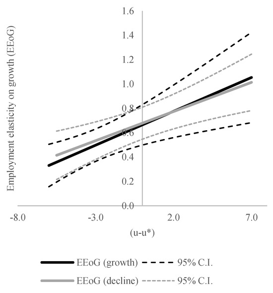
Figure 2.
Conditional (moderated by the unemployment gap) total employment elasticity on growth and its 95% C.I.
Our results strongly suggest that there is no statistically significant difference between elasticities across economic growth and decline periods, i.e., coefficient on the interaction term is insignificant at a 10% level. This conclusion is valid not just in cases when there is no unemployment gap, i.e., , but also for any value of a positive or negative gap since the effect of coefficient on interaction term is also insignificant at a 10% level. This is also evident from Figure 2, since both solid lines (black for the growth period and grey for the decline period) are very close, and their 95% confidence intervals (dashed lines) overlap. We find very similar results for all types of employment. The coefficients of elasticity differ from 0.54 for highly educated people to 1.04 for youth employment, suggesting that youth employment is the most sensitive to output change, followed by the employment of people with the lowest level of education (0.73). The elasticity of female employment (0.63) is slightly smaller than that of males (0.70). Still, they do not statistically significantly differ from the elasticity of total employment (0.66), considering the standard errors of the estimated coefficients.
We found evidence that elasticity was subject to change over the same phase of the business cycle, i.e., over phases of growth and decline. For example, considering total employment, when GDP is growing, and the unemployment gap is positive and high, indicating that the economy is recovering after a severe depression, the estimated coefficient is around unity. Conversely, when the unemployment gap is negative, i.e., the economy is in its late expansion phase, elasticity drops to 0.4, which means that the effect of growth on unemployment change decreases by more than by half. Over the phase of economic decline, we observe very similar tendencies, just in opposite directions. When the economy has just started to decline after a long period of growth (the unemployment gap is negative and GDP is decreasing), the elasticity coefficient is relatively low—around 0.4. Conversely, when GDP is in decline and the unemployment gap is positive, which indicates severe depression, elasticity is high (coefficient is around one), showing an increase by more than two times.
We find very similar results for other types of employment (see Table A2, Table A3, Table A4, Table A5, Table A6 and Table A7 in the Appendix B and Figure 3). The only exceptions are youth and ISCED 0–2 employment, which, according to our estimations, react to GDP change similarly, irrespective of the size of the unemployment gap.
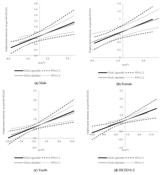
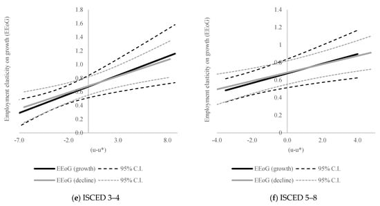
Figure 3.
Conditional (moderated by the unemployment gap) employment elasticity on growth and its 95% C.I. (a) Male employment. (b) Female employment. (c) Youth employment. (d) ISCED 0–2 employment. (e) ISCED 3–4 employment. (f) ISCED 5–8 employment.
The general observed tendency for the EU-27 countries is that elasticity is higher when the unemployment gap is positive and increasing and lower when the gap is negative and decreasing, regardless of the business cycle phase. It suggests that in analyzing the heterogeneity of employment elasticity in terms of growth, we should consider the labor market (unemployment gap) situation more than the direction of GDP change (phase of the business cycle). It can be argued that the ability of growth to increase employment is very limited when the economy operates at its potential level (full employment). Of course, employment can still grow due to labor force immigration or higher participation rates in the labor force, but these factors cannot fully compensate for the bottleneck induced by the lack of unemployed people.
5. Discussion and Conclusions
The research confirms both hypotheses: firstly, that youth and the least educated face the consequences of jobless growth the most (H1); and, secondly, that employment elasticity continuously changes throughout the same phase of the business cycle depending on the maturity of the business cycle phase (H2). The results of the study provide important insights into the analysis of jobless growth, focusing on employment intensity over the business cycle and emphasizing the importance of gender, age, and educational attainment level. We use the unemployment gap as a more precise indicator of business cycle phases, allowing us to analyze not only the elasticity differences between the growth and decline phases but also within these phases. Consistent with Oh (2018) and Donayre (2022), our research results indicate that in previous studies the commonly applied separation of two economic growth regimes (positive and negative output change) is insufficient for understanding the complex relationship between employment and output. The findings suggest that the elasticity of employment is higher when the unemployment gap is positive and increasing, regardless of the business cycle phase. Thus, our results suggest that it is not growth/decline regimes but rather the size of the gap that influences the effect of economic growth on employment. This represents a significant departure from conventional knowledge present in the literature, which traditionally suggests two regime models, i.e., elasticity is subject to change within the same business cycle phase.
The study also reveals that certain groups, such as youth and individuals with the lowest education levels, are more sensitive to the changes in output, which is in line with previous research by (Onaran 2008; Anderson and Braunstein 2013; Butkus et al. 2023). However, the results of this study provide additional insight, indicating that when the economy operates in proximity to its full employment level (i.e., with minimal deviation between actual and natural unemployment levels), the responsiveness of employment for different demographic groups to economic growth or decline tends to approach homogeneity.
The findings of this research have important policy implications for addressing the issue of jobless growth. Policymakers should consider the differences in employment’s reaction to output changes and not the direction of economic growth when designing targeted interventions to address employment. Moreover, disparities in employment can be achieved through targeted interventions such as retraining programs and skill development initiatives to ensure that workers have the necessary skills to meet the demands of evolving industries.
The research has several limitations. Firstly, the analysis of only the EU-27 countries may not reflect global trends. Furthermore, the results may lack generalizability beyond the EU-27 and fail to consider sector-specific trends, potentially limiting their applicability. Additionally, the study’s focus on elasticity within specific business cycle phases might neglect broader economic indicators or external factors influencing employment. Future research should address these limitations by expanding geographical scope, incorporating working-age population dynamics factors, exploring sector-specific impacts, and enabling a more comprehensive understanding of the specific factors that contribute to job growth at different stages of the business cycle, as our results indicate that economic growth is conditioned by an increasing productivity because the reaction of employment is limited.
Author Contributions
Conceptualization, M.B., L.D.-K., K.M., D.R. and J.Š.; methodology, M.B.; formal analysis and investigation, M.B., L.D.-K. and D.R.; resources, K.M. and J.Š.; data curation, L.D.-K. and D.R.; writing—original draft preparation, M.B., L.D.-K., K.M., D.R. and J.Š.; writing—review and editing, M.B., L.D.-K., K.M., D.R. and J.Š. All authors have read and agreed to the published version of the manuscript.
Funding
This research was funded by the Research Council of Lithuania, grant number S-MIP-22-18.
Informed Consent Statement
Not applicable.
Data Availability Statement
The paper uses publicly available data. Sources and data are defined in Section 2.
Conflicts of Interest
The authors declare no conflicts of interest.
Appendix A
Table A1.
Correlation between employment change, output level, and total factor productivity.
Table A1.
Correlation between employment change, output level, and total factor productivity.
| Total | Male | Female | Youth | ISCED 0–2 | ISCED 3–4 | ISCED 5–8 | ||
|---|---|---|---|---|---|---|---|---|
| corr. coef. | −0.0603 | −0.0653 | −0.0519 | 0.0557 | 0.0431 | −0.0580 | −0.0765 | |
| p-value | 0.1426 | 0.1122 | 0.2068 | 0.1755 | 0.2951 | 0.1580 | 0.0626 | |
| corr. coef. | 0.0643 | 0.0426 | 0.0748 | 0.0971 | 0.0748 | −0.0492 | −0.0191 | |
| p-value | 0.1177 | 0.3005 | 0.0689 | 0.0640 | 0.0688 | 0.2312 | 0.6411 | |
Note: Since youth employment correlation with one-period lagged TFP was significant, we used two-period lagged TFP as an instrument. In the case of youth employment, the correlation coefficient is reported with two-period lagged TFP.
Appendix B
Table A2.
Pooled OLS, FE, and TSLS estimates of Equation (3). Dependent variable—number of employed males in the economy.
Table A2.
Pooled OLS, FE, and TSLS estimates of Equation (3). Dependent variable—number of employed males in the economy.
| Pooled OLS | FE | TSLS | ||||
|---|---|---|---|---|---|---|
| const. | α | −0.0020 | −0.0020 | −0.0029 | −0.0018 | |
| (0.0053) | (0.0045) | (0.0054) | (0.0038) | |||
| 0.6987 *** | 0.7062 *** | 0.7098 *** | 0.7277 *** | |||
| (0.0647) | (0.0815) | (0.0848) | (0.1701) | |||
| 0.0423 ** | 0.0440 ** | 0.0357 ** | 0.0401 ** | |||
| (0.0180) | (0.0135) | (0.0179) | (0.0163) | |||
| 0.0304 | 0.0420 | −0.0139 | 0.0426 | |||
| (0.1115) | (0.1226) | (0.1192) | (0.1188) | |||
| 0.0150 | 0.0341 | 0.0197 | 0.0258 | |||
| (0.0245) | (0.0234) | (0.0268) | (0.0246) | |||
| −0.0050 | −0.0037 | −0.0046 | −0.0049 | |||
| (0.0031) | (0.0027) | (0.0030) | (0.0044) | |||
| −0.0029 *** | −0.0017 ** | −0.0026 *** | −0.0034 *** | |||
| (0.0008) | (0.0007) | (0.0007) | (0.0009) | |||
| 0.0021 | 0.0018 ** | 0.0016 | 0.0021 | |||
| (0.0014) | (0.0008) | (0.0015) | (0.0014) | |||
| Total Factor Productivity (TFP) | −0.6082 *** | −0.5647 *** | −0.5549 *** | |||
| (0.0704) | (0.0899) | (0.0773) | ||||
| TFP, Capital share | 0.0024 | |||||
| (0.0534) | ||||||
| TFP, Labor share | −1.2671 *** | |||||
| (0.1819) | ||||||
| 0.0083 | 0.0059 | 0.0049 | 0.0133 | |||
| (0.0136) | (0.0104) | (0.0141) | (0.0138) | |||
| n | 589 | 589 | 589 | 589 | ||
| Adj. R2 | 0.6254 | 0.7021 | 0.6416 | 0.6094 | ||
| p-value for Woldridge 1st order autocorrelation test | 0.0252 | 0.9559 | ||||
| p-value for White’s heteroscedasticity test | 0.0370 | 0.1606 | ||||
| p-value for Pesaran CD test | 0.0030 | 0.0054 | ||||
| p-value of test for differing group intercepts | 0.5046 | |||||
| p-value for Hausman test | 0.2857 | |||||
Note: All estimates include time dummies. Panel-corrected standard errors (PCSE) are presented in parentheses. *, **, and *** indicate significance at the 10, 5, and 1 percent level, respectively.
Table A3.
Pooled OLS, FE, and TSLS estimates of Equation (3). Dependent variable—number of employed females in the economy.
Table A3.
Pooled OLS, FE, and TSLS estimates of Equation (3). Dependent variable—number of employed females in the economy.
| Pooled OLS | FE | TSLS | ||||
|---|---|---|---|---|---|---|
| const. | α | 0.0058 | 0.0057 | 0.0050 | 0.0075 | |
| (0.0043) | (0.0040) | (0.0042) | (0.0089) | |||
| 0.6283 *** | 0.6041 *** | 0.6514 *** | 0.6746 *** | |||
| (0.1442) | (0.1275) | (0.0988) | (0.1300) | |||
| 0.0680 *** | 0.0606 *** | 0.0665 *** | 0.0595 *** | |||
| (0.0244) | (0.0167) | (0.0228) | (0.0203) | |||
| −0.0169 | −0.0263 | −0.0503 | 0.0546 | |||
| (0.1350) | (0.1172) | (0.1269) | (0.3057) | |||
| −0.0249 | −0.0133 | −0.0011 | −0.0068 | |||
| (0.0461) | (0.0334) | (0.0415) | (0.0609) | |||
| −0.0080 *** | −0.0064 ** | −0.0083 *** | −0.0093 *** | |||
| (0.0026) | (0.0025) | (0.0027) | (0.0034) | |||
| −0.0051 *** | −0.0037 *** | −0.0043 *** | −0.0052 *** | |||
| (0.0011) | (0.0009) | (0.0012) | (0.0014) | |||
| 0.0041 *** | 0.0032 | 0.0026 * | 0.0041 *** | |||
| (0.0012) | (0.0012) | (0.0014) | (0.0013) | |||
| Total Factor Productivity (TFP) | −0.6387 *** | −0.6671 *** | −0.6891*** | |||
| (0.1221) | (0.1015) | (0.1229) | ||||
| TFP, Capital share | 0.0024 | |||||
| (0.1134) | ||||||
| TFP, Labor share | −1.3351 *** | |||||
| (0.1823) | ||||||
| 0.0176 | 0.0156 | 0.0193 * | 0.0209 | |||
| (0.0120) | (0.0113) | (0.0108) | (0.0145) | |||
| n | 589 | 589 | 589 | 589 | ||
| Adj. R2 | 0.4434 | 0.5404 | 0.4974 | 0.4370 | ||
| p-value for Woldridge 1st order autocorrelation test | 0.0137 | 0.5889 | ||||
| p-value for White’s heteroscedasticity test | 0.0093 | 0.0002 | ||||
| p-value for Pesaran CD test | 0.0023 | 0.0055 | ||||
| p-value of test for differing group intercepts | 0.3904 | |||||
| p-value for Hausman test | 0.6876 | |||||
Note: All estimates include time dummies. Panel-corrected standard errors (PCSE) are presented in parentheses. *, **, and *** indicate significance at the 10, 5, and 1 percent level, respectively.
Table A4.
Pooled OLS, FE, and TSLS estimates of Equation (3). Dependent variable—number of employed youth in the economy.
Table A4.
Pooled OLS, FE, and TSLS estimates of Equation (3). Dependent variable—number of employed youth in the economy.
| Pooled OLS | FE | TSLS | ||||
|---|---|---|---|---|---|---|
| const. | α | −0.0272 | −0.0250 | −0.0358 * | −0.0067 | |
| (0.0182) | (0.0190) | (0.0184) | (0.0161) | |||
| 1.0435 *** | 1.1463 *** | 1.1061 *** | 1.1960 *** | |||
| (0.2730) | (0.3216) | (0.3109) | (0.4520) | |||
| 0.0147 | 0.0230 | 0.0050 | 0.0346 | |||
| (0.0341) | (0.0325) | (0.0358) | (0.0473) | |||
| 0.3548 | 0.3773 | 0.3625 | 0.3531 | |||
| (0.2640) | 0.2800 | (0.2880) | (0.2719) | |||
| 0.0426 | 0.0541 | 0.0629 | 0.0704 | |||
| (0.0550) | (0.0468) | (0.0555) | (0.0720) | |||
| −0.0122 | −0.0082 | −0.0088 | −0.02734 * | |||
| (0.0103) | (0.0113) | (0.0093) | (0.0143) | |||
| −0.0033 * | −0.0018 | −0.0028 | −0.0039 ** | |||
| (0.0018) | (0.0015) | (0.0018) | (0.0019) | |||
| 0.0009 | −0.0005 | 0.0008 | 0.0004 | |||
| (0.0022) | (0.0019) | (0.0022) | (0.0023) | |||
| Total Factor Productivity (TFP) | −1.1236 *** | −1.1601 *** | −1.1546 *** | |||
| (0.2430) | (0.2995) | (0.2229) | ||||
| TFP, Capital share | 0.3915 | |||||
| (0.3495) | ||||||
| TFP, Labor share | −2.5701 *** | |||||
| (0.4608) | ||||||
| −0.0173 | −0.0210 | −0.0373 | −0.0249 | |||
| (0.0438) | (0.0340) | (0.0413) | (0.0455) | |||
| n | 589 | 589 | 589 | 589 | ||
| Adj. R2 | 0.3814 | 0.4257 | 0.4266 | 0.2839 | ||
| p-value for Woldridge 1st order autocorrelation test | 0.6107 | 0.8784 | ||||
| p-value for White’s heteroscedasticity test | 0.8489 | 0.8956 | ||||
| p-value for Pesaran CD test | 0.0055 | 0.0084 | ||||
| p-value of test for differing group intercepts | 0.5007 | |||||
| p-value for Hausman test | 0.0104 | |||||
Note: All estimates include time dummies. Panel-corrected standard errors (PCSE) are presented in parentheses. *, **, and *** indicate significance at the 10, 5, and 1 percent level, respectively.
Table A5.
Pooled OLS, FE, and TSLS estimates of Equation (3). Dependent variable—number of employed people with ISCED 0–2 education in the economy.
Table A5.
Pooled OLS, FE, and TSLS estimates of Equation (3). Dependent variable—number of employed people with ISCED 0–2 education in the economy.
| Pooled OLS | FE | TSLS | ||||
|---|---|---|---|---|---|---|
| const. | α | −0.0097 | −0.0092 | −0.0167 | 0.0015 | |
| (0.0183) | (0.0190) | (0.0188) | (0.0189) | |||
| 0.7251 *** | 0.7379 ** | 0.7251 *** | 0.7200 *** | |||
| (0.2427) | (0.2803) | (0.2095) | (0.2419) | |||
| 0.0569 | 0.0239 | 0.0577 | 0.0388 | |||
| (0.0344) | (0.0409) | (0.0341) | (0.0436) | |||
| 0.3178 | 0.3144 | 0.0200 | 0.7096 | |||
| (0.2627) | (0.2701) | (0.2369) | (0.4832) | |||
| 0.0049 | 0.0281 | 0.0351 | 0.0435 | |||
| (0.0552) | (0.0600) | (0.0509) | (0.0809) | |||
| −0.0130 | −0.0105 | −0.0120 | −0.0231 | |||
| (0.0104) | (0.0101) | (0.0106) | (0.0143) | |||
| 0.0062 *** | −0.0051 *** | −0.0059 *** | −0.0063 *** | |||
| (0.0016) | (0.0016) | (0.0018) | (0.0015) | |||
| 0.0032 | 0.0025 | 0.0044 | 0.0031 | |||
| (0.0028) | (0.0028) | (0.0030) | (0.0026) | |||
| Total Factor Productivity (TFP) | −1.0102 *** | −1.0112 *** | −0.4571 | |||
| (0.2120) | (0.2080) | (0.8440) | ||||
| TFP, Capital share | 0.1028 | |||||
| (0.4567) | ||||||
| TFP, Labor share | −1.9146 *** | |||||
| 0.3103 | ||||||
| 0.0323 | 0.0330 | 0.0164 | 0.0505 | |||
| (0.0490) | (0.0448) | (0.0401) | (0.0508) | |||
| n | 589 | 589 | 589 | 589 | ||
| Adj. R2 | 0.2333 | 0.2505 | 0.2829 | 0.2139 | ||
| p-value for Woldridge 1st order autocorrelation test | 0.6177 | 0.5790 | ||||
| p-value for White’s heteroscedasticity test | 0.0062 | 0.0157 | ||||
| p-value for Pesaran CD test | 0.0288 | 0.0221 | ||||
| p-value of test for differing group intercepts | 0.2700 | |||||
| p-value for Hausman test | 0.3643 | |||||
Note: All estimates include time dummies. Panel-corrected standard errors (PCSE) are presented in parentheses. *, **, and *** indicate significance at the 10, 5, and 1 percent level, respectively.
Table A6.
Pooled OLS, FE, and TSLS estimates of Equation (3). Dependent variable—number of employed people with ISCED 3–4 education in the economy.
Table A6.
Pooled OLS, FE, and TSLS estimates of Equation (3). Dependent variable—number of employed people with ISCED 3–4 education in the economy.
| Pooled OLS | FE | TSLS | ||||
|---|---|---|---|---|---|---|
| const. | α | 0.0081 | 0.0100 | 0.0072 | 0.0051 | |
| (0.0180) | (0.0194) | (0.0171) | (0.0254) | |||
| 0.6153 *** | 0.6305 *** | 0.6091 *** | 0.5779 *** | |||
| (0.2094) | (0.2148) | (0.1327) | (0.1444) | |||
| 0.1020 ** | 0.0686 ** | 0.0700 * | 0.1097 ** | |||
| (0.0420) | (0.0346) | (0.0398) | (0.0477) | |||
| −0.0041 | −0.0082 | 0.0505 | −0.0906 | |||
| (0.1783) | (0.1583) | (0.1604) | (0.4973) | |||
| −0.0273 | −0.0125 | −0.0281 | −0.0254 | |||
| (0.0513) | (0.0511) | (0.0494) | (0.0806) | |||
| −0.0070 | −0.0055 | −0.0100 | −0.0047 | |||
| (0.0084) | (0.0084) | (0.0093) | (0.0079) | |||
| −0.0058 *** | −0.0048 *** | −0.0039 ** | −0.0063 *** | |||
| (0.0017) | (0.0017) | (0.0015) | (0.0022) | |||
| 0.0055 ** | 0.0046 * | 0.0019 | 0.0058 ** | |||
| (0.0023) | (0.0023) | (0.0020) | (0.0026) | |||
| Total Factor Productivity (TFP) | −0.4833 *** | −0.4786 *** | −0.4855 *** | |||
| (0.1980) | (0.1868) | (0.1562) | ||||
| TFP, Capital share | 0.2362 | |||||
| (0.2468) | ||||||
| TFP, Labor share | −1.0986 *** | |||||
| (0.2599) | ||||||
| 0.0366 | 0.0348 | 0.0316 | 0.0388 | |||
| (0.0250) | (0.0266) | (0.0279) | (0.0258) | |||
| n | 589 | 589 | 589 | 589 | ||
| Adj. R2 | 0.2176 | 0.2457 | 0.2889 | 0.2109 | ||
| p-value for Woldridge 1st order autocorrelation test | 0.0050 | 0.0172 | ||||
| p-value for White’s heteroscedasticity test | 0.0021 | 0.0020 | ||||
| p-value for Pesaran CD test | 0.0129 | 0.0311 | ||||
| p-value of test for differing group intercepts | 0.3806 | |||||
| p-value for Hausman test | 0.6243 | |||||
Note: All estimates include time dummies. Panel-corrected standard errors (PCSE) are presented in parentheses. *, **, and *** indicate significance at the 10, 5, and 1 percent level, respectively.
Table A7.
Pooled OLS, FE, and TSLS estimates of Equation (3). Dependent variable—number of employed people with ISCED 5–8 education in the economy.
Table A7.
Pooled OLS, FE, and TSLS estimates of Equation (3). Dependent variable—number of employed people with ISCED 5–8 education in the economy.
| Pooled OLS | FE | TSLS | ||||
|---|---|---|---|---|---|---|
| const. | α | −0.0019 | −0.0027 | 0.0001 | −0.0034 | |
| (0.0240) | (0.0237) | (0.0240) | (0.0206) | |||
| 0.5396 *** | 0.5358 *** | 0.5401 *** | 0.4979 *** | |||
| (0.1784) | (0.1830) | (0.1440) | (0.2025) | |||
| 0.0695 ** | 0.0642 * | 0.0734 ** | 0.0650 * | |||
| (0.0325) | (0.0360) | (0.0351) | (0.0391) | |||
| −0.0322 | 0.0029 | −0.0237 | −0.0638 | |||
| (0.1741) | (0.1645) | (0.1364) | (0.4248) | |||
| 0.1196 | 0.1401 | 0.1618 * | 0.1129 | |||
| (0.0962) | (0.0988) | (0.0889) | (0.1429) | |||
| −0.0049 | −0.0035 | −0.0031 | −0.0035 | |||
| (0.0058) | (0.0055) | (0.0056) | (0.0102) | |||
| −0.0004 | 0.0017 | 0.0011 | −0.0011 | |||
| (0.0036) | (0.0037) | (0.0039) | (0.0050) | |||
| 0.0048 | 0.0040 | 0.0018 | 0.0050 | |||
| (0.0043) | (0.0040) | (0.0050) | (0.0046) | |||
| Total Factor Productivity (TFP) | −0.5827 ** | −0.5917 ** | −0.5511 *** | |||
| (0.2340) | (0.2430) | (0.1879) | ||||
| TFP, Capital share | −0.2269 | |||||
| (0.2170) | ||||||
| TFP, Labor share | −1.1254 ** | |||||
| (0.4646) | ||||||
| 0.0009 | −0.0016 | 0.0113 | 0.0030 | |||
| (0.0585) | (0.0592) | (0.0555) | (0.0599) | |||
| n | 585 | 585 | 585 | 585 | ||
| Adj. R2 | 0.0543 | 0.0663 | 0.1004 | 0.0528 | ||
| p-value for Woldridge 1st order autocorrelation test | 0.9624 | 0.9500 | ||||
| p-value for White’s heteroscedasticity test | 0.4185 | 0.4786 | ||||
| p-value for Pesaran CD test | 0.8920 | 0.8860 | ||||
| p-value of test for differing group intercepts | 0.5429 | |||||
| p-value for Hausman test | 0.9256 | |||||
Note: All estimates include time dummies. Panel-corrected standard errors (PCSE) are presented in parentheses. *, **, and *** indicate significance at the 10, 5, and 1 percent level, respectively.
References
- Adegboye, Abidemi, Monday Egharevba, and Joel Edafe. 2019. Economic Regulation and Employment Intensity of Output Growth in Sub-Saharan Africa. In Governance for Structural Transformation in Africa. Berlin and Heidelberg: Springer, pp. 101–43. [Google Scholar] [CrossRef]
- Adegboye, Abidemi, Monday Nwaogu, and Monday Egharevba. 2020. Economic Policies and Employment Elasticity of Growth in Sub-Saharan Africa. The Nigerian Journal of Economic and Social Studies 62: 335–67. [Google Scholar]
- Aguiar-Conraria, Luís, Manuel M. F. Martins, and Maria Joana Soares. 2020. Okun’s Law across Time and Frequencies. Journal of Economic Dynamics and Control 116: 103897. [Google Scholar] [CrossRef]
- Ajilore, Taiwo, and Olalekan Yinusa. 2011. An analysis of employment intensity of sectoral output growth in Botswana. Southern African Business Review 15: 1–17. [Google Scholar]
- An, Zidong, John Bluedorn, and Gabriele Ciminelli. 2022. Okun’s Law, Development, and Demographics: Differences in the Cyclical Sensitivities of Unemployment across Economy and Worker Groups. Applied Economics 54: 4227–39. [Google Scholar] [CrossRef]
- Anderson, Bret, and Elissa Braunstein. 2013. Economic Growth and Employment from 1990–2010: Explaining Elasticities by Gender. Review of Radical Political Economics 45: 269–77. [Google Scholar] [CrossRef]
- Ben Salha, Ousama, and Mourad Zmami. 2021. The Effect of Economic Growth on Employment in GCC Countries. Scientific Annals of Economics and Business 68: 25–41. [Google Scholar] [CrossRef]
- Berger, David. 2012. Countercyclical Restructuring and Jobless Recoveries. Paper presented at Society for Economic Dynamics 2012 Meeting, Madison, WI, USA, June 28–30; p. 1179. [Google Scholar]
- Burger, John D., and Jeremy S. Schwartz. 2018. Jobless Recoveries: Stagnation or Structural Change? Economic Inquiry 56: 709–23. [Google Scholar] [CrossRef]
- Burggraeve, Koen, Grégory de Walque, and Helene Zimmer. 2015. The relationship between economic growth and employment. Economic Review 1: 32–52. [Google Scholar]
- Butkus, Mindaugas, and Janina Seputiene. 2019. The Output Gap and Youth Unemployment: An Analysis Based on Okun’s Law. Economies 7: 108. [Google Scholar] [CrossRef]
- Butkus, Mindaugas, Laura Dargenytė-Kacilevičienė, Kristina Matuzevičiūtė, Dovilė Ruplienė, and Janina Šeputienė. 2022. Do Gender and Age Matter in Employment—Sectoral Growth Relationship Over the Recession and Expansion. Ekonomika 101: 38–51. [Google Scholar] [CrossRef]
- Butkus, Mindaugas, Laura Dargenytė-Kacilevičienė, Kristina Matuzevičiūtė, Janina Šeputienė, and Dovilė Ruplienė. 2023. Age- and Gender-Specific Output-Employment Relationship across Economic Sectors. Ekonomický Časopis 71: 3–22. [Google Scholar] [CrossRef]
- Christopoulos, Dimitris, Peter McAdam, and Elias Tzavalis. 2023. Exploring Okun’s Law Asymmetry: An Endogenous Threshold Logistic Smooth Transition Regression Approach. Oxford Bulletin of Economics and Statistics 85: 123–58. [Google Scholar] [CrossRef]
- Crivelli, Ernesto, Davide Furceri, and Joël Toujas-Bernaté. 2012. Can Policies Affect Employment Intensity of Growth? A Cross-Country Analysis. Washington: International Monetary Fund, p. 33. [Google Scholar]
- Dahal, Madhav Prasad, and Hemant Rai. 2019. Employment Intensity of Economic Growth: Evidence from Nepal. Economic Journal of Development Issues 27: 34–47. [Google Scholar] [CrossRef]
- Donayre, Luiggi. 2022. On the Behavior of Okun’s Law across Business Cycles. Economic Modelling 112: 105858. [Google Scholar] [CrossRef]
- Duran, Hasan. 2022. Validity of Okun’s Law in a Spatially Dependent and Cyclical Asymmetric Context. Panoeconomicus 69: 447–80. [Google Scholar] [CrossRef]
- Eichengreen, Barry, and Poonam Gupta. 2011. The Service Sector as India’s Road to Economic Growth. Cambridge: National Bureau of Economic Research, p. w16757. [Google Scholar] [CrossRef]
- El-Hamadi, Youssef, Abdeljabbar Abdouni, and Karima Bouaouz. 2017. The sectoral employment intensity of growth in Morocco: A pooled mean group approach. Applied Econometrics and International Development 17: 87–98. [Google Scholar]
- Elroukh, Ahmed W., Alex Nikolsko-Rzhevskyy, and Irina Panovska. 2020. A Look at Jobless Recoveries in G7 Countries. Journal of Macroeconomics 64: 103206. [Google Scholar] [CrossRef]
- Farole, Thomas, Esteban Ferro, and Veronica Michel Gutierrez. 2017. Job Creation in the Private Sector: An Exploratory Assessment of Patterns and Determinants at the Macro, Sector, and Firm Levels. Washington: World Bank. [Google Scholar]
- Furceri, Davide, João Tovar Jalles, and Prakash Loungani. 2020. On the Determinants of the Okun’s Law: New Evidence from Time-Varying Estimates. Comparative Economic Studies 62: 661–700. [Google Scholar] [CrossRef]
- Haider, Azad, Sunila Jabeen, Wimal Rankaduwa, and Farzana Shaheen. 2023. The Nexus between Employment and Economic Growth: A Cross-Country Analysis. Sustainability 15: 11955. [Google Scholar] [CrossRef]
- Huang, Gang, Ho-Chuan Huang, Xiaojian Liu, and Jiangang Zhang. 2020. Endogeneity in Okun’s Law. Applied Economics Letters 27: 910–14. [Google Scholar] [CrossRef]
- Ibragimov, Marat, and Rustam Ibragimov. 2017. Unemployment and Output Dynamics in CIS Countries: Okun’s Law Revisited. Applied Economics 49: 3453–79. [Google Scholar] [CrossRef]
- ILO. 2014. Global Employment Trends 2014—Risk of a Jobless Recovery? Geneva: ILO. [Google Scholar]
- Jha, Srirang, and Amiya Kumar Mohapatra. 2020. Jobless Growth in India: The Way Forward. Journal of Politics & Governance 8: 25–31. [Google Scholar]
- Kapsos, Steven. 2006. The Employment Intensity of Growth: Trends and Macroeconomic Determinants. In Labor Markets in Asia. Edited by Jesus Felipe and Rana Hasan. London: Palgrave Macmillan, pp. 143–201. [Google Scholar] [CrossRef]
- Kim, Jun, Jong Cheol Yoon, and Sang Young Jei. 2020. An Empirical Analysis of Okun’s Laws in ASEAN Using Time-Varying Parameter Model. Physica A: Statistical Mechanics and Its Applications 540: 123068. [Google Scholar] [CrossRef]
- Klinger, Sabine, and Enzo Weber. 2020. GDP-Employment Decoupling in Germany. Structural Change and Economic Dynamics 52: 82–98. [Google Scholar] [CrossRef]
- Lavopa, Alejandro, and Adam Szirmai. 2012. Industrialization, Employment and Poverty. In UNU-MERIT Working Paper Series 2012. #2012-081. Maastricht: Maastricht Economic and Social Research and Training Centre on Innovation and Technology. Available online: https://www.merit.unu.edu/publications/wppdf/2012/wp2012-081.pdf (accessed on 15 March 2023).
- Martus, Bettina Szandra. 2016. Jobless growth: The impact of structural changes. Public Finance Quarterly 61: 244. [Google Scholar]
- Maza, Adolfo. 2022. Regional Differences in Okun’s Law and Explanatory Factors: Some Insights From Europe. International Regional Science Review 45: 555–80. [Google Scholar] [CrossRef]
- Mihajlović, Vladimir, and Gordana Marjanović. 2021. Challenges of the Output-Employment Growth Imbalance in Transition Economies. Naše Gospodarstvo/Our Economy 67: 1–9. [Google Scholar] [CrossRef]
- Mkhize, Njabulo Innocent. 2019. The sectoral employment intensity of growth in South Africa. Southern African Business Review 23: 1–24. [Google Scholar] [CrossRef]
- Novák, Marcel, and Ľubomír Darmo. 2019. Okun’s Law over the Business Cycle: Does It Change in the EU Countries after the Financial Crisis? Prague Economic Papers 28: 235–54. [Google Scholar] [CrossRef]
- Oh, Jong-seok. 2018. Changes in Cyclical Patterns of the USA Labor Market: From the Perspective of Nonlinear Okun’s Law. International Review of Applied Economics 32: 237–58. [Google Scholar] [CrossRef]
- Onaran, Ozlem. 2008. Jobless Growth in the Central and East European Countries: A Country-Specific Panel Data Analysis of the Manufacturing Industry. Eastern European Economics 46: 90–115. [Google Scholar] [CrossRef]
- Pattanaik, Falguni, and Narayan Chandra Nayak. 2014. Macroeconomic determinants of employment intensity of growth in India. The Journal of Applied Economic Research 8: 137–54. [Google Scholar] [CrossRef]
- Porras-Arena, M. Sylvina, and Ángel L. Martín-Román. 2023. The Heterogeneity of Okun’s Law: A Metaregression Analysis. Economic Modelling 128: 106490. [Google Scholar] [CrossRef]
- Raies, Asma. 2023. Sustainable Employment in Developing and Emerging Countries: Testing Augmented Okun’s Law in Light of Institutional Quality. Sustainability 15: 3088. [Google Scholar] [CrossRef]
- Tang, Bo, and Carlos Bethencourt. 2017. Asymmetric Unemployment-Output Tradeoff in the Eurozone. Journal of Policy Modeling 39: 461–81. [Google Scholar] [CrossRef]
- Varghese, N. V., and Mona Khare. 2021. Employment and Employability of Higher-Education Graduates: An Overview. In India Higher Education Report. Delhi: Routledge, pp. 1–21. [Google Scholar]
- Wang, Xiuhua, and Ho-Chuan Huang. 2017. Okun’s Law Revisited: A Threshold in Regression Quantiles Approach. Applied Economics Letters 24: 1533–41. [Google Scholar] [CrossRef]
- Wolnicki, Miron, Eugeniusz Kwiatkowski, and Ryszard Piasecki. 2006. Jobless Growth: A New Challenge for the Transition Economy of Poland. International Journal of Social Economics 33: 192–206. [Google Scholar] [CrossRef]
Disclaimer/Publisher’s Note: The statements, opinions and data contained in all publications are solely those of the individual author(s) and contributor(s) and not of MDPI and/or the editor(s). MDPI and/or the editor(s) disclaim responsibility for any injury to people or property resulting from any ideas, methods, instructions or products referred to in the content. |
© 2024 by the authors. Licensee MDPI, Basel, Switzerland. This article is an open access article distributed under the terms and conditions of the Creative Commons Attribution (CC BY) license (https://creativecommons.org/licenses/by/4.0/).