Abstract
The existence of fluctuations is part of the narrative, especially when there is a slowdown (or worse, a contraction) in economic activity. The presence of long waves with a period of about 50 years as proposed by Kondratieff is one of the most controversial and fascinating theories about economic cycles. This paper analyses both the original Kondratieff data (from which the hypothesis started) and a dataset that includes GDP per capita for several significant countries. By applying the wavelet analysis (WA), the main objective of the paper is to understand whether it is plausible to support the existence of periodic fluctuations consistent with long cycles theory. The outcomes for Kondratieff’s original dataset do not show the presence of a coherent periodicity for most cases. The same conclusion can be drawn for all the GDP per capita series.
JEL Classifications:
C22; E32; E37; O40
1. Introduction
The plausibility of the existence of recurring phases of growth and decline of the economy seems to be suggested by the oscillations experienced over time. Taking the 2007–2008 global financial crisis as an example, boom–bust changes in financial variables were key determinants in understanding fluctuations in economic activity (Cheng and Chen 2021; Petrakos et al. 2023). The COVID pandemic (Svabova et al. 2022) and the Russia–Ukraine conflict are other recent examples of tensions giving rise to serious concerns. The prevention of dangers and shocks for the entire economic system has become the main objective of macro-prudential policies (Belkhir et al. 2022). The potential existence of regular empirical periodicity within economic systems gained its own merit when the strand of research promoting the theory of the existence of a general business cycle emerged (Aftalion 1909; Pigou 1927; Frisch 1933). This idea is implicit in classical economics and is called the ergodic axiom (Davidson 2015). According to this hypothesis, all economic agents “know the future” through the information from the past and are guided by “rational expectations”. Originally introduced by Muth (1960, 1961), the concept of rational expectations was developed about a decade later for stabilization policy issues by Lucas (1972, 1973), and then for the establishment of “an apparent equilibrium theory of the business cycle” (Lucas 1977) as reported by Kantor (1979). Now, the theoretical basis for considering business cycle volatility as a normal part of a growing economy rests on the real business cycle approach (Almeshari et al. 2023). This idea stems from the seminal and inspiring contribution of Nelson and Plosser (1982) who distinguished between stationary oscillations of output around a deterministic trend and non-stationarity resulting from accumulation over time. Real business cycle theory considers that fluctuations in output are attributable to real shocks which, by influencing the economy, cause it to subsequently adjust toward equilibrium (Gali 1999; Aiyagari 1994; Watson 1993). Similar but not identical are the neo-Keynesian models which, while sharing some basic aspects (such as the rationality of expectations), do not assume a rapid adjustment of the market through an immediate response of prices to changes in the money stock (Silvestre 1993; Gordon 1990). A financial and self-reinforcing origin of economic shocks is explained by Minsky (1992) in his financial instability hypothesis.
The literature on economic cycles attempts a very specific classification based on their average duration (Reijnders 2009): the Kitchin cycles (3–5 years), the Juglar cycles (7–12 years), the Kuznets cycles (15–25 years), the Kondratieff cycles (40–60 years) and, finally, the hegemonial cycles (over 60 years). Within this classification, Kondratieff’s theory of long waves (K-waves) deserves special mention, due to the academic disputes it has generated over the decades. In short, the long-wave theory holds that economic systems are characterized by fluctuation of about 50 years. Probably the first studies on the existence of oscillations within the economy were conducted in the early 20th century through a pioneering contribution by Tugan-Baranowsky (1901). However, as Reijnders (1988) pointed out, van Gelderen (1913)—publishing under the pseudonym of J. Fedder—De Wolf (1924, 1929) and above all Kondratieff (1926, with an English widespread translated version in Kondratieff 1935) followed by Schumpeter (1939) were the most famous authors in this field (Growiec et al. 2018). Undoubtedly, in this specific context, the long waves (or Kondratieff’s waves, K-waves) are probably the ones that have ignited the most relevant debate by meeting the greatest opposition (Devezas and Corredine 2001; Hilmola 2007).
Taking the degree of controversy as the driving factor, the first aim of this paper is to apply a wavelet analysis (WA) to explore the original data presented in Kondratieff’s (1926) article. This fills an existing gap in the literature by overcoming the limitations encountered in processing the original Kondratieff dataset by harmonic analysis (HA). This first point allows us to corroborate (or not) the existence of these long periodic cycles precisely from the data that inspired their theorization.
Another purpose of the present work is to analyze longer and current time series to investigate the potential presence of long waves in the economy. Any confirmation of a cyclical fluctuation can be useful in order to analyze the current economic trend as well. To this aim, we use real Gross Domestic Product (GDP) per capita data from different countries. Despite criticism, GDP remains the leading indicator used internationally to represent (macro)economic performance. Recent contributions with the same goal (but focusing on the movements of profitability) are those proposed by Tsoulfidis and Papageorgiou (2019) and Tsoulfidis and Tsaliki (2022).
The application of WA to both datasets does not allow us to support the theory. The only exceptions we found are related to the Kondratieff price series. Without any claim to be a policy analysis paper, this work contributes to the strand of the literature investigating the deterministic or stochastic nature of macroeconomic fluctuations. Our efforts are in the direction of investigating the plausibility of this controversial theory with the most appropriate data and analysis technique.
2. Data and Methodology
The initial methods for exploring long waves in economic time series were based on the decomposition approach. In this classical procedure, it is assumed that the observed time series is a sum of four different unobserved components: trend, cyclicality, seasonality and irregularity (or noise). Through the combination of smoothing and detrending techniques, it is possible to isolate the major fluctuations of a variable around its trend. Among the assumptions adopted for estimation, the essential pre-requisite for the calculation, there is the definition of a particular form (linear, quadratic, exponential, etc.). Kondratieff’s original analysis based on a moving-average indicator was criticized considering the Slutsky (1927) and Yule (1927) effect induced on cycle-free data (Garvy 1943). Since the 1980s, more refined statistical and mathematical tools have been applied to analyze economic variables and detect the presence of periodical swings. On this point, it is possible to list correlation analysis (Goldstein 1988), filter design (Metz 1992; Metz and Stier 1992), fractional integrated long memory processes (Diebolt 2005), log-linear trends (Bieshaar and Kleinknecht 1984), outlier identification and trend breaks in stochastic models (Darné and Diebolt 2004; Metz 2011), polynomial regression by the best fitting function (Taylor 1988), spectral analysis (van Ewijk 1982; Haustein and Neuwirth 1982; Rasmussen et al. 1989; Reijnders 1990; Gerster 1992; Metz 1992, 2006; Berry 2006; Diebolt and Doliger 2006; Korotayev and Tsirel 2010; Focacci 2017), and structural time series models (Goldstein 1999). Within this general framework, spectral methods and filter design have exerted a paramount role.
Since we are interested in assessing the plausibility of the existence of a periodicity of about 50 years in the economy (Kondratieff’s hypothesis), we built two different datasets.
The first one includes all the original data presented by Kondratieff (1926) as they can be retrieved in Gattei (1981):
- -
- England—Index number of commodity prices 1780–1922 (to simplify correct identification, we marked them with a capital letter, and begin with A);
- -
- France—Index number of commodity prices 1858–1922 (B);
- -
- USA—Index number of commodity prices 1791–1922 (C);
- -
- England—Quotations of interest-bearing securities 1816–1922 (D);
- -
- France—Quotations of interest-bearing securities 1814–1922 (E);
- -
- England—Index of Weekly wages in agriculture 1789–1913 (F) and Cotton Textiles 1807–1913 (G);
- -
- France—Foreign trade 1827–1913 in per capita francs (H);
- -
- England—Coal production 1855–1917 in t/1000 inhabitant (I);
- -
- France—Coal consumption 1827–1913 in t/1000 inhabitant (J);
- -
- England—Pig iron production 1840–1914 in t/1000 inhabitant (K);
- -
- England—Lead production 1855–1920 in t/1000 inhabitant (L).
We chose these data because they are the ones from which all the literature related to the theory of the existence of long cycles originates. As can be seen, the Kondratieff dataset does not only include price series. This aspect is relevant and will be taken up in the next section. Also relevant is the fact that, in Kondratieff’s time, the wavelet technique did not exist. Such a methodology has never been applied to these specific series. The original data of Kondratieff was analyzed through a Fourier transform with spectral analysis for the first time by Focacci (2017). Metz (2011) analyzed only one among the time series proposed by Kodratieff by adopting spectral methods, while van Ewijk (1982) focused his research on outliers identification, modelling and bandwidth of filtering process. In these specific series the spectral detection and the existence of waves is generally disputed because the samples contain too few observations for rigorous testing. Sample size is a crucial issue for periodicity detections through spectral analysis (Adelman 1965; Harkness 1968; Berry 2000). On this aspect, the literature proposes different suggestions: for Klotz and Neal (1973), there is the need of a repetition of at least three (hypothesized) sequences (in this case thus a sample length in the range of 150 ≤ N ≤ 195); Granger and Hatanaka (1964) suggest the repetition of seven cycles (350 ≤ N ≤ 455), while Soper (1975) recommends a minimum of ten repetitions (500 ≤ N ≤ 650).
The second dataset is built from the Maddison Project Database (MPD 2020). It includes yearly series of Gross Domestic Product per capita in 2011 USD for several major countries. Specific sources are detailed and listed following the website’s citation policy. Despite adverse theoretical criticisms and opinions that question its real effectiveness in representing people’s overall well-being, GDP per capita remains the most widely used indicator for measuring economic growth. The GDP growth rate is not re-proposed here. In fact, this indicator, combining different data sources, has already been investigated with spectral methods by Korotayev and Tsirel (2010). However, both the combination of different sources (perhaps also to be evaluated in terms of homogeneity) and the choice to focus on the GDP growth rate make their approach completely different from the one adopted in this work. In brackets, the time span jointly with the integrative data source as advised in MPD for the following:
- -
- Brazil (1850–2018; Barro and Ursua 2008);
- -
- France (1280–2018; Ridolfi 2016);
- -
- Germany (1850–2018);
- -
- India (1884–2018);
- -
- Italy (1310–2018; Baffigi 2011; Malanima 2010);
- -
- Japan (1885–2018; Fukao et al. 2015);
- -
- Turkey (1913–2018);
- -
- UK (1252–2018; Broadberry et al. 2015);
- -
- USA (1800–2018; Sutch 2006);
- -
- Former USSR (1885–2018; Gregory 1982 and Markevich and Harrison 2011).
At the moment, 2018 is the last observation included within MPD.
Precisely to take into account the perplexities of the sceptics who criticize the sample length for invalidating the robustness of the investigation, it was decided to use the longest available series of per capita GDP taken from the most common source cited in the macroeconomic literature. It is important to point out that the original series retrievable from the MPD are in many cases longer. This is the case of Brazil, for example, which, however, presents a considerable degree of temporal discontinuity. For this reason, we select each sample starting from the first year in which the data flow has no interruptions.
Regarding the methodology, we can underline that the WA is a powerful mathematical tool for the analysis of time series in the time-frequency domain able to overcome main drawbacks of HA (Kaiser 2011). Substantially, the HA—also known as Fourier Analysis (FA)—is a filtering approach. It decomposes a series y(t) into a sum of sinusoidal components with different frequencies (Bloomfield 2000). The Discrete Fourier Transform (DFT) is adopted to convert the time domain of a series y(t) into its corresponding frequency domain components following
for n = 0, 1, 2, …, wherein: −Zn = the complex number resulting from the DFT formed by a real (a) and an imaginary part identified by a lower-case i (ib);
- -
- T = the last term of the discrete series;
- -
- e = Euler’s number (also known as Nepier’s constant equal to 2.71…);
- -
- i = is the conventional for imaginary part;
- -
- = is the radians representation of the frequency (fnt).
To speed up iteration in processing, the class of algorithms called fast Fourier transform (FFT) is usually employed to perform a ‘spectral analysis aimed at identifying significant cyclical periods by calculating the power spectrum’ (Warner 1998). The Periodogram Intensities (Ik) can be mathematically derived as
where:
ak and bk are the coefficients of the numbers Zn for k = 1, 2, …, K (K the last time period until the Nyquist–Shannon frequency, i.e., the minimum sampling period needed in order to identify a possible periodicity, usually represented as: 0 ≤ f ≤ 0.5 f).
The sum of Periodogram Intensities represents all the variance of the time series (Box et al. 2016):
Nevertheless, this approach has two inherent disadvantages: a stationary behavior and the absence of a correct positioning of the cyclic components over time. For these reasons, data are usually pre-treated with proper detrending procedures (first differencing for example). Similar considerations apply to bandpass filtering applications such as the common time domain filters of Baxter and King (1999) and/or Christiano and Fitzgerald (2003). For what concerns the correct positioning of the periodic component, in FA methods, a single disturbance affects all frequencies along the entire dataset through the sum of sine and cosine functions. For the Heisemberg uncertainty principle, the higher the certainty about the measurement of one dimension (e.g., frequency), the less certainty it can be related to the other dimension (e.g., time location in time series analysis). The WA methodology succeeds in solving all the previous problems. Unlike the FA, however, its transform is localized both in time and in its functional components (Rhif et al. 2019). This property makes it particularly suitable for the treatment of series with unit roots (Torrence and Compo 1998; Aristizabal and Glavinovic 2003; Cazelles et al. 2008; Sleziak et al. 2015). For this reason, the investigation of a mean reverting behavior is unnecessary (and. therefore, not included here). Furthermore, as pointed out by Beaudry et al. (2020), the elimination of trend can create spurious cycles. The approximations generated by the procedure are robust-to-small variations (Gallegati et al. 2017). The WA provides an efficient way to deal with variables lasting for a finite time, or showing markedly different behavior in their time sequence (Daubechies 1990; Crowley 2007). In fact, unlike spectral methods, wavelets can detect irregularly spaced cyclic components. Considering that WA is very suitable for investigating nonlinear time series, we propose to explore our data also through two specific tests: the Keenan test (Keenan 1985) and the Brock–Dechert–Scheinkman (Brock et al. 1996) BDS test.
A key advantage of WA over Fourier methods (or even spline regression models) lies in the ability to handle with randomly occurring shocks by distorting a dynamical system in which statistical properties change across periods. Ramsey and Lampard (1998a, 1998b) made pioneering contributions using the WA for the investigation of economic relationships. The comparison with the (Self Exciting) Threshold AutoRegressive models (TAR and SETAR), originally introduced by Tong (1978), highlights the good local properties of the WA in catching jumps and transient phenomena, tackling the limits these models encounter in the definition both of the number and the threshold estimation (Li and Xie 1999). Without entering into excessive mathematical details retrievable in specific references also for economic and finance applications (see for example Percival and Walden 2000; Gençay et al. 2001; Ramsey 2002; Schleicher 2002; Gallegati and Semmler 2014), wavelets are small waves (or wave packets) representing the varying duration of the components of a time series (Walker 2008). The wavelet transform (WT) is an integral transformation, which allows for obtaining time–frequency information about data. There are several types of wavelet functions with their own characteristics. The Daubechies, Haar, Mexican Hat and Morlet are among the most widespread. In general, we can identify a “father” (ϕ) and a “mother” (φ) wavelet. The first integrates to 1 and the second to 0:
and
In essence, the “father” (or scaling function S) represents the low-frequency part of the series in the transform computation, while the “mother” wavelet stands for the high frequencies. The zero mean and decaying property of the represent the typical oscillations on the t-axis of the function behaving like a small wave losing its strength as it moves away from the center (Anguiar-Conraria and Soares 2011). The WA representation allows for a simultaneous estimation of several cyclical components. Thus, its main characteristic is to separate a variable into its internal constituent components through the multi-resolution components (Crowley 2007). The multi-resolution decomposition (MRD), or equivalently (and from here on, the terms will be used interchangeably) the multi-resolution analysis (MRA) of a time series y(t) is useful for disentangling an individual time series into its different time-scale components (each corresponding to a specific frequency band) to properly isolate the stochastic periodic component of interest. It can be represented as
whereas the basis functions ϕj,k (t) and j,k (t) are assumed to be orthogonal and represented as
wherein:
- -
- the functions ϕ and φ satisfy conditions (4) and (5).
- -
- j = 1, 2, …, J indexes the maximum scale sustainable with the data to process (each scale represents a fixed interval of frequencies);
- -
- k indexes the translation parameter;
- -
- are the trend smooth coefficients in the wavelet transform capturing the underlying behavior of the data at the coarsest scale;
- -
- are the detail wavelet coefficients representing deviations from the smooth behavior.
Also called atoms (or scale crystals) for each scale, are approximately given by the integrals of the following (Bruce and Gao 1996):
The larger the scale, the lower the frequency and/or inversely the longer the period length.
In a simpler manner, an MRD of the variable yt is given by
wherein represents the first term on the right side of Equation (6), is the second term and so on. Transforms can be seen in both their continuous version (CWT) and in their discrete one (DWT). The CWT assumes an underlying continuous sequence (but this is not the case when there are economic data), while the DWT assumes a variable consisting in of observations sampled at evenly spaced points in time. Acting as a filtering approach to extract cycles at various frequencies from the data, DWT uses a given discrete function passed through the series and “convolved” with the data to yield the coefficients labeled as crystals. Convolution is a mathematical procedure to obtain a modified version of the original functions processing the signal (Crowley and Hallet 2014). In sum, the MRD represents the decomposition of a univariate time series into its different time-scale components. The interpretation of the different frequencies and scale levels is shown in the following Table 1. One important feature to note lies in the number of observations N included in the time series. In fact, they dictate the significant number of crystals that can be produced (N ≥ 2J). However, considering that the highest scale (lowest-frequency crystal) can only just be resolved, it is usually recommended to decrease the number of crystals to be considered by one additional unit (Crowley 2007).

Table 1.
Frequency interpretation of MRA levels (J = 7).
A further distinguishing point is that WA does not require to process time series having to respect any kind of length prerequisite in the repetitions of sequences. For this feature, the WA is a suitable methodology to investigate historical data that cannot be updated. In this sense, WA enhances the possibility for researchers to develop their work by overcoming the different problems that can be encountered in the empirical implementation of HA since no specific assumptions about the characteristics of the underlying data generation process are required.
3. Results
All results are presented in this Section. First of all, we have to remark that for the detection of linearity (Huffaker et al. 2017), we run the R packages: TSA for the Keenan test (Chan and Ripley 2022) and tseries for the BDS test (Trapletti and Hornik 2023). Then, we have to mention the R package WaveletComp (Rösch and Schmidbauer 2018) employed to perform the WA.
The following Table 2 summarizes the results of the non-linearity tests. It can be seen that in some cases (9 out 22) the Keenan test does not reject the null hypothesis (H0 = linearity), while the BDS test always rejects it. These outcomes corroborate the adoption of nonlinear data analysis methods.
Table 2.
Keenan and BDS non-linearity tests.
To proceed, we choose the most popular wavelet: the Morlet wavelet (Martey Addo et al. 2014). Its widespread practical application is due to its properties capable of representing the minimum value of theoretical uncertainty (Anguiar-Conraria and Soares 2011). It offers a good balance between time (t) and frequency (f = 1/T). The “mother” Morlet is a passband filter obtained multiplying a sinusoidal function and a Gaussian-windowed sinusoid (Rösch and Schmidbauer 2018):
where:
- -
- e = Euler’s number (also known as Nepier’s constant equal to 2.71…);
- -
- i is the conventional for imaginary part;
- -
- ω is the angular frequency in radians per time unit (equivalent to 2).
From (12), it is possible to modulate the function through the parameter f in ω angular frequency obtaining the “wave packets”. Hence, the Morlet transform of a time series x(t) is defined with a set “daughters” originated by the mother wavelet by translation in time by τ and scaling by s:
wherein:
- -
- * represent the complex conjugate;
- -
- τ is the parameter to localize the position of the particular daughter wavelet in the time domain by an equal increment of dt (in our case dt = 1);
- -
- s represents the scale value used in the FFT algorithms to evaluate (13) in an efficient way (Torrence and Compo 1998). The choice of the set of scales as fractional powers of 2 defines the wavelet coverage of the series in the frequency domain (Rösch and Schmidbauer 2018).
Thus, our first statistical step is to compute the WT of the univariate time series with a constant (annual) period by using the Morlet. Secondly, to show relevant periodicities, we plot the Average Wavelet Power (AWP) for each series. The AWP graphs are presented to simplify the identification of the statistically significant periods detected by the procedure. In the transform calculation, the number of Monte Carlo simulations to obtain the significance test of the null hypothesis (H0 = NO periodicity) is set equal to 1000 (method = white.noise, p-value = 0.05 for the red line and p-value = 0.10 for the blue line). We include a period span between 16 and 128 years. Even if we have longer series which could be suitable for detecting higher crystals (as in the case of ITA and UK), for our research purpose, the range 16–128 (crystal d6) is appropriate. The AWP (also called percent energy by crystal d for scale j Ej on total energy E) is given by (Crowley 2007).
It is important to mention here that the interesting property of AWP is that its information content is not related to the number of available observations (Rösch and Schmidbauer 2018). The WA is a suitable method to strongly relax sample-length issues (the observations for original Kondratieff series are shorter than for GDP per capita series).
The results for the original Kondratieff data are proposed in the following graphs Figure 1, Figure 2, Figure 3, Figure 4, Figure 5, Figure 6, Figure 7, Figure 8, Figure 9, Figure 10, Figure 11 and Figure 12. To simplify a correct identification, the samples are labeled with the same capital letter proposed in Section 3.
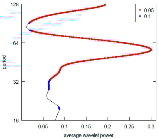
Figure 1.
Series A-AWP.
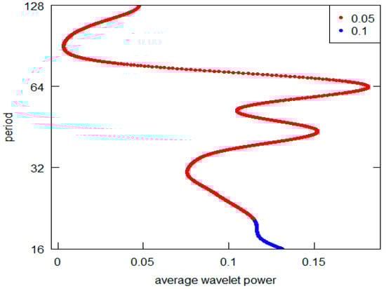
Figure 2.
Series B-AWP.
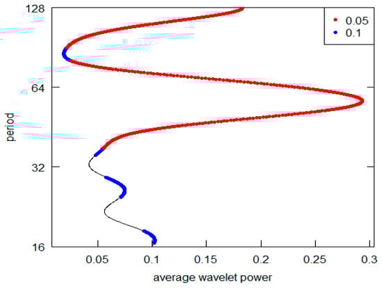
Figure 3.
Series C-AWP.
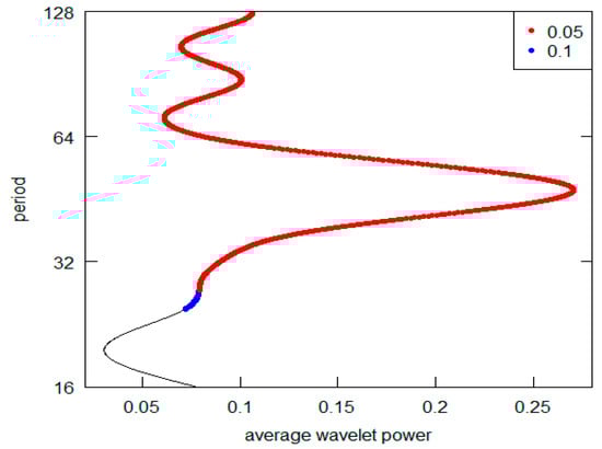
Figure 4.
Series D-AWP.
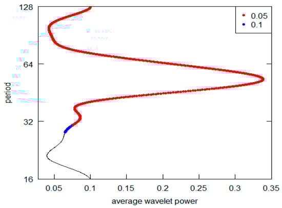
Figure 5.
Series E-AWP.
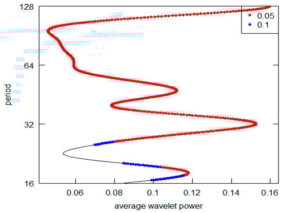
Figure 6.
Series F-AWP.
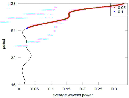
Figure 7.
Series G-AWP.
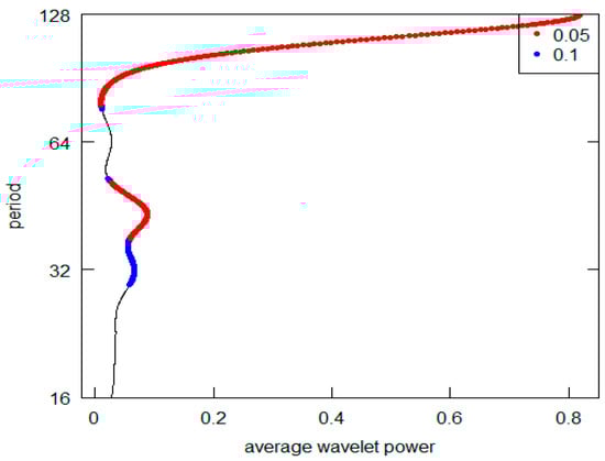
Figure 8.
Series H-AWP.
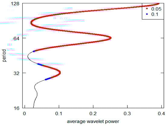
Figure 9.
Series I-AWP.
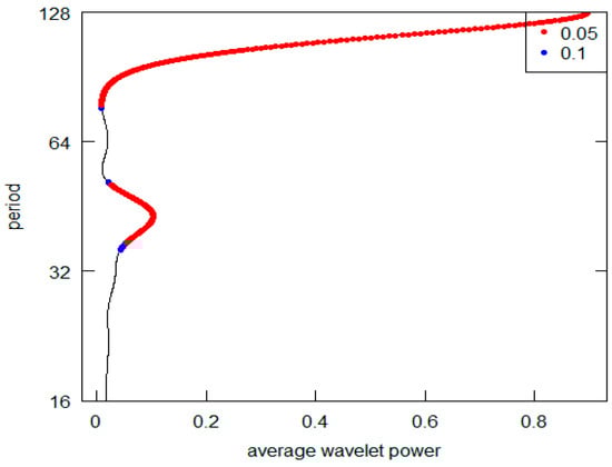
Figure 10.
Series J-AWP.
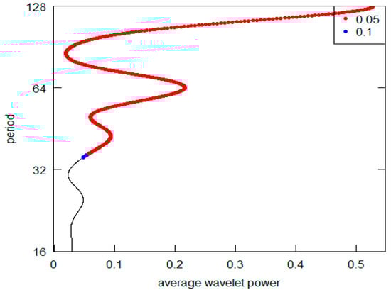
Figure 11.
Series K-AWP.
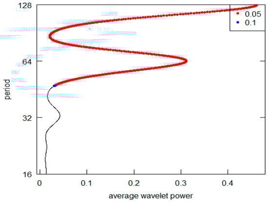
Figure 12.
Series L-AWP.
Observing this first sequence of graphs (the highest peak is represented on the vertical y-axis), it is possible to appreciate that 5 out 12 (in detail, Series A to E) reveal a periodic component in line with the K-wave hypothesis. Clearly, in all these cases, it is possible to locate the highest AWP for the period range 32–64 (the crystal scale d5). The other diagrams do not confirm this outcome. In the I, K, and L Series diagrams, the highest peak is in the d7 crystal (periodicity over the 128 years), while the second highest is at d6 crystal (period between 64 and 128). The Series G and H have the highest common peak in the d7 crystal (over 128), and, finally, the Series F and J share the d7 and the d5 crystal as the highest and second most relevant peak (over 128 and 32–64 period). The results are summarized in Table 3. For Kondratieff’s original time series, there is a majority of cases that rejects the theoretical K-wave hypothesis. As pointed out in the previous section remarking the presence of price data within this dataset, we can highlight the different types of results based on the different natures of the original data. In fact, both the series of data on prices (A, B and C) and the series of quotations (prices) of interest-bearing securities (D,E) confirm the original results achieved by Kondratieff. On the other hand, there is no confirmation from the “physical” series of consumption and production (I–L). The same rejection of the K-wave hypothesis applies to the wage series (F and G). Although we observe a coherent result for the price series, overall, we can say that our results do not confirm those of the original author. Differently, all of Kondratieff’s results were homogeneous in supporting his thesis.
Table 3.
Wavelet analysis of Kondratieff’s original data.
Moreover, and only as an example, we report in the following Figure 13, the first Kondratieff series A and its reconstruction WT using the transform. The x-axis reports the sequence of points as an index and not as chronological time (year and date) to better appreciate the duration and the flow of the swings.
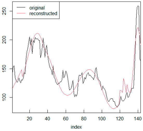
Figure 13.
Series A with WT.
The following diagrams Figure 14, Figure 15, Figure 16, Figure 17, Figure 18, Figure 19, Figure 20, Figure 21, Figure 22 and Figure 23 show the AWP for the GDP per capita series.
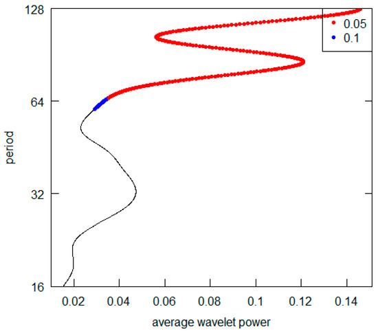
Figure 14.
Brazil GDP per capita.
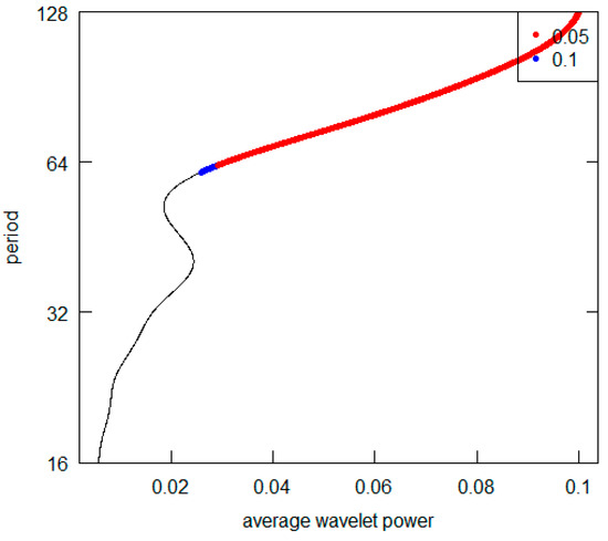
Figure 15.
France GDP per capita.
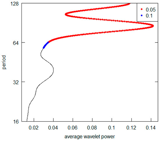
Figure 16.
Germany GDP per capita.
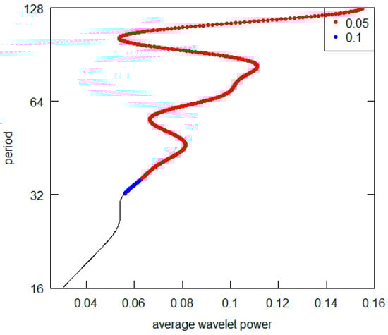
Figure 17.
India GDP per capita.
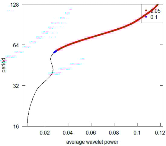
Figure 18.
Italy GDP per capita.
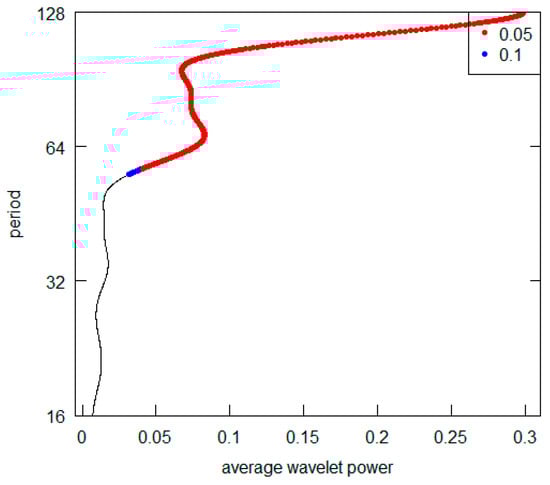
Figure 19.
Japan GDP per capita.
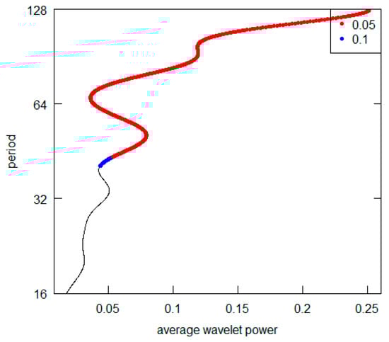
Figure 20.
Turkey GDP per capita.
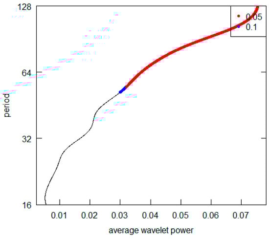
Figure 21.
United Kingdom GDP per capita.
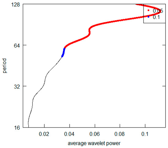
Figure 22.
United States GDP per capita.
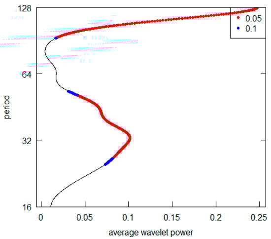
Figure 23.
Former USSR GDP per capita.
All the AWPs show that the d5 crystal is never the prevailing periodicity. For all cases (excluding the Germany and the USA), the d7 crystal represents the highest AWP peak (with a period over 128 years), while both for Germany and the USA, it is possible to note the d6 crystal (64–128 years) as the most significant one. For some countries (France, Italy and the UK) there is no second relevant periodicity in AWPs. For all those countries showing a second higher AWP peak (Brazil, Germany, India, Japan, Turkey and USSR), the most frequent periodicity is represented by the d6 crystal. All results are summarized in Table 4. Overall, from the visual inspection of the graphs, we can deduce that the long-wave hypothesis is not supported by the GDP per capita investigation. Indeed, we never detect a periodicity consistent with the hypothesis. In addition, we can point out that it is not possible to observe a common pattern across countries. Two countries (Germany and the USA) have shorter fluctuation cycles. Curiously, they are the nations with the highest total GDP in the Western World. Probably the effects of the changes that occur in their economies spread and are trasmitted with inertia to the economic systems of others countries. They play what is called “the leadership role” both internationally and within their specific areas of economic influence.
Table 4.
Wavelet analysis of GDP per capita data.
Furthermore, and only as an example, we report in the following Figure 24 and Figure 25, the series for Germany and the USA together with their WT. As previously mentioned, the x-axis reports the sequence of points as an index and not as chronological time (year and date) to better appreciate the period of the swings as shown in Table 4. The approximation of the WT with the GDP per capita series is necessarily of lower quality—than that seen in Figure 13—given its longer length (crystal d6 instead of d5).
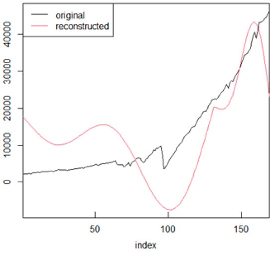
Figure 24.
Germany GDP per capita with WT.
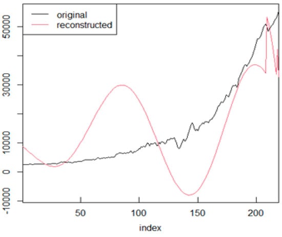
Figure 25.
USA GDP per capita with WT.
From our overall WA, we can confirm Kondratieff’s conclusions about the existence of long cycles with a period around 50 years for “his” price series. This applies to both commodities and financial securities. The more general conclusion that there are cycles of this duration for the economy as a whole, which can also be deduced from other indicators as in his original hypothesis, is not confirmed. Indeed, trying to broaden the field of investigation to the GDP per capita series, we do not find results consistent with the hypothesis. At this point, we can focus our attention and ask ourselves what might be an indicator that can best represent the overall trend of an economic system. Which indicator is the most suitable to represent the economic cycle? Prices or GDP (also in their per capita version)? The information content is quite different. From a purely financial point of view, for example, the focus of institutional investors may be more linked to the indications that can be drawn from prices. They can provide operational information for portfolio management. On the other hand (and probably), a political decision maker might be more interested in evaluating a macroeconomic indicator.
4. Conclusions
The hypothesis of the existence of periodic cycles in the economy does not conflict with the ergodic axiom of rational behavior. One may think of it as a natural consequence. This theorization is included within the literature on real business cycles. The hypothesis of the existence of alternating fluctuations within economies lasting about fifty years was first formulated by Russian economist Kondratieff. The debate on its validity is still present in the economic literature. Real shocks affecting the economy would occur, for some reason, following a definite periodicity. Furthermore, one can think of a sort of deterministic model capable of representing and predicting the ”economic future”.
Various methodologies have been proposed to investigate the existence of periodicities in economic series. One of the most powerful is the WA. This is a fairly recent technique. It has never been applied to the Kondratieff data that gave rise to the debate. We try this exercise to fill the current gap.
In this paper, firstly we propose the application of WA to Kondratieff’s original series. From our point of view, this is a necessary step, since it is from the processing of these data that this strand of economic research was born. Our investigation of this dataset confirms the long-wave hypothesis only for the price series (both commodities and interest-bearing securities). Therefore, at the same time, our findings do not confirm the entire hypothesis of Kondratieff which theorizes an alternating cycle of the economic system also through the support of coherent results in other indicators. Basically, our outcomes do not support Kondratieff’s intuition by applying the WA to his original time series. Only 5 out 12 series confirm the presence of the hypothesized periodicity.
Secondly, to broaden the perspective, we analyze longer time series of GDP per capita for different countries. If the theory is robust, it should manifest widely without special territorial and systemic limitations. We select this key macroeconomic indicator because of its importance in measuring the economic growth of a country. In this second dataset, we can observe that periodicities are different across economies and, fundamentally, there is no clear and similar pattern that is convincingly repeated. Only two out of ten countries have similar periodicities. These periodicities are lower than those found in all other cases. Interestingly, these two countries are currently considered the driving forces behind the advanced economies over which they exert the greatest influence, respectively. No case, however, is consistent with the long-wave hypothesis.
Overall, our results do not confirm Kondratieff’s hypothesis for both the original dataset and the GDP per capita series
Our empirical results provide a further contribution to the strand of literature investigating the existence of periodic business cycles and to the literature investigating the deterministic or stochastic nature of macroeconomic fluctuations. Further future research efforts can be directed towards the application of WA to prices and other macroeconomic data to test for correspondences. As we have pointed out, Kondratieff’s conclusions were not based on prices alone. Perhaps, other data can confirm this theory by suggesting a different perspective and interpretation.
Funding
This research received no external funding.
Informed Consent Statement
Not applicable.
Data Availability Statement
All data and R codes used in the study are available from the author.
Acknowledgments
The author would like to thank the Editor- and three anonymous Reviewers for their stimulating activity in improving the present manuscript.
Conflicts of Interest
The author declares no conflict of interest.
References
- Adelman, Irma. 1965. Long cycles: Fact or artifact? American Economic Review 55: 444–63. [Google Scholar]
- Aftalion, Albert. 1909. La réalité des surproductions générales: Essai d’une théorie des crises générales et périodiques. Revue d’Économie Politique XXIII: 86–87. [Google Scholar]
- Aiyagari, Sudhakar. 1994. On the contribution of technology shocks to business cycles. Federal Reserve Bank of Minneapolis Quarterly Review 18: 22–34. [Google Scholar] [CrossRef]
- Almeshari, Ali, Mohamed Hisham Bin Dato Haji Yahya, Fakarudin Bin Kamarudin, Rosalan Ali, and Sha’ari Abd Hamid. 2023. Liquidity creation, oil term of trade shocks, and growth volatility in Middle Eastern and North African Countries (MENA). Economies 11: 147. [Google Scholar] [CrossRef]
- Anguiar-Conraria, Luis, and Maria Joana Soares. 2011. Business cycles synchronization and the Euro: A wavelet analysis. Journal of Macroeconomics 33: 477–89. [Google Scholar] [CrossRef]
- Aristizabal, Felipe, and Mladen. I. Glavinovic. 2003. Wavelet analysis of nonstationary fluctuations of Monte Carlo-Simulated excitatory postsynaptic currents. Biophysical Journal 85: 2170–85. [Google Scholar] [CrossRef] [PubMed][Green Version]
- Baffigi, Alberto. 2011. Italian National Accounts, 1861–2011. Banca d’Italia Economic History Working Papers 18. Rome: Bank of Italy. [Google Scholar]
- Barro, Robert J., and José F. Ursua. 2008. Macroeconomic crises since 1870. Brooking Economic Papers on Economic Activity, Economic Studies Program 391: 255–350. [Google Scholar]
- Baxter, Marianne, and Robert King. 1999. Measuring business cycles: Approximate band-pass filters for economic time series. Review of Economic and Statistics 81: 575–93. [Google Scholar] [CrossRef]
- Beaudry, Paul, Dana Galizia, and Franck Portier. 2020. Putting the cycle back into business cycle analysis. American Economic Review 110: 1–47. [Google Scholar]
- Belkhir, Mohamed, Sami Ben Naceur, Bertrand Candelon, and Jean-Charles Wijnandts. 2022. Macroprudential policies, economic growth and banking crises. Emerging Markets Review 53: 100936. [Google Scholar] [CrossRef]
- Berry, Brian J. L. 2000. A pacemaker for the long wave. Technological Forecasting and Social Change 63: 1–23. [Google Scholar] [CrossRef]
- Berry, Brian J. L. 2006. Recurrent instabilities in K-wave macrohistory. In Kondratieff Waves, Warfare and World Security. Edited by T. C. Devezas. Amsterdam: IOS Press, pp. 22–29. [Google Scholar]
- Bieshaar, Hans, and Alfred Kleinknecht. 1984. Kondratieff long waves in aggregate output? An econometric test. Konjunkturpolitik 30: 279–303. [Google Scholar]
- Bloomfield, Peter. 2000. Fourier Analysis of Time Series—An Introduction. New York: John Wiley & Sons, Inc. [Google Scholar]
- Box, George P., Gwilym M. Jenkins, Gregory C. Reinsel, and Greta M. Ljung. 2016. Time Series Analysis-Forecasting and Control, 5th ed. Hoboken: John Wiley & Sons. [Google Scholar]
- Broadberry, Stephen, Bruce Campbell, Alexander Klein, Mark Overton, and Bas van Leewen. 2015. British Economic Growth 1278–1870. Cambridge: Cambridge University Press. [Google Scholar]
- Brock, William, Davis W. Dechert, and Blake Lebaron Jose Scheinkman. 1996. A test for independence based on the correlation dimension. Econometric Reviews 15: 197–235. [Google Scholar] [CrossRef]
- Bruce, Andrew, and HongYe Gao. 1996. Applied Wavelet Analysis with S-PLUS. New York: Springer. [Google Scholar]
- Cazelles, Bernard, Mario Chavez, Dominique Berteaux, Frédèric Ménard, Jon Olav Vik, Stéphanie Jenouvrier, and Nils C. Stenseth. 2008. Wavelet analysis of ecological time series. Oecologia 156: 287–304. [Google Scholar] [CrossRef]
- Chan, Kung-Sik, and Brian Ripley. 2022. TSA: Time Series Analysis. R Package Version 1.3.1. Available online: https://CRAN.R-project.org/package=TSA (accessed on 28 July 2023).
- Cheng, Han-Liang, and Nan-Kuang Chen. 2021. A study of financial cycles and the macroeconomy in Taiwan. Empirical Economics 61: 1749–78. [Google Scholar] [CrossRef]
- Christiano, Lawrence J., and Terry J. Fitzgerald. 2003. The band pass filter. International Economic Review 44: 435–65. [Google Scholar] [CrossRef]
- Crowley, Patrick M. 2007. A guide to wavelets for economists. Journal of Economic Surveys 21: 207–67. [Google Scholar] [CrossRef]
- Crowley, Patrick M., and Andrew H. Hallet. 2014. The great moderation under the microscope: Decomposition of macroeconomic cycles in US and UK aggregate demand. In Wavelet Applications in Economics and Finance. Edited by Marco Gallegati and Willi Semmler. Cham: Springer, pp. 47–71. [Google Scholar]
- Darné, Olivier, and Claude Diebolt. 2004. Unit roots and infrequent large shocks: New international evidence on output. Journal of Monetary Economics 51: 1449–65. [Google Scholar] [CrossRef]
- Daubechies, Ingrid. 1990. The wavelet transform time-frequency localization and signal analysis. IEEE Transactions on Information Theory 36: 961–1005. [Google Scholar] [CrossRef]
- Davidson, Paul. 2015. Post Keynesian Theory and Policy—A Realistic Analysis of the Market Oriented Capitalist Economy. Cheltenham: Edward Elgar. [Google Scholar]
- De Wolf, Salomon. 1924. Prosperitats und Depressionsperioden. In Der Lebendige Marxismus: Festgabe zum 70 Geburtstage von Karl Kautsky. Edited by Otto Jensen. Jena: Thuringer Verlagsanstalt, pp. 13–43. [Google Scholar]
- De Wolf, Salomon. 1929. Het Economisch Getij. Amsterdam: Emmering. [Google Scholar]
- Devezas, Tessaleno, and James Corredine. 2001. The biological determinants of long-wave behavior in socioeconomic growth and development. Technological Forecasting and Social Change 68: 1–57. [Google Scholar] [CrossRef]
- Diebolt, Claude. 2005. Long cycles revisited—An essay in econometric history. Economies et Sociétés 39: 23–47. [Google Scholar]
- Diebolt, Claude, and Cedric Doliger. 2006. Economic cycles under test: A spectral analysis. In Kondratieff Waves, Warfare and World Security. Edited by Tessaleno C. Devezas. Amsterdam: IOS Press, pp. 39–47. [Google Scholar]
- Focacci, Antonio. 2017. Controversial curves of the economy: An up-to-date investigation of long waves. Technological Forecasting and Social Change 116: 271–85. [Google Scholar] [CrossRef]
- Frisch, Ragnar. 1933. Propagation Problems and Impulse Problems in Dynamic Economics (in Economic Essays in Honour of Gustav Cassel, Allen & Unwin, London, pp. 171–3, 181–90, 197–203). In The Foundations of Econometric Analysis. 1995. Edited by David F. Hendry and Mary S. Morgan. Cambridge: Cambridge University Press, pp. 333–46. [Google Scholar]
- Fukao, Kyoji, Jean-Pascal Bassino, Tatsuji Makino, Ralph Paprzycki, Tokihiko Settsu, Masanori Takashima, and Joji Tokui. 2015. Regional Inequality and Industrial Structure in Japan: 1874–2008. Tokyo: Maruzen Publishing. [Google Scholar]
- Gali, Jordi. 1999. Technology, employment, and the business cycle: Do technology shocks explain aggregate fluctuations? American Economic Review 89: 249–77. [Google Scholar] [CrossRef]
- Gallegati, Marco, and Willi Semmler, eds. 2014. Wavelets Applications in Economics and Finance. Cham: Springer International Publishig. [Google Scholar]
- Gallegati, Marco, Mauro Gallegati, James B. Ramsey, and Willi Semmler. 2017. Long waves in prices: New evidence from wavelet analysis. Cliometrica 11: 127–51. [Google Scholar] [CrossRef]
- Garvy, George. 1943. Kondratieff’s theory of long cycles. The Review of Economics and Statistics 25: 203–20. [Google Scholar] [CrossRef]
- Gattei, Giorgio. 1981. I Cicli Economici Maggiori. Bologna: Nuova Casa Editrice Cappelli. [Google Scholar]
- Gençay, Ramazan, Fanuk Selçuk, and Brandon Whitcher. 2001. An Introduction to Wavelets and Other Filtering Methods in Finance and Economics. San Diego: Academic Press. [Google Scholar]
- Gerster, Hans J. 1992. Testing long waves in price and volume series from Sixteen Countries. In New Findings in Long Wave Research. Edited by Alfred Kleinknecht, Ernest Mandel and Immanuel Wallerstein. New York: St. Martin’s Press, pp. 120–47. [Google Scholar]
- Goldstein, Josha S. 1999. The existence, endogeneity and synchronization of long waves: Structural time series model estimates. Review of Radical Political Economics 31: 61–101. [Google Scholar] [CrossRef]
- Goldstein, Joshua S. 1988. Long Cycles: Prosperity and War in Modern Age. New Haven: Yale University Press. [Google Scholar]
- Gordon, Robert J. 1990. What is new-keynesian economics? Journal of Economic Literature 28: 1115–71. [Google Scholar]
- Granger, Clive W. J., and Michio Hatanaka. 1964. Spectral Analysis of Time Economic Time Series. Princeton: Princeton University Press. [Google Scholar]
- Gregory, Paul R. 1982. Russian National Income, 1885–1913. Cambridge: Cambridge University Press. [Google Scholar]
- Growiec, Jakub, Peter McAdam, and Jakub Mućk. 2018. Endogenous labor share cycles: Theory and evidence. Journal of Economic Dynamics and Control 87: 74–93. [Google Scholar] [CrossRef]
- Harkness, Jon P. 1968. A spectral-analytic test of the long-swing hypothesis in Canada. The Review of Economics and Statistics 50: 429–36. [Google Scholar] [CrossRef]
- Haustein, Heinz-Dieter, and Erich Neuwirth. 1982. Long waves in world industrial production, energy consumption, innovations, inventions, and patents and their identification by spectral analysis. Technological Forecasting and Social Change 22: 53–89. [Google Scholar] [CrossRef][Green Version]
- Hilmola, Olli-Pekka. 2007. Stock market performance and manufacturing capability of the fifth long-cycles industries. Futures 39: 393–407. [Google Scholar] [CrossRef]
- Huffaker, Rat, Marco Bittelli, and Rodolfo Rosa. 2017. Nonlinear Time Series Analysis with R. Oxford: Oxford University Press. [Google Scholar]
- Kaiser, Gerald. 2011. A Friendly Guide to Wavelets. New York: Springer. [Google Scholar]
- Kantor, Brian. 1979. Rational expectations and economic thought. Journal of Economic Literature 17: 1422–41. [Google Scholar]
- Keenan, Daniel M. 1985. A Tukey non-additivity-type test for time series nonlinearity. Biometrika 72: 39–44. [Google Scholar] [CrossRef]
- Klotz, Benjamin P., and Larry Neal. 1973. Spectral and Cross-Spectral Analysis of the Long-Swing Hypothesis. The Review of Economics and Statistics 55: 291–98. [Google Scholar] [CrossRef]
- Kondratieff, Nicolai. 1935. The Long Waves in Economic Life. The Review of Economic Statistics XVII: 105–15. [Google Scholar] [CrossRef]
- Kondratieff, Nicolai D. 1926. Die Langen Wellen der Konjunktur. Archiv für Sozialwissenschaft und Sozial Politik 56: 573–609. [Google Scholar]
- Korotayev, Andrey, and Seregy V. Tsirel. 2010. A spectral analysis of world GDP dynamics: Kondratieff waves, Kuznets swings, Juglar and Kitchin cycles in global economic development, and the 2008–2009 economic crisis. Structure and Dynamics 4: 3–57. [Google Scholar] [CrossRef]
- Li, Yuan, and Zhongjie Xie. 1999. The wavelet identification of thresholds and time delay of threshold autoregressive models. Statistica Sinica 9: 153–66. [Google Scholar]
- Lucas, Robert E., Jr. 1972. Expectations and the neutrality of money. Journal of Economic Theory 4: 103–24. [Google Scholar] [CrossRef]
- Lucas, Robert E., Jr. 1973. Some international evidence on output-inflation trade-offs. American Economic Review 63: 326–34. [Google Scholar]
- Lucas, Robert E., Jr. 1977. Understanding business cycles. In Stabilization of the Domestic and International Economy, Carnegie-Rochester Conferences on Public Policy, supplement. Edited by K. Brunner and A. H. Meltzer. Journal of Monetary Economics 5: S7–29. [Google Scholar]
- Malanima, Paolo. 2010. The long decline of a leading economy: GDP in central and northern Italy: 1300–1913. European Review of Economic History 15: 169–219. [Google Scholar] [CrossRef]
- Markevich, Andrei, and Mark Harrison. 2011. Great war: Civil war, and recovery Russia’s national income, 1913 to 1928. The Journal of Economic History 71: 672–703. [Google Scholar] [CrossRef]
- Martey Addo, Peter, Monica Billio, and Dominique Guégan. 2014. Non linear dynamics and wavelets for business cycles analysis. In Wavelets Applications in Economics and Finance. Edited by Marco Gallegati and Willi Semmler. Cham: Springer International Publishing. [Google Scholar]
- Metz, Rainer, and Winfried Stier. 1992. Modelling the long wave phenomena. Historical Social Research 17: 43–62. [Google Scholar]
- Metz, Rainer. 1992. A re-examination of long waves aggregate production series. In New Findings in Long Wave Research. Edited by Alfred Kleinknecht, Ernest Mandel and Immanuel Wallerstein. New York: St. Martin’s Press, pp. 80–119. [Google Scholar]
- Metz, Rainer. 2006. Empirical evidence and causation of Kondratieff cycles. In Kondratieff Waves, Warfare and World Security. Edited by Tessaleneo C. Devezas. Amsterdam: IOS Press, pp. 91–99. [Google Scholar]
- Metz, Rainer. 2011. Do Kondratieff waves exist? How time series techniques can help to solve the problem. Cliometrica 5: 205–38. [Google Scholar] [CrossRef]
- Minsky, Hyman P. 1992. The Financial Instability Hypothesis. Working Paper, 74. Annandale-on-Hudson: Levy Economics Institute of Bard College. [Google Scholar]
- MPD. 2020. Maddison Project Database. Available online: https://www.rug.nl/ggdc/historicaldevelopment/maddison/releases/maddison-project-database-2020?lang=en (accessed on 23 January 2023).
- Muth, Jean F. 1960. Optimal properties of exponentially weighted forecast. Journal of American Statistical Association 55: 299–306. [Google Scholar] [CrossRef]
- Muth, Jean F. 1961. Rational expectations and the theory of price movements. Econometrica 29: 315–35. [Google Scholar] [CrossRef]
- Nelson, Charles R., and Charles I. Plosser. 1982. Trends and random walks in macroeconomic time series. Journal of Monetary Economics 10: 139–62. [Google Scholar] [CrossRef]
- Percival, Donald, and Andrew Walden. 2000. Wavelets Methods for Time Series Analysis. Cambridge: Cambridge University Press. [Google Scholar]
- Petrakos, George, Konstantinos Rontos, Chiara Vavoura, and Ioannis Vavouras. 2023. The impact of recent economic crises on income inequality and the risk of poverty in Greece. Economies 11: 166. [Google Scholar] [CrossRef]
- Pigou, Arthur C. 1927. Industrial Fluctuations. London: Macmillan and Company Limited. [Google Scholar]
- Ramsey, James B. 2002. Wavelets in economics and finance: Past and future. Studies in Nonlinear Dynamics and Econometrics 6: 1–27. [Google Scholar] [CrossRef]
- Ramsey, James B., and Camille Lampard. 1998a. The decomposition of economic relationships by time scale using wavelets: Expenditure and income. Studies in Nonlinear Dynamics and Econometrics 3: 23–41. [Google Scholar] [CrossRef]
- Ramsey, James B., and Camille Lampard. 1998b. Decomposition of economic relationships by timescale using wavelets. Macroeconomic Dynamics 2: 49–71. [Google Scholar] [CrossRef]
- Rasmussen, Steel, Jan Holst, and Erik Mossekilde. 1989. Empirical investigation of economic long waves in aggregate production. European Journal of Operational Research 42: 279–93. [Google Scholar] [CrossRef]
- Reijnders, Johannes P. G. 1988. The Enigma of Long Waves. Utrecht: Drukkeru Elinkwijk BV. [Google Scholar]
- Reijnders, Johannes P. G. 1990. Long Waves in Economic Development. Aldershot: Edward Elgar. [Google Scholar]
- Reijnders, Johannes P. G. 2009. Trend movements and inverted Kondratieff waves in Dutch economy, 1800–1913. Structural Change and Economic Dynamics 20: 90–113. [Google Scholar] [CrossRef]
- Rhif, Manel, Ali Ben Abbes, Imed Riadh Farah, Beatriz Martinez, and Yanfang Sang. 2019. Wavelet transform application for/in non-stationary time series analysis: A review. Applied Sciences 9: 1345. [Google Scholar] [CrossRef]
- Ridolfi, Leonardo. 2016. The French Economy in the Long Durée. A Study on Real Wages, Working Days and Economic Performance from Louis IX to the Revolution (1250–1789). Dissertation IMT School for Advanced Studies, Lucca. Available online: http://e-theses.imtlucca.it/211/1/Ridolfi_phdthesis.pdf (accessed on 23 January 2023).
- Rösch, Angi, and Harald Schmidbauer. 2018. WaveletComp: Computational Wavelet Analysis. R Package Version 1.1. and “WaveletComp1.1: A Guided Tour through the R package” (Available in R Documentation). Available online: https://CRAN.R-project.org/package=WaveletComp (accessed on 23 January 2023).
- Schleicher, Christoph. 2002. An introduction to wavelets for economists. In Working Paper 2002–3. Ottawa: Bank of Canada. [Google Scholar]
- Schumpeter, Joseph. A. 1939. Business Cycles: A Theoretical, Historical and Statistical Analysis of the Capitalist Process. New York: McGraw-Hill Book Company. [Google Scholar]
- Silvestre, Joaquim. 1993. The market-power foundations of macroeconomic policy. Journal of Economic Literature 31: 105–41. [Google Scholar]
- Sleziak, Patrick, Kamila Hlačovă, and Jan Szolgay. 2015. Advantages of a time series analysis using wavelet transform as compared with a Fourier analysis. Slovak Journal of Civil Engineering 23: 30–36. [Google Scholar] [CrossRef]
- Slutsky, Eugen. 1927. The summation of random causes as the source of cyclic processes. Econometrica 5: 105–46. [Google Scholar] [CrossRef]
- Soper, John. C. 1975. Myth and Reality in Economic Time Series: The Long Swing Revisited. Southern Economic Journal 41: 570–79. [Google Scholar] [CrossRef]
- Sutch, Richard. 2006. National Income and Product Historical Statistics of the United States: Earliest Time to the Present. Edited by Susan B. Carter, Scott S. Gartner, Michael R. Haines, Alan Olmstead, Richard Sutch and Gavin Wright. New York: Cambridge University Press, pp. 23–25. [Google Scholar]
- Svabova, Lucia, Katarina Kramarova, and Dominika Chabadova. 2022. Impact of the COVID 19 pandemic on the business environment in Slovakia. Economies 10: 244. [Google Scholar] [CrossRef]
- Taylor, James B. 1988. Long waves in six nations: Results and speculations from a new methodology. Review IX: 373–92. [Google Scholar]
- Tong, Howell. 1978. On a threshold model. In Patterns Recognition and Signal Processing. NATO ASI Series E: Applied SC. No. 29. Edited by Chi-Hau Chen. Amsterdam: Sijthoff & Noordhoff, pp. 575–86. [Google Scholar]
- Torrence, Christofer, and Gilbert Compo. 1998. A practical guide to wavelet analysis. Bullettin of the American Meteorological Society 79: 61–78. [Google Scholar] [CrossRef]
- Trapletti, Adrian, and Kurt Hornik. 2023. tseries: Time Series Analysis and Computational Finance. R Package Version 0.10-54. Available online: https://CRAN.R-project.org/package=tseries (accessed on 1 June 2023).
- Tsoulfidis, Lefteris, and Aris Papageorgiou. 2019. The recurrence of long cycles: Theories, stylized facts and figures. World Review of Political Economy 10: 415–48. [Google Scholar] [CrossRef]
- Tsoulfidis, Lefteris, and Persefoni Tsaliki. 2022. The long recession and economic consequences of the covid-19 pandemic. Investigaciόn Econόmica 81: 3–29. [Google Scholar] [CrossRef]
- Tugan-Baranowsky, Michael. 1901. Studien zur Theorie und Geschichte der Handelskrisen in England. Jena: Scientia-Verlag. [Google Scholar]
- van Ewijk, Casper. 1982. A spectral analysis of the Kondratieff-cycle. Kyklos 35: 468–99. [Google Scholar] [CrossRef]
- van Gelderen, Jacob. 1913. Springvloed Besschouwingen over Industriéle Ontwikkeling en Prjisbeweging. Die Nieuwe Tijd 18: 254–77, 370–84, 446–64. [Google Scholar]
- Walker, James S. 2008. A Primer on Wavelets and Their Scientific Applications, 2nd ed. Boca Raton: Chapman & Hall. [Google Scholar]
- Warner, Rebecca. M. 1998. The Spectral Analysis of Time-Series Data. New York: The Guilford Press. [Google Scholar]
- Watson, Mark W. 1993. Measures of fit for calibrated models. Journal of Political Economy 101: 1011–41. [Google Scholar] [CrossRef][Green Version]
- Yule, George U. 1927. On a method of investigating periodicities in disturbed series with special reference to wolfer’s sunspot numbers. Philosophical Transactions of the Royal Society of London. Series A 226: 267–98. [Google Scholar]
Disclaimer/Publisher’s Note: The statements, opinions and data contained in all publications are solely those of the individual author(s) and contributor(s) and not of MDPI and/or the editor(s). MDPI and/or the editor(s) disclaim responsibility for any injury to people or property resulting from any ideas, methods, instructions or products referred to in the content. |
© 2023 by the author. Licensee MDPI, Basel, Switzerland. This article is an open access article distributed under the terms and conditions of the Creative Commons Attribution (CC BY) license (https://creativecommons.org/licenses/by/4.0/).