Co-Movement of Indonesian State-Owned Enterprise Stocks

Abstract

According to portfolio theory, diversifying investment to several stocks with negative correlations may reduce portfolio risk. In contrast, combining stocks with similar movement (co-movement) has no impact on portfolio risk reduction. This study aims to examine state-owned enterprise stock co-movement in Indonesia using orthogonal generalized auto-regressive conditional heteroscedasticity (O-GARCH) to help investors selectively choose stocks in a portfolio to reduce portfolio risks. Saturation sampling was used since all state-owned enterprise stocks listed on the Indonesian Stock Exchange were selected as samples. Based on monthly data from January 2013 to December 2021, the O-GARCH method was able to simplify the covariance matrix of the 17 SOEs. Of 17 SOEs, 11 had co-movement, as indicated by their similar principal components, whereas the remaining 6 stocks had a different principal component. Hence, investment managers or investors should not put the eleven stocks in the same portfolio as they have similar risk factors; instead, they may combine them with the six remaining SOE stocks which have a different co-movement. In addition, when the fiscal deficit is high and unconventional monetary policy is implemented in a crisis period, the SOE stock co-movement is higher. Thus, the SOE stock co-movement also depends on government-related matters and faces slightly different risks compared to its private-sector counterparts. Hence, the regulators formulating the policy on SOE stock holdings may use the results of this study by considering the potential merging of the SOE stocks with a similar stock return co-movement by taking account the timing in relation to fiscal deficit and crisis period.

1. Introduction

After the massive wave of privatization globally, state ownership in firms is still prevalent in many countries. Prabowo et al. (2018) state that state-owned enterprise (SOE) stocks in Europe dominate strategic industries such as utilities and electricity. Similarly, SOEs play an important role in the Indonesian economy with their business activities spread across strategic sectors, including energy, transportation, telecommunications, and banking. The number of SOEs in Indonesia is gradually decreasing (from 116, 114, 108, respectively, for the years 2018 to 2020) with the aim to even further decrease to 70 through corporate restructuring in the year 2025 (Ministry of State Owned Enterprises 2022). The average ownership of government on listed SOEs during the period 2009–2018 was 63% (Angela et al. 2019). Although state-owned enterprises continue to decrease in number, partially privatized firms in which the government holds 50–70% ownership are, on average, large in terms of total assets (Kim and Sumner 2021).

Thus, it is important to study the co-movement of stocks for state-owned enterprises since there is a trend for placing more emphasis on the roles of the SOEs in stimulating structural transformation which is followed by the design of institutions and policies (Kim and Sumner 2021). In addition, there is a declining trend in the SOEs’ share in the Indonesian capital market capitalization from 30% in the 2000s to 22.6% as of June 2021. Only three SOEs (BBRI, TLKM, BMRI) perform as the big five largest market capitalization in the Indonesian stock exchange. It means the performance of SOEs with the transformation that has been encouraged needs to improve, whether through improvements in management or adaptation to the business model. The collaboration between SOEs and the capital market is a necessity since the checks and balances of SOEs will be monitored publicly by the capital market. On the other hand, the capital market supervision will encourage improvement in SOEs’ performance. With the synergy between SOEs, the role of SOEs in the capital market is expected to increase. Therefore, a co-movement analysis is needed to carry out corporate restructuring in the framework of SOE synergy.

Various methods were applied by different studies to measure co-movement between assets and markets. However, this method is still relatively rarely used in the various research in the field of finance and investment in the Indonesian capital market. Most retail investors on the Indonesia Stock Exchange ignore the effect of stock co-movement. This is because they believe that state-owned enterprise (SOE) equities have distinct characteristics and are unrelated. In practice, each stock will tend to have a similar movement due to the same factors influencing them regardless of their characteristics. Therefore, there is a tendency to include stocks with similar driving factors in the same portfolio. The application of the O-GARCH method to predict the co-movement of shares of state-owned enterprises (SOEs) in Indonesia is important because the calculation of the variance–covariance matrix with a simple method is still a challenge for capital market players to facilitate the formulation of investment strategies for stocks in Indonesia. The application of the research findings is that it allows investors to selectively choose stocks in their investment portfolio to minimize its risk.

The objective of this study is to apply the O-GARCH method, as a simpler method for calculating the variance–covariance matrix, to predict the co-movement of shares of state-owned enterprises (SOEs) in Indonesia. Identifying the risk of a portfolio according to Markowitz portfolio theory is conducted by calculating the standard deviation of weighted-asset variance in a portfolio. The effect of combined-asset variance in assessing portfolio risk depends on its covariance. As the number of assets included in a portfolio increases, so does the variance–covariance matrix calculation which is involved. Thus, simpler methods in identifying risk such as O-GARCH in business is significant because it is time-efficient and more accurate. Based on the co-movement analysis, the active investment strategy for the SOE stock portfolio can be formulated by avoiding the inclusion of stocks that have co-movements.

In addition, with the different nature of SOEs due to government ownership and government backing in times of losses, it is important to examine the relationship between government fiscal deficit and SOE stock co-movement. Another theoretical consideration is related to the government unconventional monetary policies during crisis periods. Since the research period encompasses the COVID-19 period, the examination of unconventional monetary policies and their effect on SOE stock movement is necessary. For policymakers, especially the State Ministry of State-Owned Enterprises, the findings provide inputs for the establishment of SOE holdings for some sectors of the economy by considering the potential merging of the SOEs with similar stock return co-movement and also the relationship between fiscal deficit, unconventional monetary policy in crisis period and SOE stock co-movement. The following parts cover four sections as follows: Literature Review, Methods, Results and Discussion, and Conclusions.

2. Literature Review

2.1. Portfolio Analysis

There are several theories of stock co-movement for state-owned enterprises (SOEs) that attempt to explain the relationship between the stock prices of SOEs. State ownership theory argues that the stock prices of SOEs are influenced by the level of state ownership in the company. According to this theory, the higher the level of state ownership, the more likely it is that the stock prices of SOEs will move in the same direction. Political connections theory explains that the stock prices of SOEs are influenced by the political connections of the company. According to this theory, SOEs with strong political connections are more likely to have their stock prices move in the same direction as other SOEs with similar connections. The industry-specific factor theory indicates that the stock prices of SOEs are influenced by industry-specific factors such as market conditions, competition, and regulation. According to this theory, SOEs operating in the same industry are more likely to have their stock prices move in the same direction. Efficiency theory reveals that the stock prices of SOEs are influenced by the efficiency of the company. According to this theory, SOEs that are more efficient are more likely to have their stock prices move in the same direction as other efficient SOEs. Control rights theory highlights that the stock prices of SOEs are influenced by the control rights of the company. According to this theory, SOEs with different control rights structures are more likely to have their stock prices move in the same direction.

To study the co-movement of SOE stocks, a thorough understanding of portfolio risk and return concepts is essential since they provide the foundation to better understand the co-movement framework. The effectiveness of portfolio risk reduction according to portfolio theory is achieved through combining assets with negative correlations. This strategy will eliminate the firm-specific or idiosyncratic risk inherent in each stock. According to capital market theory, the remaining risk in a diversified portfolio is called systematic, and it is measured by beta. Based on capital asset pricing models (CAPM), the market index calculated as an input measuring beta is expected to explain all of the co-movement between two different assets (López-García et al. 2020). Following the importance of asset allocation, portfolio diversification, and the risk management field, the discussion of stock co-movement has attracted the attention of scholars in capital markets. Among much research investigating the causes, Roll (1988) reported that firm-level and market-level information determine stock co-movement. Other research by Bandyopadhyay and Ganguly (2012) stated that the factor affecting the mutual dependence or the same co-movement of firms’ stock is the economic cycle. Many firms are simultaneously affected when a country experiences a recession.

The determination of the assets included to form a portfolio is very important, because assets (such as stocks), which are interrelated and have a strong relationship with each other, are not able to generate portfolio benefits (Markowitz 1952). It would be better not to include stocks that have the same driving factors in the same portfolio, according to Robiyanto (2018). According to Bandyopadhyay and Ganguly (2012), the factor that influences the joint movement of stocks in the portfolio is the economic cycle. This factor is one of the sources of systematic risk, namely, the risk that affects all stocks in the portfolio and cannot be eliminated by diversification (Atahau 2014). In a diversified portfolio, the remaining systematic risk is measured by beta.

In its development, the portfolio analysis can be conducted using various methods, such as the Markowitz method (Markowitz 1959), single index model (Ali and Mehrotra 2008), and DCC-GARCH (El Hedi Arouri et al. 2015; Robiyanto et al. 2017). According to the portfolio theory by Markowitz (1952), reducing the risk of a portfolio depends on the correlation between the assets combined into the portfolios. To calculate risk, the covariance between the assets in the portfolio as a product of the correlation coefficient between the assets and their respective standard deviations serves as the primary determinant of portfolio risk reduction. A negative correlation is sought after, since it results in a decreasing risk. However, the cumbersome process of using correlation to minimize risk arises when dealing with many assets in a portfolio. Thus, a single index model is developed to reduce the variance–covariance matrix involved in portfolio risk assessment. Notwithstanding the ability of a single index model to reduce the number of inputs for assessing portfolio risk, the linear assumption behind the single index model may not fully reflect the patterns of risk and return relationship. Hence, the O-GARCH method is an alternative solution to simplify the process of testing risk factors that are the same across various financial instruments to generate a covariance matrix. The portfolio analysis requires a calculation of the correlation matrix and covariance between assets. A portfolio consisting of an extensive asset collection implies a more complex calculation. The O-GARCH method can be used to simplify the process of testing risk factors that are the same across various financial instruments to generate a covariance matrix. According to Bai (2011), the O-GARCH method uses principal component analysis (PCA) to summarize the variation explanatory factors in the time-series data and then uses a PCA-covariance matrix to adjust the initial data of the covariance matrix.

2.2. Co-Movement of Stocks in a Portfolio

The co-movement technique in the portfolio investment approach is based on the idea of diversification. It involves identifying assets that have low or negative correlation with each other, and constructing a portfolio that includes a mix of these assets. The theoretical approach behind this technique is based on the modern portfolio theory (MPT), which is a mathematical framework for constructing portfolios that maximizes expected return for a given level of risk, or minimizes risk for a given level of expected return. The key assumption of MPT is that investors are risk-averse and seek to maximize expected return for a given level of risk. The co-movement technique is used to achieve this by diversifying the portfolio across assets that have low or negative correlation with each other. This reduces the overall risk of the portfolio while maintaining or even increasing the expected return. The co-movement technique in the portfolio investment approach is related to several theories, including: the modern portfolio theory (MPT), the capital asset pricing model (CAPM), arbitrage pricing theory (APT), efficient market hypothesis (EMH), and behavioral finance. MPT is a mathematical framework for constructing portfolios that maximizes expected return for a given level of risk, or minimizes risk for a given level of expected return (Markowitz 1952). The co-movement technique is used to achieve this by diversifying the portfolio across assets that have low or negative correlation with each other. CAPM is a model that describes the relationship between risk and expected return for assets and portfolios. It is used to determine the cost of equity capital for a company. The co-movement technique is used in conjunction with CAPM to optimize the portfolio’s risk–return trade-off (Sharpe 1964). APT is a general theory of asset pricing that describes how the price of an asset is determined by a variety of macroeconomic factors. The co-movement technique can be used in conjunction with APT to identify assets that have low or negative correlation with each other and to construct a portfolio that is diversified across these assets (Ross 1976). EMH is an investment theory that states that financial markets are efficient and that the prices of assets reflect all the available information. The co-movement technique can be used to take advantage of market inefficiencies by identifying assets that have low or negative correlation with each other and constructing a portfolio that is diversified across these assets (Fama 1970). Behavioral finance is a field of study that looks at how psychological and social factors influence financial decisions. It is related to co-movement technique in the sense that it can help to explain why some assets are correlated and others are not, which can be useful in identifying assets that are suitable for diversification (Nofsinger 2008).

While most of the literature on portfolio theories focuses on the correlation coefficient to minimize portfolio risks, studies on the co-movement of stocks in a portfolio are also growing. The co-movement of stocks is an indicator of systematic risks in a diversified portfolio since the stocks react similarly to systemic risks factor such as inflation. Lee (2021) used ordinary least squares (OLS) quantile regression to examine the dynamic co-movement between stocks and treasury bonds in Europe. The findings showed an indication of the nonlinear effects of co-movement driving factors in the EU asset markets. To account for nonlinearity, Koulakiotis et al. (2012) applied time-varying copula models in examining a combination of the co-movement and integration effects on the volatility of cross-listed equities in Frankfurt, Zurich and Vienna. The research provides evidence on the ability of the new model to outperform the linear-based correlation (CCC-GARCH and the DCC-GARCH). The superiority of the proposed model lies in its ability to account for nonlinear and time-dependent relationships. The dynamic conditional correlation (DCC) model by Engle (2002) is a generalization of Bollerslev’s (1990) constant conditional correlation (CCC) model. DCC is effective for investigating time variations in correlations of asset returns and is able to capture the time-varying nature of the correlations and model large covariance matrices. It considers the heteroskedasticity of the return volatility and can be used to examine multiple asset returns simultaneously without adding too many parameters.

2.3. Government Deficit and Fiscal Backing

During crises, many governments experience fiscal deficit due to their attempts to directly and indirectly guarantee the losses of SOEs. Governments may choose whether to directly infuse cash to bailout problematic SOEs or provide economic stimuli to indirectly guarantee the SOEs in financial distress (Silva 2021). As a country with a high number of SOEs, the direct and indirect efforts of the Indonesian government to rescue problematic SOEs such as the Jiwasraya Insurance SOE and Garuda Indonesia Airways SOE are inevitable. The guarantee provided by the Indonesian government to its SOEs affects the magnitude of fiscal deficit. As evidenced by Silva (2021), there is a negative co-movement between economic condition and bank provision. The downturn in economic conditions increased bank provision and government guarantees which in turn widened the government fiscal deficit. Moreover, Gandhi et al. (2020) stated that when a government directly bails out SOEs, the spread in risk-adjusted returns between large and small institutions depends on the country’s characteristics that determine the likelihood of bailouts. The likelihood of an Indonesian government bailout (which affected its fiscal deficit) over the research period might have impacted the stocks’ returns to the recipients and their co-movement.

2.4. Effects of Unconventional Monetary Policies

The unconventional monetary policy implemented by the Indonesian government during the COVID-19 period was to accelerate the fiscal stimulus (budget realization) to preserve the purchasing power of society. Fiscal stimulus, especially social protection of IDR 408.7 trillion and infrastructure capital spending of IDR 417.8 trillion, supported the economic recovery from the consumption and investment side (Warjiyo 2020). Due to COVID-19, many stocks experienced far below their average past performance. In this regard, fiscal stimulus aimed to prevent further deterioration of the stocks’ performance. As a result, the sectors affected by the fiscal stimulus experienced similar movements of stock prices (co-movement). Notwithstanding the benefit, another consequence of the fiscal stimulus was the increased government deficit which reached IDR 947.7 trillion in 2020. Meanwhile, to strengthen the SOE stock capital under the impact of COVID-19, the Government provided capital to SOE in the amount of IDR 31.5 trillion. Thus, it is worthwhile examining the effect of unconventional monetary policies on SOE stocks’ co-movement.

3. Method

The monthly closing price data of SOE stocks listed on the Indonesia Stock Exchange before the COVID-19 pandemic from January 2013 to December 2021 were used. This period was selected since none of the SOEs held a seasonal equity offering through the right issue which could affect the theoretical price of a stock, thus avoiding the confounding effect. In total, there are 17 SOE stocks whose stocks were owned directly by the Indonesian Government. They are ADHI (PT Adhi Karya (Persero) Tbk), ANTM (PT Aneka Tambang (Persero) Tbk), BBNI (PT Bank Negara Indonesia (Persero) Tbk), BBRI (PT Bank Rakyat Indonesia (Persero) Tbk), BBTN (PT Bank Tabungan Negara Tbk), BMRI (PT Bank Mandiri (Persero) Tbk), INAF (PT Indo Farma (Persero) Tbk), JSMR (PT Jasa Marga (Persero) Tbk), KAEF (PT Kimia Farma (Persero) Tbk), KRAS (PT Krakatau Steel (Persero) Tbk), PGAS (PT Perusahaan Gas Negara (Persero) Tbk), PTBA (PT Bukit Asam (Persero) Tbk), PTPP (PT PP (Persero) Tbk), TINS (PT Timah (Persero) Tbk), TLKM (PT Telekomunikasi Indonesia (Persero) Tbk), WIKA (PT Wijaya Karya (Persero) Tbk), and WSKT (PT Waskita Karya (Persero) Tbk). The data were obtained from Bloomberg and the Indonesia Stock Exchange (IDX), and analyzed using orthogonal generalized autoregressive conditional heteroscedasticity (O-GARCH).

The O-GARCH method is a method that can be used to simplify the process of testing the same risk factor on various financial instruments to produce a covariance matrix, but this method is still relatively rarely used in the various available research on finance and investment in the Indonesian capital market. Luo et al. (2015) suggested that in the O-GARCH model, linearly observed time-series data should be converted to become an independent time-series data series using PCA. The O-GARCH model introduced by Alexander (2001) is as follows (adjusted for the data used in this study which uses daily data):

If Y_t is a multivariate time series of daily returns with zero average on k assets of length T with columns y_t, …, y_k. So, the matrix X_t T X K with columns x_t, …, x_k can be formulated with the equation:

$$x_t=\frac{y_t}{\sqrt{v_i}}$$

where V = diag(v₁, …, v_m), where v₁ is the sample variance of the ith column Y_t.

If L shows the eigenvector matrix of population correlation x_t and l_m = (l₁, m, …, l_k, m) is the m_th column, l_m is the eigenvector k X 1 corresponding to the eigenvalue m. The column L has been selected so that 1 > 2 > … > k. If D is a diagonal eigenvalue matrix, then the m_th principal component of the system can be expressed as:

p_m = x₁l_1,m + x₂l_2,m + … + x_kl_k,m

If each vector of the principal components pm is placed as a column in the matrix P T X k, so that:

P = XL

If the principal component column is modeled by GARCH (1,1) as suggested by Bollerslev (1990) and Engle (2002) as follows:

$$p_t|{\mathsf{\Psi }}_{t-1}~N \left(0,{\Sigma }_t\right)$$

p_i,t = ϵ_i,t

$${\sigma }_{i,t}^2={\omega }_i+{\alpha }_i{ϵ}_{i,t-1}^2+{\beta }_i{\sigma }_{i,t-1}^2$$

where Σ_t is the diagonal matrix of the conditional variance of the principal components of P. Ψ_t−1 which contains all available information up to t − 1. The Xn conditional variance matrix is D_t = LΣ_t$L_N^T$ so that the Y covariance conditional matrix is:

$$H_t=\sqrt{V}{D}_t\sqrt{V}$$

The O-GARCH method has been used by Robiyanto (2017) in measuring the degree of integration of capital markets in the ASEAN region. The O-GARCH model is the variance of the GARCH method. Some of the studies that have used the GARCH method and its variance are (1) Robiyanto (2017), who conducted research using the O-GARCH method to measure the degree of capital market integration in ASEAN member countries; (2) Robiyanto et al. (2017), who used the DCC-GARCH method to build a portfolio of stocks in Indonesia and Malaysia with gold; (3) Robiyanto (2018), who used the DCC-GARCH method to measure the dynamic correlation between stock markets in ASEAN and world oil prices; (4) Robiyanto (2018), who used the DCC-GARCH method to measure the dynamic correlation between the Indonesian stock market and the stock markets of other ASEAN countries. DCC-GARCH is able to overcome the problem of abnormal data distribution that is often found in the distribution pattern of stock returns on the Indonesian stock market. In the case of stock co-movement research, an O-GARCH application is needed because in the application of the O-GARCH model, linearly observed time-series data can be converted into an independent time-series data series using PCA (Luo et al. 2015).

The return on the SOE stocks was calculated before analyzing the data using O-GARCH. In calculating the stock price return, Gitman and Zutter (2015) was used as a reference. The formula used is as follows:

$$Retur{n}_{i,t}=(Stock Pric{e}_{i,t}-Stock Pric{e}_{i,t-1})/Stock Pric{e}_{i,t-1}$$

The O-GARCH method is best applied in a highly correlated series to examine the SOE stock price return of the banking sector (Bai 2011). The analysis was conducted using EViews 12 program. Furthermore, the method was employed since a portfolio analysis requires a calculation of the correlation matrix and covariance between assets involving a more complex calculation following the increase in the number of assets. This method is used to simplify the process of examining the same risk factors on various financial instruments to produce a covariance matrix. It combines principal component analysis (PCA) with the GARCH technique. In mathematics, PCA is often defined as a series of procedures that use orthogonal changes to simplify important information from a series of highly correlated variables to uncorrelated/low-correlated variables (Robiyanto 2017). These new orthogonal variables are then referred to as principal components (PC) and the number of PCs will be less than the number of initial variables (Bai 2011). For example, if K is the number of variables and M is the number of principal components, then M is expected to be much less than K because it is expected that noise from the data will be removed and can simplify calculations. Meanwhile, the number of principal components used in the analysis will determine the accuracy of the calculations because PCA indicates how much variation in the total of the initial data can be explained by each principal component (Alexander 2001). In general, the principal component must calculate the largest possible variance and each variance that follows has the possibility of being the highest variance by considering the constraints to be orthogonal to the previous components. The analysis was conducted using the EViews 12 program. Several studies highlighting the superiority of O-GARCH in comparison to other available methods include (Alexander 2000, 2001; Bai 2011; Klemm 2013; Robiyanto 2017). Vector autoregression (VAR) was conducted on the sample of state-owned stocks’ returns to verify the findings. The co-movement exists when the time series involved is bi-directional.

4. Results and Discussion

Table 1. Correlation of SOE stock returns listed on the Indonesia Stock Exchange (2013–2021).

	ADHI	ANTM	BBNI	BBRI	BBTN	BMRI	INAF	JSMR	KAEF	KRAS	PGAS	PTBA	PTPP	TINS	TLKM	WIKA	WSKT
ADHI	1.000000
ANTM	0.313615 0.0009	1.000000
BBNI	0.532303 0.0000	0.158441 0.1015	1.000000
BBRI	0.368020 0.0001	0.158948 0.1004	0.582553 0.0000	1.000000
BBTN	0.467890 0.0000	0.214785 0.0256	0.686145 0.0000	0.387556 0.0000	1.000000
BMRI	0.389281 0.0000	0.295527 0.0019	0.685386 0.0000	0.528003 0.0000	0.468862 0.0000	1.000000
INAF	0.039262 0.6866	0.195004 0.0431	−0.105922 0.2753	0.027085 0.7808	−0.035050 0.7188	0.000628 0.9949	1.000000
JSMR	0.448115 0.0000	0.237346 0.0134	0.597752 0.0000	0.296543 0.0018	0.455631 0.0000	0.370475 0.0001	−0.204023 0.0342	1.000000
KAEF	−0.045962 0.6367	−0.033802 0.7284	−0.286312 0.0027	−0.137166 0.1569	−0.242467 0.0115	−0.186786 0.0529	0.552909 0.0000	−0.424795 0.0000	1.000000
KRAS	0.330196 0.0005	0.545046 0.0000	0.340965 0.0003	0.168078 0.0821	0.393900 0.0000	0.389801 0.0000	0.154165 0.1112	0.245709 0.0104	0.008653 0.9292	1.000000
PGAS	0.483307 0.0000	0.426646 0.0000	0.466184 0.0000	0.232800 0.0153	0.499565 0.0000	0.401765 0.0000	0.004762 0.9610	0.423045 0.0000	−0.147053 0.1288	0.424692 0.0000	1.000000
PTBA	0.190304 0.0485	0.334188 0.0004	0.191191 0.0475	0.470570 0.0000	0.123633 0.2024	0.201589 0.0364	0.160886 0.0962	0.106741 0.2715	0.010864 0.9112	0.121924 0.2087	0.315359 0.0009	1.000000
PTPP	0.659343 0.0000	0.328962 0.0005	0.542855 0.0000	0.347135 0.0002	0.427113 0.0000	0.416511 0.0000	−0.048477 0.6183	0.489557 0.0000	−0.141505 0.1441	0.434831 0.0000	0.531963 0.0000	0.170108 0.0784	1.000000
TINS	0.379606 0.0001	0.704221 0.0000	0.304465 0.0014	0.166048 0.0859	0.388730 0.0000	0.266396 0.0053	0.101919 0.2939	0.313848 0.0009	−0.026602 0.7846	0.581455 0.0000	0.495485 0.0000	0.314486 0.0009	0.501742 0.0000	1.000000
TLKM	0.349349 0.0002	0.160480 0.0971	0.378577 0.0001	0.243984 0.0109	0.253374 0.0081	0.262524 0.0061	0.104560 0.2815	0.271188 0.0045	−0.063712 0.5124	0.135659 0.1615	0.274241 0.0041	0.033777 0.7286	0.214901 0.0255	0.095655 0.3247	1.000000
WIKA	0.707927 0.0000	0.397168 0.0000	0.558611 0.0000	0.366948 0.0001	0.408938 0.0000	0.500912 0.0000	−0.126520 0.1920	0.524985 0.0000	−0.251286 0.0087	0.405085 0.0000	0.477714 0.0000	0.230985 0.0162	0.710041 0.0000	0.400884 0.0000	0.172148 0.0748	1.000000
WSKT	0.753276 0.0000	0.471903 0.0000	0.541744 0.0000	0.369949 0.0001	0.440920 0.0000	0.377713 0.0001	−0.000736 0.9940	0.556409 0.0000	−0.174010 0.0717	0.427173 0.0000	0.539537 0.0000	0.113156 0.2436	0.651637 0.0000	0.439397 0.0000	0.258344 0.0069	0.724693 0.0000	1.000000

Source: Bloomberg, processed.

presents the correlation analysis of the SOE stock returns listed on the Indonesia Stock Exchange. The results show a significant correlation, except for the INAF and KAEF stocks which do not correlate with most of other SOE stocks. Interestingly, these stocks are from the same sector. They are the stocks of pharmacy companies owned by the state. The correlation insignificance between these stocks and other SOE stocks in the sample might relate to the anti-cyclical nature of the pharmacy sector, with a stable demand during various economic cycles, even experiencing a high increase in returns during the COVID-19 period.

Table 2. Descriptive statistics.

	ADHI	ANTM	BBNI	BBRI	BBTN	BMRI	INAF	JSMR	KAEF	KRAS	PGAS	PTBA	PTPP	TINS	TLKM	WIKA	WSKT
Mean	0.006034	0.017309	0.011013	0.005846	0.010812	0.003769	0.060439	0.001367	0.059795	0.005597	−0.002153	−0.001582	0.009851	0.011371	0.009456	0.007457	0.015890
Median	−0.011381	0.003650	0.025829	0.017271	0.009802	0.011037	−0.019344	−0.002119	−0.002075	−0.022256	−0.007748	−0.011791	0.001597	−0.006250	0.018001	−0.008135	0.005494
Maximum	0.895652	0.689956	0.302326	0.217262	0.638158	0.171717	1.410714	0.240157	4.240000	0.533898	0.491429	0.382114	0.486339	0.701987	0.232824	0.368182	0.485944
Minimum	−0.356098	−0.413251	−0.456228	−0.787013	−0.505882	−0.526119	−0.500000	−0.457265	−0.750000	−0.352174	−0.394531	−0.787500	−0.543568	−0.272523	−0.138889	−0.554667	−0.503590
Std. Dev.	0.166738	0.164000	0.100933	0.114504	0.135736	0.091356	0.339110	0.091364	0.468799	0.144511	0.135410	0.144031	0.157852	0.161818	0.063917	0.139106	0.159883
Observations	108	108	108	108	108	108	108	108	108	108	108	108	108	108	108	108	108

Source: Bloomberg, processed.

shows the descriptive statistics of SOE stocks selected as samples. ANTM, a mining company (focusing on mining coal and nickel) experienced the highest average monthly returns compared to other SOE stocks. During the research period, the commodity price worldwide showed an upward trend and made a positive impact on ANTM stock prices and returns. In contrast, PGAS had the lowest average monthly returns in comparison with other SOE stocks due to the declining trend of gas prices worldwide during the research period. Notwithstanding its lowest average monthly returns, PGAS stock movement was not as volatile as ADHI stock. Focusing on the infrastructure sector, the volatility of the ADHI monthly stock returns on average was the highest among the other infrastructure companies (WIKA and WSKT) and also of other SOE stocks. In contrast, TKLM had the lowest return volatility compared to other SOE stocks.

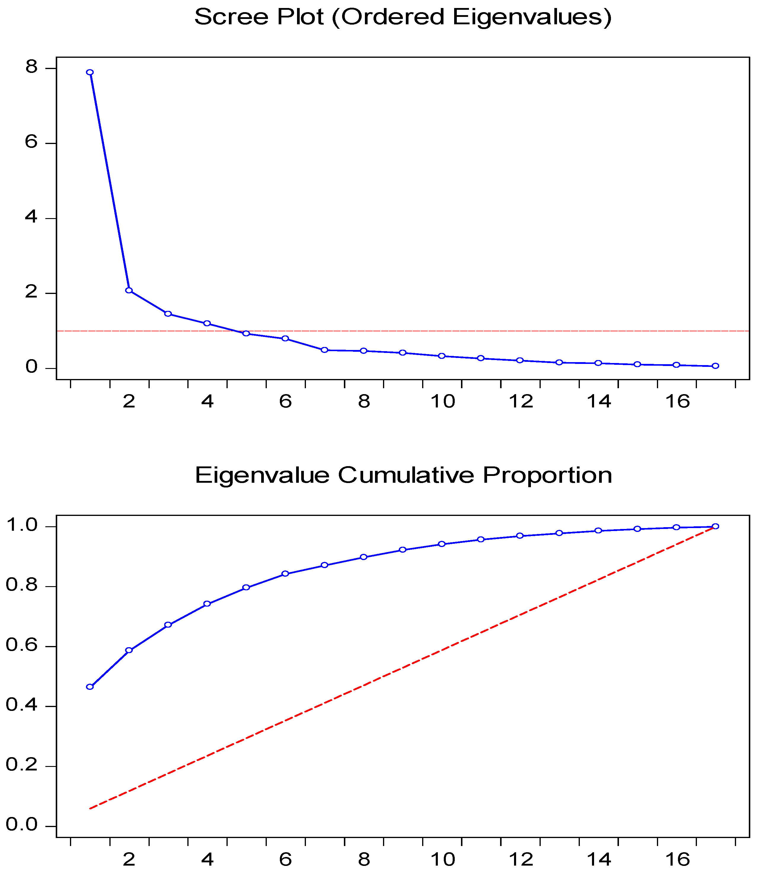
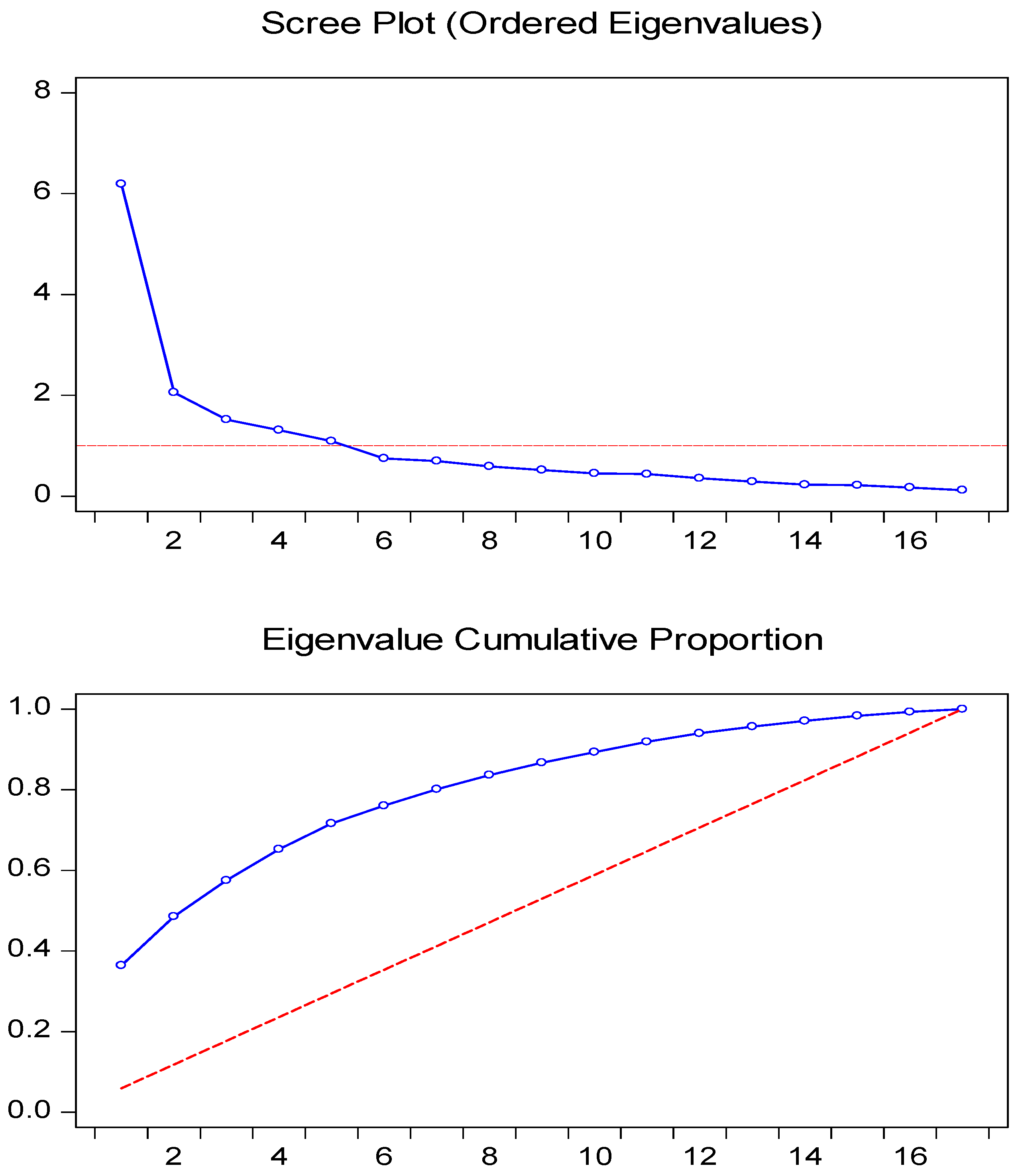
Furthermore, the results of the analysis using the O-GARCH method and PCA analysis for returns of SOE stock indicated that two main components explained the variance. The details can be seen in

Table 3. PCA analysis of SOE stock returns in the Indonesian Stock Exchange (2013–2021).

Eigenvalues: (Sum = 17, Average = 1)				Cumulative	Cumulative
Number	Value	Difference	Proportion	Value	Proportion
1	6.470491	4.413482	0.3806	6.470491	0.3806
2	2.057009	0.650215	0.1210	8.527500	0.5016

Source: Bloomberg, processed.

and

Table 4. PCA analysis for individual SOEs (2013–2021).

Variable	PC 1	PC 2
RESID_1_	0.292249	0.019560
RESID_2_	0.207784	0.393209
RESID_3_	0.317434	−0.208837
RESID_4_	0.226319	−0.076309
RESID_5_	0.274419	−0.092486
RESID_6_	0.275255	−0.073875
RESID_7_	−0.010152	0.491087
RESID_8_	0.263453	−0.234155
RESID_9_	−0.106996	0.449364
RESID_10_	0.230757	0.287781
RESID_11_	0.278888	0.100507
RESID_12_	0.134949	0.234746
RESID_13_	0.304694	0.008997
RESID_14_	0.258224	−0.123090
RESID_15_	0.241036	0.340786
RESID_16_	0.150958	−0.030183
RESID_17_	0.312665	−0.057718

Source: Bloomberg, processed.

.

Table 3 and Figure 1 show that eleven SOE stocks (ADHI, ANTM, BBNI, BBRI, BBTN, BMRI, INAF, JSMR, KAEF, KRAS and PGAS) could form PC1 with an eigenvalue of 6.470491 and a proportion of 0.3806. This means that the returns of the eleven SOE stocks had a co-movement. The first factor can explain 38.06% of the variance in the eleven stocks’ returns. Therefore, the eleven stocks had the same main risk factor and contributed 38.06% to the conditional variance of each stock. The remaining six stocks form PC2 (PTBA, PTPP, TINS, TLKM, WIKA, and WSKT) with a proportion of 12.10%. These stocks did not have the same movements and variances as the other eleven.

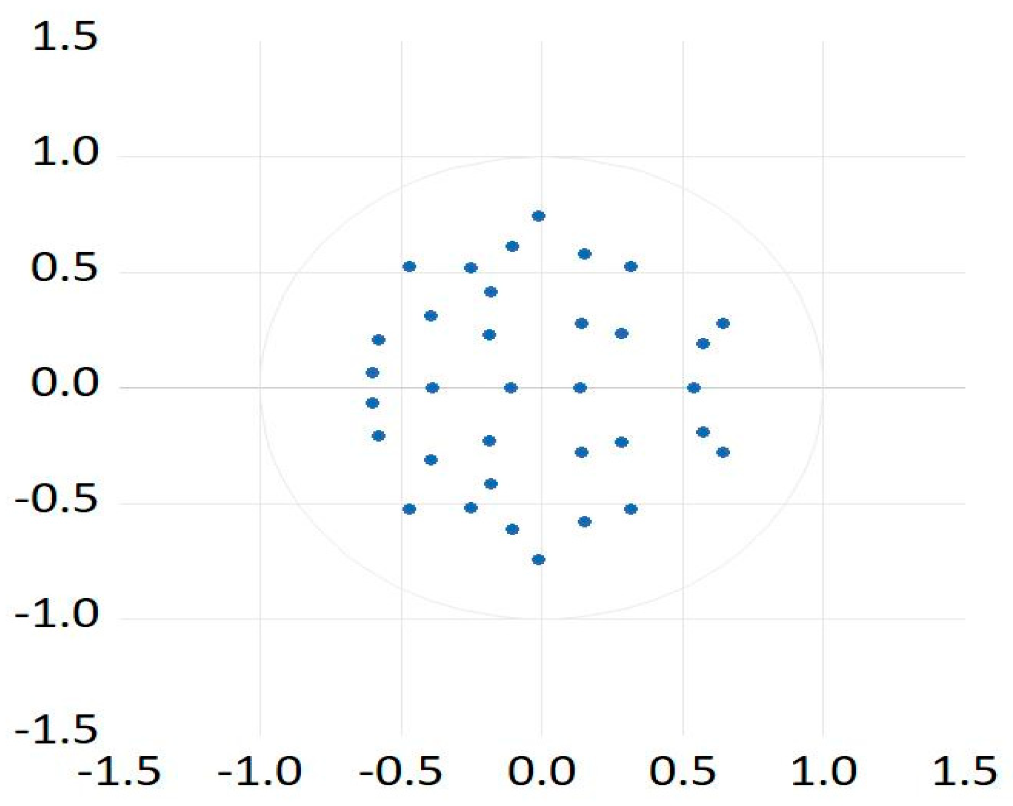
The outcomes were validated by performing a robustness analysis using the vector autoregression (VAR) stability conditions to strengthen the primary prediction.

Table 5. Vector autoregression (VAR) stability conditions.

Root	Modulus
−0.012791 + 0.741022i	0.741132
−0.012791 − 0.741022i	0.741132
0.645779 + 0.279675i	0.703739
0.645779 − 0.279675i	0.703739
−0.470491 + 0.523179i	0.703618
−0.470491 − 0.523179i	0.703618
−0.104442 + 0.613974i	0.622793
−0.104442 − 0.613974i	0.622793
−0.581872 + 0.205576i	0.617119
−0.581872 − 0.205576i	0.617119
0.317504 + 0.524267i	0.612915
0.317504 − 0.524267i	0.612915
−0.602777 − 0.064347i	0.606202
−0.602777 + 0.064347i	0.606202
0.574085 + 0.190530i	0.604876
0.574085 − 0.190530i	0.604876
0.151955 + 0.581220i	0.600755
0.151955 − 0.581220i	0.600755
−0.253564 − 0.521318i	0.579713
−0.253564 + 0.521318i	0.579713
0.540163	0.540163
−0.393135 − 0.313408i	0.502772
−0.393135 + 0.313408i	0.502772
−0.177716 + 0.416901i	0.453199
−0.177716 − 0.416901i	0.453199
−0.390063	0.390063
0.284536 − 0.237498i	0.370630
0.284536 + 0.237498i	0.370630
0.144077 + 0.278154i	0.313254
0.144077 − 0.278154i	0.313254
−0.188496 + 0.230875i	0.298050
−0.188496 − 0.230875i	0.298050
0.139023	0.139023
−0.106589	0.106589
No root lies outside the unit circle.
VAR satisfies the stability condition.

Source: Authors’ compilation.

and Figure 2 show the VAR stability conditions.

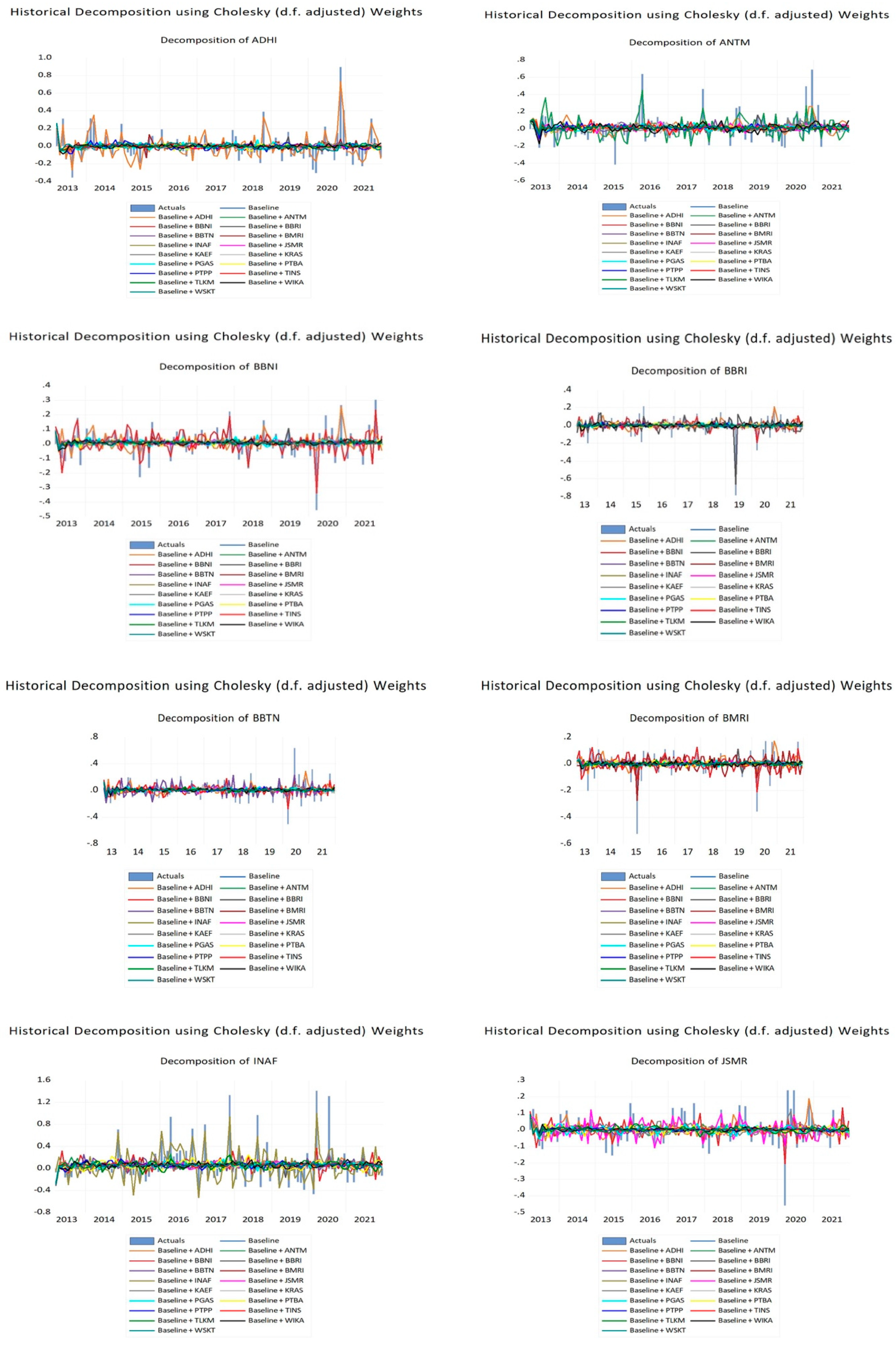
Table 5 and Figure 2 indicate that all inverse roots of the characteristic AR polynomial have a modulus less than one and lie inside the unit circle, and the estimate VAR is stable. Estimates of vector autoregression were also supported by the impulse response historical decomposition. The historical decomposition was conducted to highlight the VAR test results. The historical decomposition interprets historical fluctuations in the time-series model using the identified structural shocks as a lens. In light of the VAR, the historical decomposition summarizes the history of each endogenous variable. The historical decomposition tells us how much of the endogenous variables’ deviation from their unconditional mean is due to each shock (Figure 3).

Figure 3 reveals that almost all of the Indonesian SOE returns account for a large part of fluctuation (shock) since the beginning of COVID-19 pandemic (particularly in March, 2020). Overall, the results of the historical decomposition indicate that the greater magnitude of shock comes from themselves. The findings of this study concluded that the hypothesis was supported empirically. The orthogonal-GARCH method can predict the co-movement of the state-owned stocks in Indonesia. It summarizes the covariance matrix to be simplified for further application to facilitate the portfolio calculation. As stated by Paolella et al. (2021), the OGARCH model is suitable for a specified number of leading principal components of the covariance matrix, and the results are consistent with the findings of Byström (2004), Robiyanto (2017), and De la Torre Torres (2013).

It is also quite interesting that the rest of 49.84% of the conditional variance return of the seventeen stocks studied could be explained by other components outside this study. Therefore, there were undetectable and random factors that could affect the conditional variance return of the four analyzed stocks. Within the capital asset pricing model (CAPM) framework, this finding proves that 50.16% of the risk is systematic, while the remaining 49.84% is non-systematic.

The co-movement technique in the portfolio investment approach is based on the idea of diversification, which aims to reduce the overall risk of a portfolio by including a mix of assets that have low or negative correlation with each other. The general theory behind this is that when assets are uncorrelated or negatively correlated, the risk associated with one asset will not necessarily affect the performance of the other assets in the portfolio. When it comes to “what should” the co-movement be based on, it depends on the specific investment strategy and the type of assets included in the portfolio. In general, the co-movement should be based on the historical correlation between the assets in the portfolio, as well as any other factors that may influence the correlation, such as economic conditions and market trends. As for “why should” the co-movement be based on general theory, it is because diversifying a portfolio in this way can help to reduce the overall risk of the portfolio while maintaining or even increasing the expected return. By including a mix of assets that have low or negative correlation with each other, the portfolio is less likely to be affected by the performance of any single asset. This can lead to more stable returns over time and can help to protect the portfolio from market downturns. In addition to this, it can also help to identify new opportunities for investment that may not be apparent when looking at individual assets in isolation. By considering the correlation between assets, it may be possible to identify assets that have low or negative correlation with each other, and that may therefore be suitable for inclusion in the portfolio.

Based on these arguments, it is justifiable that the findings provide empirical evidence for the modern portfolio theory and CAPM. The co-movement from the perspective of modern portfolio theory is used to achieve minimized risk for a given level of expected return and it was achieved by diversifying the portfolio across assets that have low or negative correlation with each other (Markowitz 1952). In other words, avoiding combining stocks with similar movement (co-movement of stocks) in the same portfolio, thus leaving the systematic risk as implied by CAPM. In general, markets with low correlation tend to have higher diversification benefits due to a higher dispersion of risk (Atahau 2014; Atahau et al. 2022; Bandyopadhyay and Ganguly 2012; Jiang et al. 2017; Markowitz 1952; Robiyanto 2018).

4.1. SOE Stock Co-Movement, Government Deficit and Fiscal Backing

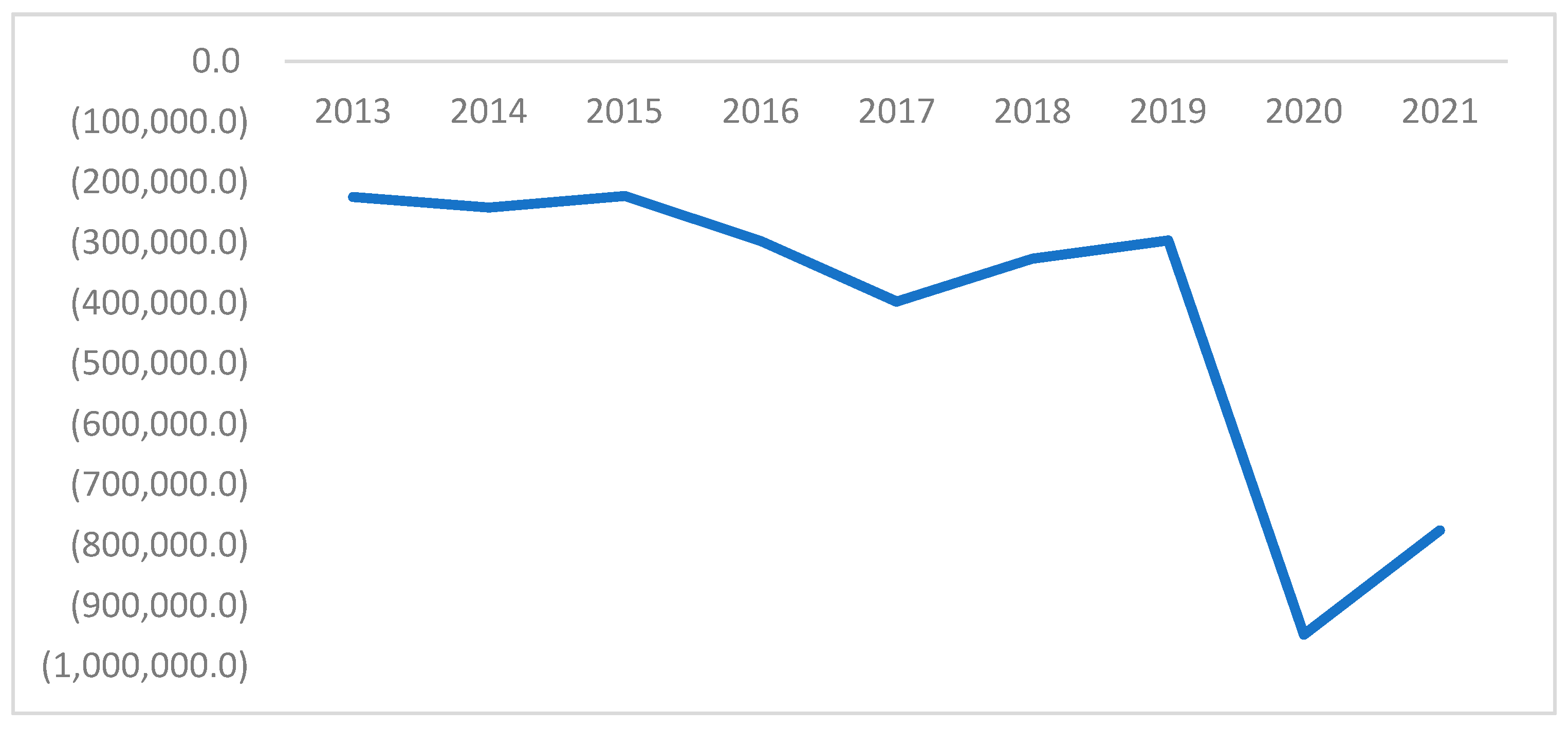
The analysis of the fiscal policy impact on SOE stock co-movement was also examined. An increase in government fiscal deficits might reduce the financial backing provided by the government to SOEs (Benmelech and Tzur-Ilan 2020; Silva 2021). The Indonesian government fiscal deficit during the research period is shown below in Figure 4.

Based on Figure 4, the median appears in 2016. It means the years with lower than median government fiscal deficit is classified as low government fiscal deficit and vice versa. According to Silva (2021), government deficits represent an important state variable indicating the credibility and strength of government guarantees. The strength of government guarantees can be an important determinant of state-owned stock co-movement (Haddad et al. 2021; Silva 2021). If a government is financially constrained (high deficits), one would expect that the co-movement of state-owned enterprises would be critically relevant (higher co-movement). The impact of low and high government fiscal deficit periods on SOE stocks’ co-movement eigenvalues is depicted in Figure 5 and Figure 6. The PCA analysis of the low government fiscal deficit period is also shown in

Table 6. PCA analysis of SOE stock returns in the Indonesian Stock Exchange in low government fiscal deficit period.

Eigenvalues: (Sum = 17, Average = 1)				Cumulative	Cumulative
Number	Value	Difference	Proportion	Value	Proportion
1	5.298803	2.889017	0.3117	5.298803	0.3117
2	2.409786	0.759474	0.1418	7.708588	0.4534

Source: Bloomberg, processed.

and

Table 7. PCA analysis for individual SOEs in low government fiscal deficit period.

Variable	PC 1	PC 2
RESID_1_	0.295224	−0.217548
RESID_2_	0.176548	0.406269
RESID_3_	0.330173	−0.167910
RESID_4_	0.308908	−0.217546
RESID_5_	0.269093	−0.014685
RESID_6_	0.313940	−0.012945
RESID_7_	0.171985	0.340620
RESID_8_	0.228022	−0.169721
RESID_9_	0.216653	0.106345
RESID_10_	0.178561	0.411516
RESID_11_	0.203844	0.025242
RESID_12_	0.140588	0.350630
RESID_13_	0.202784	−0.013452
RESID_14_	0.158342	0.427432
RESID_15_	0.183691	−0.181587
RESID_16_	0.325673	−0.066192
RESID_17_	0.280275	−0.205962

Source: Bloomberg, processed.

. During this period, 12 stocks (ADHI, BBNI, BBRI, BBTN, BMRI, JSMR, KAEF, PGAS, PTPP, TLKM, WIKA, and WSKT) formed PC1 with an eigenvalue of 5.298803 and a proportion of 0.3117. This means that the returns of the twelve SOE stocks had a co-movement. The first factor can explain 31.17% of the variance in the twelve stocks’ returns. These twelve stocks had the same main risk factor and contributed 31.17% to the conditional variance of each stock. The remaining five stocks formed PC2 (ANTM, INAF, KRAS, PTBA, and TINS) with a proportion of 14.18%. These stocks did not have the same movements and variances as the other twelve.

The PCA analysis in the high government fiscal deficit period shown in

Table 8. PCA analysis of SOE stock returns in the Indonesian Stock Exchange in high government fiscal deficit period.

Eigenvalues: (Sum = 17, Average = 1)				Cumulative	Cumulative
Number	Value	Difference	Proportion	Value	Proportion
1	7.891659	5.820632	0.4642	7.891659	0.4642
2	2.071027	0.620825	0.1218	9.962686	0.5860

Source: Bloomberg, processed.

and

Table 9. PCA analysis for individual SOEs in high government fiscal deficit period.

Variable	PC 1	PC 2
RESID_1_	0.283149	0.115282
RESID_2_	0.221851	0.362051
RESID_3_	0.286842	−0.221544
RESID_4_	0.176609	−0.008573
RESID_5_	0.252398	−0.143193
RESID_6_	0.263636	−0.173633
RESID_7_	−0.055365	0.485315
RESID_8_	0.256283	−0.247205
RESID_9_	−0.152257	0.516000
RESID_10_	0.254182	0.150741
RESID_11_	0.281636	0.130593
RESID_12_	0.117282	0.226231
RESID_13_	0.319821	0.033010
RESID_14_	0.254444	0.297575
RESID_15_	0.135863	0.036557
RESID_16_	0.294798	−0.059653
RESID_17_	0.319262	0.086204

Source: Bloomberg, processed.

was slightly different from the low deficit period. In the high deficit period, 12 stocks (ADHI, BBNI, BBRI, BBTN, BMRI, JSMR, KRAS, PGAS, PTPP, TLKM, WIKA, and WSKT) formed PC1 with an eigenvalue of 5.820632 and a proportion of 0.4642. This means that the returns of the twelve SOE stocks had a stronger co-movement than in the low deficit period. The first factor can explain 46.42% of the variance in the twelve stocks’ returns. These twelve stocks had the same main risk factor and contributed 46.42% to the conditional variance of each stock. The remaining five stocks formed PC2 (ANTM, INAF, KAEF, PTBA, and TINS) with a proportion of 12.18%. These stocks did not have the same movements and variances as the other twelve.

Based on the comparison of SOE stock co-movement between low and high government fiscal deficit, it is clear that the SOE stock co–movement was different when the government fiscal deficit was high compared to the situation when the government fiscal deficit was low. The co-movement of SOE stocks was higher (as indicated by its contribution to the conditional variance) when the government experienced a higher fiscal deficit. This is in line with the statement of Haddad et al. (2021) and Silva (2021).

4.2. Effects of Unconventional Monetary Policy Due to COVID-19 Pandemic

The Indonesian government’s unconventional monetary policy (other than interest rate policy) during the COVID-19 period was in the form of fiscal stimulus aimed to prevent further deterioration of stock performance. As a result, the sectors affected by the fiscal stimulus experienced a similar movement of stock prices (co-movement). The impact of the COVID-19 period on SOE stocks’ co-movement eigenvalues is depicted in Figure 7 and Figure 8. The PCA analysis in the pre-COVID-19 period is shown in

Table 10. PCA analysis of SOE stock returns in the Indonesian Stock Exchange in pre-COVID-19 period.

Eigenvalues: (Sum = 17, Average = 1)				Cumulative	Cumulative
Number	Value	Difference	Proportion	Value	Proportion
1	6.190520	4.132952	0.3641	6.190520	0.3641
2	2.057568	0.536677	0.1210	8.248088	0.4852

Source: Bloomberg, processed.

and

Table 11. PCA analysis for individual SOEs in pre-COVID-19 period.

Variable	PC 1	PC 2
RESID_1_	0.289265	−0.004573
RESID_2_	0.202793	0.435285
RESID_3_	0.315074	−0.230960
RESID_4_	0.219415	−0.110253
RESID_5_	0.265368	−0.185721
RESID_6_	0.282501	−0.108088
RESID_7_	−0.039741	0.410545
RESID_8_	0.272097	−0.217857
RESID_9_	−0.160905	0.359053
RESID_10_	0.219134	0.334752
RESID_11_	0.243954	0.150511
RESID_12_	0.116975	0.275000
RESID_13_	0.293614	0.015704
RESID_14_	0.218168	0.371260
RESID_15_	0.110352	−0.069534
RESID_16_	0.327631	−0.012436
RESID_17_	0.318606	0.022272

Source: Bloomberg, processed.

. In this pre-COVID-19 period, 11 stocks (ADHI, BBNI, BBRI, BBTN, BMRI, JSMR, PGAS, PTPP, TLKM, WIKA, and WSKT) formed PC1 with an eigenvalue of 6.1190520 and a proportion of 0.3641. The first factor can explain 36.41% of the variance in the eleven stocks’ returns. These eleven stocks had the same main risk factor and contributed 36.41% to the conditional variance of each stock. The remaining six stocks formed PC2 (ANTM, INAF, KAEF, KRAS, PTBA, and TINS) with a proportion of 12.18%. These stocks did not have the same movements and variances as the other eleven.

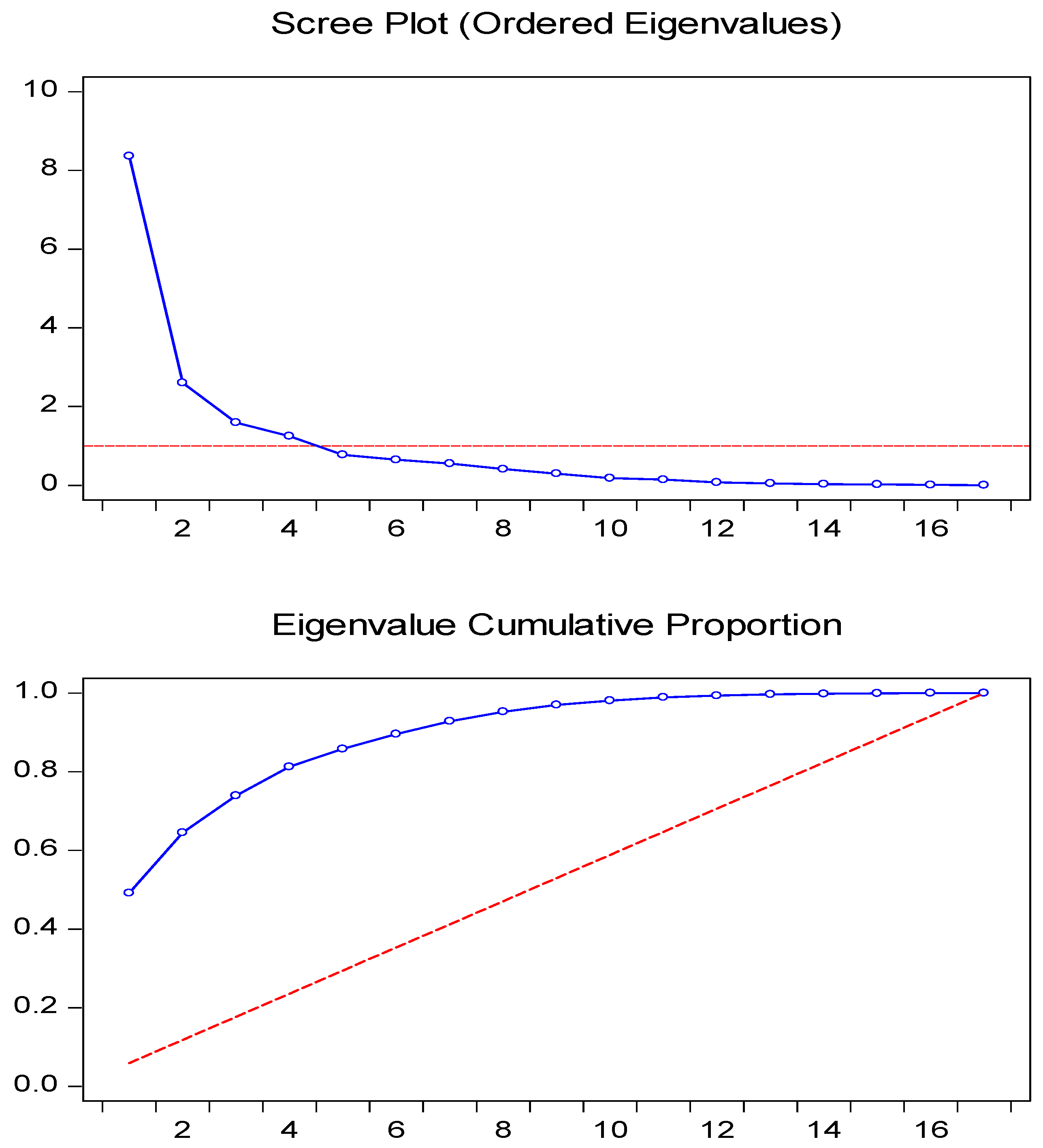
The PCA analysis during the COVID-19 period is shown in

Table 12. PCA analysis of SOE stock returns in the Indonesian Stock Exchange during COVID-19 period.

Eigenvalues: (Sum = 17, Average = 1)				Cumulative	Cumulative
Number	Value	Difference	Proportion	Value	Proportion
1	8.363124	5.759418	0.4919	8.363124	0.4919
2	2.603707	1.010807	0.1532	10.96683	0.6451

Source: Bloomberg, processed.

and

Table 13. PCA analysis for individual SOEs during COVID-19 period.

Variable	PC 1	PC 2
RESID_1_	0.297001	−0.153388
RESID_2_	0.206096	0.238408
RESID_3_	0.272358	−0.122763
RESID_4_	0.240708	0.039489
RESID_5_	0.250194	0.021791
RESID_6_	0.210498	0.214148
RESID_7_	0.074125	0.542905
RESID_8_	0.212315	−0.291630
RESID_9_	0.094947	0.531788
RESID_10_	0.217243	0.220929
RESID_11_	0.320868	−0.016399
RESID_12_	0.181382	−0.152952
RESID_13_	0.316393	−0.075517
RESID_14_	0.276926	0.212988
RESID_15_	0.208129	−0.189226
RESID_16_	0.286624	−0.173320
RESID_17_	0.292213	−0.068488

Source: Bloomberg, processed.

. During the COVID-19 period, 13 stocks (ADHI, BBNI, BBRI, BBTN, INAF, JSMR, PGAS, PTBA, PTPP, TINS, TLKM, WIKA, and WSKT) formed PC1 with a higher eigenvalue of 8.363124 and proportion of 0.4919 than the pre-COVID-19 period. The COVID-19 period had a much higher proportion. The first factor can explain 49.19% of the variance in the thirteen stocks’ returns. These thirteen stocks had the same main risk factor and contributed 49.19% to the conditional variance of each stock. The remaining four stocks formed PC2 (ANTM, BMRI, KAEF, and KRAS) with a proportion of 15.32%. These stocks did not have the same movements and variances as the other thirteen.

Based on the comparison of SOE stock co-movement during the pre-COVID-19 period and the COVID-19 period, it is clear that the SOE stock co-movement was different in the pre-COVID-19 period compared to the COVID-19 period. The co-movement of SOE stocks was higher (as indicated by its contribution to the conditional variance) during the COVID-19 period. The findings imply that there is an effect from unconventional monetary policies that consequently affects stock co-movement in Indonesia. During the COVID-19 period, several central banks of advanced economies and emerging markets announced a series of quantitative easing policies (Cortes et al. 2020). Based on Cortes et al. (2020) and Haddad et al. (2021), the Indonesian monetary authority announced unconventional monetary policies on April 1, 2020 which were associated with a variety of market effects (Cortes et al. 2020; Hattori et al. 2016). This was similar to the policy of governments around the world that also announced expansionary fiscal policies to weather the effects of the pandemic (Benmelech and Tzur-Ilan 2020).

5. Conclusions

The objective of this study was to apply the O-GARCH method to predict the co-movement of stocks of state-owned enterprises (SOEs) in Indonesia. The O-GARCH method could simplify the covariance matrix of the four SOE stocks examined. The findings showed that 11 (ADHI, ANTM, BBNI, BBRI, BBTN, BMRI, INAF, JSMR, KAEF, KRAS and PGAS) of the 17 SOE stocks analyzed using the O-GARCH method had co-movement as indicated by their similar principal components, whereas the remaining 6 stocks (PTBA, PTPP, TINS, TLKM, WIKA, and WSKT) had a different principal component.

In addition, an examination of the relationship between government fiscal deficit and SOE stock co-movement showed that the co-movement of SOE stocks was higher (as indicated by its contribution to the conditional variance) when the government experienced a higher fiscal deficit. The findings provide empirical evidence for the underlying theory related to the different nature of SOEs in government ownership which receive government backing with government fiscal deficit and reflect the government capacity to support SOEs.

Another theoretical consideration is related to the unconventional monetary policies of government during crisis periods. The examination of unconventional monetary policies and their effect on SOE stock movement showed that the SOE stock co-movement was different in the pre-COVID-19 period compared to the COVID-19 period. The co-movement of SOE stocks was higher (as indicated by their contribution to the conditional variance) during the COVID-19 period. The findings imply that there is an effect from unconventional monetary policies that consequently affects stock co-movement in Indonesia.

The findings imply that investment managers or investors should not put the eleven stocks in the same portfolio as they have similar risk factors. The other six stocks can be combined with other SOE stocks. Consequently, evaluating the co-movement of SOE stocks when designing a portfolio is essential for minimizing risk. The regulators formulating the policy on SOE-stock holding may use the results of this study by considering the potential of merging the SOE stocks with similar stock return co-movement. In times when the fiscal deficit is high and unconventional monetary policy is implemented, such as in a period of crisis, the SOE stock co-movement is higher. Thus, SOE stock co-movement also depends on government-related matters and faces slightly different risks compared to its private-sector counterparts. Future studies should be conducted on different time periods to capture the impact as the factors causing stock co-movement. The results can be used to form optimal portfolios, considering the important role of the SOE in the Indonesian economy.

References

- Alexander, Carol. 2000. A Primer on the Orthogonal GARCH Model. ISMA Centre Working Paper. Reading: ISMA Centre. [Google Scholar]
- Alexander, Carol. 2001. Orthogonal GARCH. New York: Prentice-Hall. [Google Scholar]
- Ali, Yansen, and Sanjay Mehrotra. 2008. Simplifying the Portfolio Optimization Process via Single Index Model. Novanston: Northwestern University. [Google Scholar]
- Angela, Jessica, Marcelia Jessica, Rinaningsih Rinaningsih, and Luciana Haryono. 2019. Pengaruh Kepemilikan Pemerintah Terhadap Kinerja Perusahaan Badan Usaha Milik Negara Yang Terdaftar Di BEI. Studi Akuntansi dan Keuangan Indonesia 2: 203–23. [Google Scholar] [CrossRef]
- Atahau, Apriani Dorkas Rambu. 2014. Loan Portfolio Structures, Risk and Performance of Different Bank Ownership Types: An Indonesian Case. Perth: Curtin University. [Google Scholar]
- Atahau, Apriani Dorkas Rambu, Robiyanto Robiyanto, and Andrian Dolfriandra Huruta. 2022. Predicting Co-Movement of Banking Stocks Using Orthogonal GARCH. Risks 10: 158. [Google Scholar] [CrossRef]
- Bai, Jingjing. 2011. Using Orthogonal GARCH to Forecast Covariance Matrix of Stock Returns. Houston: University of Houston. [Google Scholar]
- Bandyopadhyay, Arindam, and Sonali Ganguly. 2012. Empirical Estimation of Default and Asset Correlation of Large Corporates and Banks in India. Journal of Risk Finance 14: 87–99. [Google Scholar] [CrossRef]
- Benmelech, Efraim, and Nitzan Tzur-Ilan. 2020. The Determinants of Fiscal and Monetary Policies during the COVID-19 Crisis. NBER Working Paper Series. Cambridge: NBER. [Google Scholar]
- Bollerslev, Tim. 1990. Modelling the Coherence in Short-Run Nominal Exchange Rates: A Multivariate Generalized Arch Model. The Review of Economics and Statistics 72: 498–505. [Google Scholar] [CrossRef]
- Byström, Hans N. E. 2004. Orthogonal GARCH and Coariance Matrix Forecasting: The Nordic Stock Markets during the Asian Financial Crisis 1997–1998. European Journal of Finance 10: 44–67. [Google Scholar] [CrossRef]
- Cortes, Gustavo S., George P. Gao, Felipe B. G. Silva, and Zhaogang Song. 2020. Unconventional Monetary Policy and Disaster Risk: Evidence from the Subprime and COVID–19 Crises. Journal of International Money and Finance 122: 102543. [Google Scholar] [CrossRef]
- De la Torre Torres, Oscar. 2013. Orthogonal GARCH Matrixes in the Active Portfolio Management of Defined Benefit Pension Plans: A Test for Michoacán. Economía Teoría y Práctica 39: 119–44. [Google Scholar] [CrossRef]
- El Hedi Arouri, Mohamed, Amine Lahiani, and Duc Khuong Nguyen. 2015. World Gold Prices and Stock Returns in China: Insights for Hedging and Diversification Strategies. Economic Modelling 44: 273–82. [Google Scholar] [CrossRef]
- Engle, Robert. 2002. Dynamic Conditional Correlation: A Simple Class of Multivariate Generalized Autoregressive Conditional Heteroskedasticity Models. Journal of Business & Economic Statistics 20: 339–50. [Google Scholar]
- Fama, Eugene Francis. 1970. Efficient Capital Markets: A Review of Theory and Empirical Work. The Journal of Finance 25: 383–417. Available online: http://www.jstor.org/stable/2325486 (accessed on 20 November 2022).
- Gandhi, Priyank, Hanno Lustig, and Alberto Plazzi. 2020. Equity Is Cheap for Large Financial Institutions. Review of Financial Studies 33: 4231–71. [Google Scholar] [CrossRef]
- Gitman, Lawrence J., and Chad J. Zutter. 2015. Principles of Managerial Finance, 14th ed. London: Pearson. [Google Scholar]
- Haddad, Valentin, Alan Moreira, and Tyler Muir. 2021. When Selling Becomes Viral: Disruptions in Debt Markets in the COVID-19 Crisis and the Fed’s Response. Review of Financial Studies 34: 5309–51. [Google Scholar] [CrossRef]
- Hattori, Masazumi, Andreas Schrimpf, and Vladyslav Sushko. 2016. The Response of Tail Risk Perceptions to Unconventional Monetary Policy. American Economic Journal: Macroeconomics 8: 111–36. [Google Scholar] [CrossRef]
- Jiang, Yonghong, He Nie, and Joe Yohanes Monginsidi. 2017. Co-Movement of ASEAN Stock Markets: New Evidence from Wavelet and VMD-Based Copula Tests. Economic Modelling 64: 384–98. [Google Scholar] [CrossRef]
- Kim, Kyunghoon, and Andy Sumner. 2021. Bringing State-Owned Entities Back into the Industrial Policy Debate: The Case of Indonesia. Structural Change and Economic Dynamics 59: 496–509. [Google Scholar] [CrossRef]
- Klemm, Alexander. 2013. Growth Following Investment and Consumption-Driven Current Account Crises. Available online: https://www.imf.org/external/pubs/ft/wp/2013/wp13217.pdf (accessed on 20 November 2022).
- Koulakiotis, Athanasios, Nikos Kartalis, Katerina Lyroudi, and Nicholas Papasyriopoulos. 2012. Asymmetric and Threshold Effects on Comovements among Germanic Cross-Listed Equities. International Review of Economics and Finance 24: 327–42. [Google Scholar] [CrossRef]
- Lee, Hyunchul. 2021. Time-Varying Comovement of Stock and Treasury Bond Markets in Europe: A Quantile Regression Approach. International Review of Economics and Finance 75: 1–20. [Google Scholar] [CrossRef]
- López-García, María Nieves, Miguel Angel Sánchez-Granero, Juan Evangelista Trinidad-Segovia, Antonio Manuel Puertas, and Francisco Javier De las Nieves. 2020. A New Look on Financial Markets Co-Movement through Cooperative Dynamics in Many-Body Physics. Entropy 22: 954. [Google Scholar] [CrossRef]
- Luo, Cuicui, Luis Seco, and Lin Liang Bill Wu. 2015. Portfolio Optimization in Hedge Funds by OGARCH and Markov Switching Model. Omega 57: 34–39. [Google Scholar] [CrossRef]
- Markowitz, Harry Max. 1952. Portfolio Selection. The Journal of Finance 7: 77–91. [Google Scholar] [CrossRef]
- Markowitz, Harry Max. 1959. Portfolio Selection: Efficient Diversification of Investments. London: Yale University Press. [Google Scholar]
- Ministry of State Owned Enterprises. 2022. Portfolio Overview. Jakarta Pusat: Kementerian Badan Usaha Milik Negara. [Google Scholar]
- Nofsinger, John. 2008. The Psychology of Investing, 3rd ed. Upper Saddle River: Pearson/Prentice Hall. [Google Scholar]
- Paolella, Marc S., Paweł Polak, and Patrick S. Walker. 2021. A Non-Elliptical Orthogonal GARCH Model for Portfolio Selection under Transaction Costs. Journal of Banking and Finance 125: 106046. [Google Scholar] [CrossRef]
- Prabowo, Ronny, Reggy Hooghiemstra, and Paula Van Veen-Dirks. 2018. State Ownership, Socio-Political Factors, and Labor Cost Stickiness. European Accounting Review 27: 771–96. [Google Scholar] [CrossRef]
- Robiyanto, Robiyanto. 2017. The Analysis of Capital Market Integration in Asean Region by Using the OGARCH Approach. Jurnal Keuangan dan Perbankan 21: 169–75. [Google Scholar] [CrossRef]
- Robiyanto, Robiyanto. 2018. DCC-GARCH Application in Formulating Dynamic Portfolio between Stocks in the Indonesia Stock Exchange with Gold. Indonesian Capital Market Review 10: 13–23. [Google Scholar] [CrossRef]
- Robiyanto, Robiyanto, Sugeng Wahyudi, and Irene Rini Demi Pangestuti. 2017. The Volatility–Variability Hypotheses Testing and Hedging Effectiveness of Precious Metals for the Indonesian and Malaysian Capital Markets. Gadjah Mada International Journal of Business 19: 167–92. [Google Scholar] [CrossRef]
- Roll, Richard. 1988. R2. The Journal of Finance XLIII: 541–66. [Google Scholar] [CrossRef]
- Ross, Stephen A. 1976. The Arbitrage Theory of Capital Asset Pricing. Journal of Economic Theory 13: 341–60. [Google Scholar] [CrossRef]
- Sharpe, William F. 1964. Capital Asset Prices: A Theory of Market Equilibrium Under Conditions of Risk. The Journal of Finance 19: 425–42. [Google Scholar] [CrossRef]
- Silva, Felipe Bastos Gurgel. 2021. Fiscal Deficits, Bank Credit Risk, and Loan-Loss Provisions. Journal of Financial and Quantitative Analysis 56: 1537–89. [Google Scholar] [CrossRef]
- Warjiyo, Perry. 2020. Bersinergi Membangun Optimisme Pemulihan Ekonomi. Jakarta: Ikatan Sarjana Ekonomi Indonesia. [Google Scholar]
Figure 1.
Scree plot and eigenvalue cumulative proportion. Note: Blue line means realized eigenvalue cumulative proportion and red line refers to expected eigenvalue cumulative proportion.
Figure 2.
Inverse roots of AR characteristic polynomial.
Figure 3.
Historical decomposition of the seventeen SOE stocks.
Figure 4.
Fiscal deficit (trillion IDR) from 2013 to 2021.
Figure 5.
Scree plot and eigenvalue cumulative proportion in low government fiscal deficit period. Note: Blue line means realized eigenvalue cumulative proportion and red line refers to expected eigenvalue cumulative proportion.
Figure 6.
Scree plot and eigenvalue cumulative proportion in high government fiscal deficit. Note: Blue line means realized eigenvalue cumulative proportion and red line refers to expected eigenvalue cumulative proportion.
Figure 7.
Scree plot and eigenvalue cumulative proportion in pre-COVID-19 period. Note: Blue line means realized eigenvalue cumulative proportion and red line refers to expected eigenvalue cumulative proportion.
Figure 8.
Scree plot and eigenvalue cumulative proportion during COVID-19. Note: Blue line means realized eigenvalue cumulative proportion and red line refers to expected eigenvalue cumulative proportion.