Abstract
This study examines the spatial impact of FDI on the poverty of 44 African countries. In achieving this, the study uses the Driscoll–Kraay fixed effect instrumental variable regression, the instrumental variable generalized method of moments estimator (IV-GMM), and the spatial Durbin model. The empirical investigation of this study yielded four significant findings: (1) neighboring countries’ FDIs have a positive and significant impact on the incidence and intensity of the host country’s poverty, (2) improved institutional quality in neighboring countries has a significant impact on the FDI–poverty reduction nexus of the host country, (3) the empirical results lend support for a significant spatial spillover of poverty in the region, (4) the marginal effect results indicate that countries within the region are no longer in isolation or independent, i.e., the level of poverty in a particular country is influenced by its determinants in the neighboring country. This result is robust to the alternative proximity matrix, which is the inverse distance. Since there is spatial interdependence among African countries, we recommend that African governments, through the African Union (AU), should not only champion the institutional reform in the region, but also establish a binding mechanism to ensure reform implementation.
1. Introduction
The United Nations’ Sustainable Development Goals (SDGs) outline seventeen goals that developing nations must meet by 2030. The achievement of these goals will aid in reducing income inequality, poverty alleviation, and the advancement of human development. However, progress made towards these goals is uneven, with some countries meeting the majority of them while others failing to fulfil any of them. Similarly, most African countries are off-track in meeting these targets and require significant foreign capital to achieve these goals (SDG 2019). In achieving these SDG goals, the importance of foreign direct investment (FDI) cannot be underestimated. This is because of its potential in transferring knowledge and technology, enhancing competition, boosting entrepreneurship and productivity, and increasing government revenue through taxes paid by foreign investors (United Nations 2003). Many developing economies, particularly in Africa, have adopted FDI promotion policies as a result of the importance of FDI as a major source of external finance. In 2017, at least 126 investment policy actions and reforms were undertaken by about 65 economies around the world. These reforms include simplifying administrative investment procedures, liberalization of domestic markets, and establishing new special economic zones (SEZs) (for a complete description of these measures, see the 2018 World Investment Report).
This has resulted in a massive increase in FDI flow to Africa, which has increased from $59.99 billion in 1990 to $942.05 billion in 2019. (UNCTAD Statistics 2020) Nonetheless, despite a significant rise in FDI inflows, poverty in the region continues to worsen. Figure 1 shows that the number of people living in extreme poverty increased from 278 million in 1990 to 437 million in 2018 (World Bank 2019). According to the World Bank, extreme poverty will become a largely African problem in the following decade, with the region accounting for the lion’s share of the world’s impoverished by 2030. While extreme poverty is prevalent in the region, nearly half of Africa’s poor people live in just five countries: Nigeria (79 million), the Democratic Republic of Congo (60 million), Tanzania (28 million), Ethiopia (26 million), and Madagascar (20 million). These statistics become even more worrisome when compared to the level of extreme poverty in other regions (Schoch and Lakner 2020).
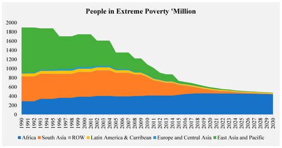
Figure 1.
Poverty in Sub-Saharan Africa. Source: World Bank (2019).
However, the theoretical underpinnings of the FDI–poverty nexus are far from being conclusive. For example, advocates of FDI (Mankiw et al. 1992; Hansen and Rand 2006), Soumare (2015); Bharadwaj (2014); Fowowe and Shuaibu (2014) take the view that FDI is welfare-enhancing/reduces poverty. The most obvious link through which FDI affects poverty is through job creation in the host countries (Gohou and Soumare 2012). Beyond that, FDI also delivers a much-warranted transfer of valuable technology and know-how (Javorcik 2015). This positive view of FDI is not universally shared among important scholars in this field (Arabyat 2017; Rye 2016; Gohou and Soumare 2012). One of the most forceful non-proponents of this view is Stiglitz (2002), who argues that FDI is likely to be affected by market imperfections and unequal bargaining power that may elevate inequality and impede welfare enhancement strategies.
An emerging strand of literature argues that the extent to which FDI is welfare-enhancing depends very much on initial conditions or certain circumstances in the host country’s ‘quality institutions and a functioning financial system’ (Arogundade et al. (2021), Yeboua (2020), Jude and Levieuge (2017), and Agbloyor et al. (2016), Lehnert et al. (2013) and Cleeve (2012), Fowowe and Shuaibu (2014). What this means is that host countries with relatively good institutions and developed financial systems are likely to experience more welfare-enhancing effect of FDI compared to nations with poor institutions and less-developed financial systems. Reaching a similar conclusion, the theoretical framework of Chenery and Stout (1966) also provides the theoretical foundation for the importance of external capital flows for low-income countries. In an economy characterized by savings or foreign exchange gaps, the model claims that external finance can play a crucial role in boosting domestic resources.
In an IMF paper entitled, “Why Does FDI Go Where it Goes? New Evidence From the Transition Economies”, Campos and Yuko (2003) identify key factors that are crucial in attracting FDI. They write “countries with a large market, low-cost labor, abundant natural resources, and close proximity to the major Western markets would attract large amounts of FDI inflows. FDI would thus go to countries with favourable initial conditions.”
Derived from these theoretical augments, the broad hypotheses of our study are that (1) neighboring countries’ FDIs have a significant positive impact on the incidence and intensity of a host country’s poverty; (2) improved institutional quality in neighboring countries has a significant impact on the FDI–poverty reduction nexus of a host country.
The non-uniformity of the theoretical arguments highlights the need for more empirical research to further verify if FDI is welfare-enhancing or not. In fact, a brief review of empirical studies on the FDI–poverty nexus proved to be rather ambiguous. While some studies suggest that FDI has a positive impact on poverty reduction (Sukhadolets et al. 2021; Sikandar et al. 2021; Magombeyi and Odhiambo 2018; Ganić 2019), others suggest the opposite: a negative impact (Ali et al. 2009). For example, Sukhadolets et al. (2021) studied the relationship between GDP, FDI, investment in construction, and poverty. The authors compared a number of countries such as the Russian Federation, including a sample of developed and developing nations. Using non-linear autoregressive distributed lag, the study found that investment in construction stimulates the economies of countries in the long term and maintains or reduces the poverty level by increasing the assets of the population.
Using pool mean group estimation techniques, Sikandar et al. (2021) investigated the impacts of six types of foreign capital inflows on the parameters of poverty reduction and agriculture development in the short-term and long-term perspectives across fourteen developing economies of Latin America, Asia, and Eastern Europe. The study found evidence to suggest that poverty reduction could be positively affected by an increase in the values of agricultural exports, foreign direct investment, foreign development assistance, and remittances received from migrant workers. In sharp contrast, using the autoregressive distributed lag (ARDL) model, Ali et al. (2009) found that FDI increased poverty in Pakistan both in the long-run and short-run. The reason for the conflicting results on the impact of FDI on poverty is that majority of these studies neglect the importance of space in their model. Ignoring the importance of spatial interdependence in regional empirical studies may result in either inefficient or biased estimates (Anselin 2009).
While the application of spatial econometrics to FDI literature is still at the embryonic stage, some empirical studies have taken into account the role of third-country effects: Gutiérrez-Portilla et al. (2019) for Spain; Do et al. (2021) for Vietnam; Madariaga and Poncet (2007) for China; Uttama (2015) for Southeast Asia. These studies conclude that FDI in neighboring countries significantly influences the host country’s economy. To the best of this authors’ knowledge, this study is not aware of any literature that has specifically examined the spatial impact of FDI on poverty in Africa. The closest attempt is that of Chih et al. (2021). However, this study failed to account for the role of neighboring countries’ institutional quality on the nexus between FDI and the economy. The study also assumes that what is good for economic growth is also good for the poor. Since economic growth does not imply a reduction in poverty, it is essential we examine: (1) whether neighboring countries’ FDI matters on poverty reduction of the host country, (2) examine the spatial impact of institutional quality on the FDI–poverty nexus in Africa, and (3) determine whether there is a spatial spillover of poverty in Africa.
Doing this study for Africa is vital for the following reasons: (1) the region is challenged with poor welfare, and often termed the world capital of poverty. (2) The positive spillover of FDI in the region may be hampered by a poor institutional environment. As a result, attracting multinational corporations to invest in these conditions may not produce the desired benefits, as investment flourishes in a competitive atmosphere. (3) Since countries in this region belong to a regional organization designed to encourage mutual economic development among member countries, the level of economic activity in one member state may influence economic activity of another country.
The empirical findings from the spatial Durbin model indicate a significant spatial spillover of FDI on the incidence and intensity of poverty in Africa. The results further provide support for the significant role of institutional quality on the nexus between FDI and poverty reduction. Furthermore, the marginal effect results suggest that countries in Africa are not in isolation, i.e., the level of poverty in a particular country is influenced by its determinants in the neighboring country. This calls for a coordinated policy toward eradicating poverty and establishing institutional reform. The rest of this paper is structured as follows: Section 2 provides stylized facts on FDI and the spatial pattern of poverty in Africa. Section 3 houses the methodology and estimation techniques. The presentation and discussion of the empirical results is discussed in Section 4, while Section 5 concludes and provides critical policy implications.
2. African Poverty in Space
This section provides key stylized facts that motivate this study. Figure 2 presents the contour map of headcount poverty across the 47 selected African countries. The map displays spatial clustering of poverty in 1996 and 2019. As shown in the map, there is evidence of higher clustering of poverty in 2019 compared to 1996.
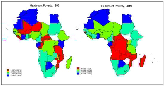
Figure 2.
Spatial pattern of poverty in Africa. Source: Authors’ calculation using data from the World Bank database.
The plots also show that countries such as the Democratic Republic of Congo, Central Africa Republic, Congo Republic, Angola, Zambia, Malawi, Mozambique, Rwanda, Burundi, and Madagascar are epicenters of poverty incidence in Africa in 2019, while countries such as Botswana, Gabon, Ghana, Mauritania, Algeria, Morocco, Tunisia, and Egypt have low poverty rates. In determining whether the incidence of poverty in one country influences the poverty incidence of other proximate countries, this study conducted local and global spatial autocorrelation tests. The former test, which is based on a specific Moran’s I statistic, identifies local “hot spots,” or in other words, the countries where strong spatial correlations exist. The latter test is based on the Moran’s (1950) I spatial autocorrelation statistic; this test determines whether poverty incidence globally observed depends on geographical distribution.
The null hypotheses of these tests suggest that poverty incidence in different countries is considered to be spatially independent. The p-value of the global autocorrelation test is significant, indicating the existence of spatial dependence (see Appendix A Table A1). Similarly, the local indicators of spatial association (LISA) test identifies countries with strong spatial correlations in poverty incidence (see Appendix A Table A2 for more). In addition to this, Figure 3 presents the univariate Global Moran’s I statistic calculated from headcount poverty over the period of 1996 to 2019 for each country.
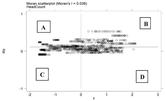
Figure 3.
Global Moran’s I spatial autocorrelation statistic. Source: Author’s computation using data from the World Bank database. Quadrant A in Figure 3 are countries with negative spatial clustering of low poverty incidence, while B indicates countries with positive spatial clustering of high poverty incidence, C indicates positive spatial cluster of countries with low poverty incidence, and D is a negative spatial cluster of high poverty incidence.
The Moran’s I correlation test, which indicates the degree of spatial autocorrelation, suggests a positive spatial clustering of poverty incidence.2 Thus, we can conclude that there is spatial dependence of poverty incidence across African countries from 1996 to 2019. This evidence provides an impetus for the inclusion of space in this study.
Figure 4 shows a scatter plot of FDI and the incidence of poverty in Africa. The plot reveals that countries with relatively high FDI inflows are characterized with high incidence of poverty. However, countries with low FDI inflows are associated with low poverty rate. This indicates that the level of a countries’ foreign investment is positively correlated with the poverty rate. This is also consistent with the argument of Rye (2016) and Arabyat (2017), who argue that foreign investment increases poverty due to its crowd-out effect on domestic capital. This conjecture is perhaps meaningless and lacks objectivity if not subjected to empirical verification.
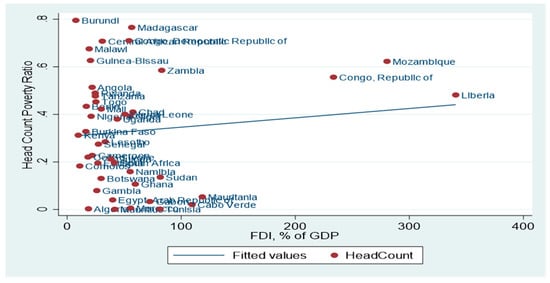
Figure 4.
Scatter plot of FDI and poverty in Africa. Source: Authors’ computation from World Bank PovcalNet and UNCTAD database.
The scatter plot of the institution quality1 and poverty rate is presented in Figure 5. The figure reveals that countries with relatively high poverty incidence are characterized by poor institutional frameworks. However, countries with a robust institutional framework have relatively low poverty rate. Countries with sound institutions, such as efficient and good governance, low corruption, rule of law, and property rights, tend to improve the process of technology spillovers to local enterprises. On the other hand, countries with weak institutions may prevent indigenous enterprises from benefiting from multinational corporation (MNC) knowledge and technology spillovers (Agbloyor et al. 2016; Brahim and Rachidi 2014). Hence, the impact of FDI on poverty reduction is expected to vary between countries and regions with varying level of institutional quality.
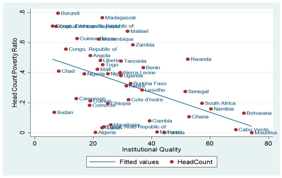
Figure 5.
Scatter plot of institutional quality and poverty in Africa. Source: Author’s computation based on World Governance Indicator and World Bank Povcal Database (World Bank 2019).
3. Data and Methodology
3.1. Data
This study employs a panel dataset of 44 African countries, with annual data over the period of 1996–2019. The choice of period and countries (see Appendix A Table A1) were dictated by the availability of data. In this study’s analysis, we follow Gnangnon (2020), Agarwal et al. (2017), and Perera and Lee (2015) by using headcount ratio, which is a measure of the incidence of poverty and poverty gap index, which measures the intensity of poverty. Both headcount and poverty gap indexes are measured using the international poverty line of $1.90 per day. This study follows Arogundade et al. (2022) and Nunnenkamp (2004) by measuring FDI as FDI inward stock as a percentage of GDP. The problem of endogeneity biases linked with the FDI–welfare nexus is also mitigated by using FDI stock (Nunnenkamp 2004). We used the International Monetary Fund’s newly constructed aggregate financial development index to measure financial development. Other metrics such as credit to the private sector, stock market capitalization, and monetary aggregates have flaws as they do not capture the financial system’s multidimensionality, which is why this index was created. See Arogundade et al. (2021) for a similar approach. Institutional quality is measured using the average of the six indicators (voice and accountability, the rule of law, regulatory quality, control of corruption, government effectiveness, and political stability). These indexes range from 0 (weak) to 100 (strong). See Siriopoulos et al. (2021), Peres et al. (2018), Utesch-Xiong and Kambhampati (2021), and Ajide and Raheem (2016) for a similar approach. In measuring infrastructure, we used mobile telephone subscribers (per 100 people). We use the growth rate of GDP per capita as a proxy for economic growth and the total active labor force as a proxy for labor, as Kaulihowa (2017) suggests.
Descriptive Statistics of the Variables
Table 1 shows the descriptive statistics of the variables used in this study. From 1996 to 2019, and among the 44 countries, the average values for poverty headcount and poverty gap were 41.6 percent and 17.4 percent for poverty headcount and poverty gap, respectively. Ghana has the minimum level of headcount and poverty gap rate, with 0.13% and 0.015% respectively of its population. However, the Congo Democratic Republic has the highest headcount and poverty gap at 95.3 and 66.5%, respectively. For FDI inward stock, the average is 39.23%, with a minimum of 0.224 and a maximum of 1039 %. Institutional quality ranged from 77.40 to 1.182, with an average of 31.87. Congo Democratic Republic has the lowest institutional score, while Mauritius has the highest. The pairwise correlation measures the relative association among the dependent variables and regressors. The results indicate that except for labor (L), all the variables have statistically significant relationships with the poverty rate. However, the signs vary. A cursory look at Table 2 also indicates that all correlation statistics are below 0.80. Hence, no evidence of multicollinearity among the covariates.

Table 1.
Summary Statistics.
Table 2.
Pairwise Correlation.
3.2. Methodology
This study follows other spatial studies like Uttama (2015), Do et al. (2021), and Chih et al. (2021) by initially using a simple regression model as the benchmark model. The Driscoll and Kraay (1998) robust-standard-errors-type approach, which accounts for heteroskedasticity, autocorrelation, and cross-sectional dependence is used in this study. This is nested into the fixed effect instrumental variable regression model (FE-2SLS). The choice of the instrument (lagged FDI) used in this study is based on the instrument relevance and exogeneity conditions. The empirical form of the model without spatial interaction is given as follows:
where is poverty rate in country at period; is FDI inward stock as a percentage of GDP in country at period ; is the vector control variables which includes GDP growth, labor, institutional quality, financial development, and infrastructure; is country-specific effect that is time-invariant; and is the error term. Equation (1.0) is the first stage of the FE-2SLS model, while Equation (2) is the second stage. This study uses the probability value of the F-test in equation (1.0) as instrument relevance test. in Equation (2) is the interaction term of FDI with institutional quality. We included both and institutional quality in Equation (2) to ensure that the interaction term does not proxy for either or the . If and , it suggests that FDI reduces poverty at high level of institutional quality. For robustness of our empirical estimate, we used the instrumental variables techniques nested within the generalized method of moments (IV-GMM) framework by Baum et al. (2007a, 2007b).
Since the estimate of Equation (2) is inconsistent and biased due to the possibility of spatial interdependence that exists in the independent(s) or dependent variable (Anselin 2009), we augment Equation (2) with spatial characteristics as shown in Equations (3) and (4). Spatial interdependence can be introduced into a simple regression model in three ways: as an additional covariate referred to as spatial autoregressive (SAR) () or spatial Durbin model (SDM) ( or through the error structure known as the spatial error model (SEM) . The Wald and likelihood ratio test is used to determine the choice of the spatial autoregressive models, since the models are estimated using maximum likelihood (Anselin 1988; Anselin and Bera 1998). We follow LeSage and Pace (2009) by using two different hypotheses. The first is . This hypothesis examines whether Equations (3) and (4) can be reduced to a SAR model. The second hypothesis is , which suggests whether Equations (3) and (4) can be reduced to a SEM model. We further use the likelihood ratio (LR), which was initially proposed by Burridge (1980) to determine between the SAR and SDM model. According to Hao et al. (2020), if both the Wald and LR test are rejected, this suggest that the best model for the data is SDM.
where
where is a non-negative matrix describing the spatial arrangement or configuration of the units in the sample. Parameter in Equation (3) measured the impact of the neighboring countries’ poverty on host country poverty. is the elasticity of neighboring countries FDI on the host country poverty. is the mediating impact of neighboring countries’ institutional quality on FDI–poverty nexus. is spatial error parameter, and interaction effects among the disturbance term of the different spatial units, ε is a stochastic disturbance with . According to Anselin and Gallo (2006), one of the major problems of fixed effect spatial lag model is the possibility of endogeneity of the spatial lag which violates the assumption of standard regression models . In addressing this simultaneity bias, this study uses the maximum likelihood estimation3.
3.2.1. Direct, Indirect, and Total Effects
Interpretation of models containing spatial lags of the dependents or explanatory variables becomes more complicated and richer. However, several research have claimed that models with spatial lag in the dependent variable necessitate a different interpretation of the parameters. These studies further posit that utilizing point estimation methods to analyze spatial spillover effects might lead to incorrect findings, and that partial differential approaches can explain the impacts of variable changes in the model. (LeSage and Pace 2009; Anselin and Gallo 2006; Kelejian et al. 2006). The specification of the spatial spillover effect is specified thus as:
The direct effect should be quantified using the arithmetic mean of the elements on the matrix’s main diagonal, while the indirect effect should be measured using the mean value of the elements on the non-diagonal line (LeSage and Pace 2009).
3.2.2. Spatial Weight Matrix
The spatial weight matrix signifies the strength of the interaction or similarity between spatial units, i.e., country and . This study specifies two proximity weight matrices for the spatial model. This includes contiguity and inverse distance. In creating the spatial weight matrix , we follow other spatial studies by normalizing the matrix such that each row sums to unity. The weighting matrix for contiguity is defined as:
This study employs the inverse-distance spatial weighting matrix as an alternative measure of spatial weight matrix. The inverse distance is made up of weights that are inversely proportional to the unit distances. This is specified thus as:
explains the functional form of the weights between any two host nations and . The spatial weighting matrix for the inverse distance is a block diagonal, with each block representing a single year of observation. For any year, , is defined as:
is the distance between host and . The diagonal elements of are set to zero since no spatial unit can be its own neighbor. This approach allows all countries to affect each other.
3.2.3. Spatial Autocorrelation Test
The main variable should be investigated to discover the spatial dependence before using the spatial econometric model. Moran’s I is a technique for determining whether a variable is spatially dependent. The following is the formula:
The Moran’s I value ranges between −1 and 1; a negative Moran’s I denotes a negative correlation, while a positive value indicates a positive spatial correlation.
4. Empirical Results and Discussion
4.1. Baseline Results
The baseline results on the direct impact of FDI on poverty in Africa is presented in Table 3. The coefficient of financial development indicates that financial development has a positive and significant impact on the incidence and intensity of poverty. This finding aligns with Rewilak (2017)’s empirical outcome, which argues that financial development increases the incidence of poverty. However, the result of the IV-GMM suggests that financial development has a negative and statistical impact on the incidence and intensity of poverty. This aligns with the findings of Donou-Adonsou and Sylwester (2016) and Jalilian and Kirkpatrick (2019), who argue that an economy characterized by a developed financial system can mobilize savings for investment, and as such, reduce poverty. The significance and positive sign of infrastructure across models indicate that infrastructure availability is vital to Africa’s poverty reduction. Studies such as Seetanah et al. (2009) and Anyanwu and Erhijakpor (2009) reached a similar conclusion.
Table 3.
Baseline Results: Non-Spatial Model.
Furthermore, the impact of labor on poverty is mixed, while the negative and significant coefficient in the FE-2SLS model is in tandem with Colen et al. (2009)’s argument that a rising active labor force reduces unemployment rate and poverty. The positive impact of coefficients of active in the IV-GMM model indicates that a growing labor force can increase the number of poor people and their intensity. This is conceivable since Africa’s labor force is largely made up of young people, with a high proportion of them unemployed. Poverty reduction is also influenced by the rate of economic growth; as claimed by the estimates, growth in GDP per capita has a negative and statistically significant impact on poverty in Africa. This is in line with the findings of Son and Kakwani (2004), who claim that increasing economic activity through aggregate demand, factor productivity lower unemployment rates and poverty alleviation.
Additionally, the impact of institutional quality on poverty is also mixed. The results of the FE-2SLS model indicates that institutional quality has a negative and significant relationship with poverty. This demonstrates that countries with strong institutional quality systems may boost economic growth, reduce income inequality, and reduce poverty. This is consistent with the study of (Sobhee 2017; Perera and Lee 2015. However, estimates from the IV-GMM indicates that institutional quality increases poverty, which is at odds with empirical literature.) The impact of FDI on the incidence and intensity of poverty is positively significant, indicating that FDI exacerbates poverty situations of African countries. This finding is in line with Arabyat (2017), Rye (2016), and Gohou and Soumare (2012), who attribute profit repatriation by multinational companies, the crowding-out effect of foreign investment on domestic capital, and a low level of host absorptive capacity as factors causing FDI to exacerbate poverty in the region.
The interaction of FDI and institutional quality reveals a negative and statistically significant impact on the poverty measures. This suggests that an increase in institution quality has a favorable and significant impact on the FDI–poverty reduction nexus in Africa. This finding is consistent with the findings of Hayat (2019), Jilenga and Helian (2017), and Agbloyor et al. (2016), who found that countries with high institutional quality have the potential to reap the benefits of FDI through healthy competition, improved spillovers, and capital accumulation.
4.2. Spatial Pre-Estimation Test
In this section, we examine whether spatial dependence exists in the model specified in Equation (2). This test is based on the residuals of the non-spatial results of the pooled regression, which is not reported in this study but available on request. The Moran’s I test results shown in Table 4, indicates a rejection of the null hypothesis of no spatial interdependence. In addition to this, the results of the Lagrange Multiplier and Robust Lagrange Multiplier (RLM) suggest rejection of the null hypothesis of no spatial lag as against the alternative hypothesis of spatial error and spatial lag dependence. Following the general-to-specific approach, the SDM is the appropriate specification if the spatial error effect and spatial lag are detected. The Geary C test also demonstrate the existence of global spatial autocorrelation as the null hypothesis that “there is no global spatial autocorrelation is rejected. The validity of the SDM should be confirmed with the Wald test and likelihood ratio (Do et al. 2021; Ragoubi and El Harbi 2018).
Table 4.
Spatial Pre-estimation test.
4.3. Spatial Impact of FDI on Poverty in Africa—Contiguity
As shown in Table 5, we can infer that the best model that best describes our data is the spatial durbin model (SDM), since the null hypothesis of the Wald and LR test are rejected. Furthermore, the Hausman test has confirmed the suitability of the SDM-FE model. Using the baseline proximity matrix specified in Equation (6), the coefficient of the spatial lag of FDI is significant and positive suggesting that ignoring spatial dependence in the model would have resulted in biased estimates. The statistical significance of the weighted FDI suggests significant spillover of neighboring countries FDI on host country poverty condition. Furthermore, the intuition of this empirical outcome is that the activity of multinational corporation in proximate countries deteriorate welfare conditions of host country. The channel of the impact could be through the crowd-out effect and profit repatriation. Similarly, the weighted coefficient of FDI interacted with institutional quality is statistically significant and negative, indicating that neighboring countries institutional quality matters in the nexus between FDI and poverty. This call for a mutual corporation in building a robust institutional quality before African countries can reap the benefit of FDI. Our empirical results further indicate spatial spillover of incidence and intensity of poverty in the region, since the coefficient of the spatial poverty is positive. The intuition behind this positive impact is African migrants migrate to other neighboring countries to seek greener pastures. This then has implication on the poverty conditions of the host country.
Table 5.
Spatial impact of FDI on Poverty in Africa (Spatial Weight: Contiguity).
4.4. Marginal Effect Estimation Results
This section presents the direct, indirect, total, and feedback impacts of FDI on poverty in Africa. The headcount ratio is employed as a poverty measure since the goal of development specialists is to minimize the overall number of poor people (the results of the poverty gap are not reported due to brevity but available on request). The direct impact demonstrates that the change in the region-dependent variable (poverty) is because of the explanatory variables (FDI, financial development, infrastructure, labor, institutional quality, economic growth, and FDI*inst) of the same region. Whereas, the indirect (spillover) effects capture the change in the endogenous variable that is caused by the independent variables of other regions (neighboring countries). The total impact is the sum of direct and indirect effects. Table 5 presents the estimated marginal effect using the SDM-FE model. These estimates are vital to governments of African countries since it gives them a comprehensive knowledge of how their poverty conditions could be influenced by neighboring countries’ FDI and other poverty determinants. The direct results suggest that a one percent increase in FDI and financial development in country increases the incidence of poverty of country by 0.013% and 2.917%, respectively. However, the impact of infrastructure, labor, institutional quality, economic growth, and the interaction of institutional quality with FDI reduces poverty by 0.057%, 18.23, 0.101%, 0.162%, and 0.001%, respectively.
The indirect estimates/spillover effect provided in column 2 suggest spillover effect in the region. The results show that a one percent increase in FDI and financial development in country has a positive spillover effect of 0.057% and 0.270%, 0.270% on the poverty rate of country . However, the impact of other variables like infrastructure, labor, institutional quality, economic growth, and the interaction of institutional quality with FDI reduces poverty rate by 0.01%, 1.69%, 0.01%, 0.015%, 0.015%, respectively. Since most of the coefficients of the indirect effect are significant, we can conclude that policies geared toward poverty reduction in African countries should not be treated in isolation, as there is evidence of both direct and spillover effects of poverty determinants in Africa, i.e., the poverty condition of a particular country is influenced by the poverty conditions of other neighboring countries and its determinant.
4.5. Spatial Impact of FDI on Poverty in Africa—Distance
This study uses the inverse distance (specified in equation 8) as the alternative measure of proximity for our empirical estimation. The results presented in Appendix A Table A3 are in similitude with that of Table 5. The only difference is that all the weighted poverty rates are negative for both incidence and intensity of poverty (. The control variables also generally have the expected signs and are statistically significant. The results of the cumulative marginal effect of the distance proximity matrix are also in similitude with the contiguity results presented in Table 6. However, the results are not reported in this study due to brevity, although they are available upon request.
Table 6.
Marginal effect estimation results.
5. Discussion
In the study we focus more on the role of space in the impact of FDI on poverty in Africa. We further compare our results with the existing studies in the literature that failed to take into account the role of space. Evidence from the SAR regression indicates that a percentage increase in poverty in country ‘i’ increases the country’s ‘j’ poverty rate by 0.12%. This implies that there is interdependence of poverty among African countries. Furthermore, a significant spatial dependence was also observed in the SDM model. This result is consistent with the empirical outcome of Qin and Zhang (2022) and Ullah et al. (2020) that there is a significant spatial spillover of poverty.
Additionally, we found that neighboring countries’ FDIs have a positive and significant impact on the incidence and intensity of a host country’s poverty. This implies that not controlling for spatial dependence may trigger biased results. Studies such as Uttama (2015) and Chih et al. (2021) found similar results for Asia and Africa, respectively. Their argument is that proximate country FDIs influence the economic performance of a host country.
Further empirical results from the SDM model indicates that neighboring countries’ institutional quality play a significant role in the nexus between FDI and poverty reduction in Africa. This aligns with the empirical outcome in Arogundade et al. (2021) that governance mediates the positive impact of FDI on poverty reduction in Africa. This highlights the importance of institutional reforms in Africa, as investments do not thrive in an environment characterized by weak institutional quality.
6. Conclusions and Recommendations
In reducing the savings gap and achieving equitable and sustainable development, a large amount of quality foreign resources is required in Africa. Hence, foreign investments, such as FDI, are seen as one of the most important drivers of economic development in the region by policymakers. However, empirical studies examining the impact of FDI on poverty have reached varying results. While some studies argue that FDI reduces poverty, some studies believe that it increases poverty. Other studies posit that FDI’s impact is conditional on certain intermittent variables. The reason for the diverse findings on the impact of FDI is that the majority of these studies neglect the role of space. In contributing to the literature, this study assesses whether spatial interdependence/third-country effects matter in the impact of FDI on the incidence and intensity of poverty in Africa. In achieving this, the study employed the spatial Durbin model to quantify the impact of neighboring country FDIs on the poverty conditions of a host country. Before accounting for space in our model, the study conducted some pre-estimation tests to determine the existence of spatial spillover on the effect of FDI. The results indicate that neighboring country FDIs impact a host country’s poverty. Hence, neglecting spatial interdependence in the FDI model may result to biased estimates.
This study’s empirical findings are as follows: (1) neighboring country FDIs have a significant and positive impact on the incidence and intensity of the host country, (2) neighboring countries’ institutional quality matters in the nexus between FDI and poverty reduction, since the positive impact of FDI on poverty is mitigated through a robust institutional quality, (3) there is a significant spatial spillover of neighboring countries’ poverty to a host country, (4) the marginal effect results indicate that countries within the region are no longer in isolation or independent; i.e., the level of poverty in a particular country is influenced by its determinants in the neighboring country. This result is robust to the different proximity matrix, which is the inverse distance.
The empirical results of this study have produced important policy implications for African governments. First, since FDI does not reduce poverty from our empirical estimation, African countries need to embark on public sector reforms, as investment would not thrive when there is high corruption, low voice and accountability, government inefficiency, poor regulatory quality, low rule of law, and political instability. Second, since the empirical results of this study provide evidence of both direct and spillover effects of poverty determinants, we recommend that African countries consider their surrounding countries’ characteristics in their welfare policy formulation. The study also highlights the importance of joint task efforts toward building strong institutional quality. This is to permit African countries to have coordinated policies towards building a robust institutional framework. African governments through the African Union (AU) or other relevant agencies are encouraged to not only develop an institutional reform for Africa, but also establish a binding mechanism to ensure reform implementation.
7. Future Research
This study has some shortcomings which can be addressed in future research. Other intermittent or mediating variables such as financial development, globalization, and International Financial Reporting Standards (IFRS) have all been shown to be crucial. Future research could investigate the impact of these variables on the nexus between FDI and poverty within spatial framework. Future studies could also extend the topic to other continents using spatial models. Moreover, this study only uses the income measure of poverty. Future studies are encouraged to consider other non-income poverty measures.
Author Contributions
Conceptualized the major idea of this research paper, Prepared the methodology, data collection, analysis, interpretation, and conclusion section, S.A.; Prepared the literature review and general editing, M.B.; Prepared the introduction and formatting, S.B. All authors have read and agreed to the published version of the manuscript.
Funding
This research received no external funding.
Institutional Review Board Statement
Not applicable.
Informed Consent Statement
Not applicable.
Data Availability Statement
The datasets used and/or analyzed during the current study are available from the author on reasonable request.
Conflicts of Interest
The authors declare no conflict of interest.
Appendix A
Table A1.
Moran’s Residual of Headcount Poverty Regression by Country *.
Table A1.
Moran’s Residual of Headcount Poverty Regression by Country *.
| Countries | * | |||
|---|---|---|---|---|
| Algeria | 0.133 | 0.018 | 7.255 | 0.000 |
| Angola | 0.054 | 0.016 | 3.396 | 0.001 |
| Benin | 0.006 | 0.040 | 0.162 | 0.871 |
| Botswana | −0.133 | 0.025 | −5.351 | 0.000 |
| Burkina Faso | −0.005 | 0.028 | −0.130 | 0.896 |
| Burundi | 0.625 | 0.050 | 12.403 | 0.000 |
| Cabo Verde | −0.067 | 0.024 | −2.733 | 0.006 |
| Cameroon | −0.088 | 0.020 | −4.317 | 0.000 |
| Central African Republic | 0.103 | 0.017 | 6.180 | 0.000 |
| Chad | −0.001 | 0.016 | −0.019 | 0.985 |
| Comoros | −0.276 | 0.023 | −12.220 | 0.000 |
| DRC | 0.237 | 0.020 | 11.705 | 0.000 |
| Republic of Congo | 0.008 | 0.025 | 0.359 | 0.720 |
| Cote d’Ivoire | −0.092 | 0.029 | −3.126 | 0.002 |
| Egypt | −0.045 | 0.015 | −2.997 | 0.003 |
| Ethiopia | −0.104 | 0.019 | −5.409 | 0.000 |
| Gabon | −0.274 | 0.026 | −10.664 | 0.000 |
| Gambia | −0.183 | 0.061 | −2.985 | 0.003 |
| Ghana | −0.186 | 0.036 | −5.133 | 0.000 |
| Guinea | −0.121 | 0.040 | −3.036 | 0.002 |
| Guinea-Bissau | −0.019 | 0.052 | −0.345 | 0.730 |
| Kenya | −0.107 | 0.025 | −4.288 | 0.000 |
| Lesotho | 0.023 | 0.039 | 0.607 | 0.544 |
| Liberia | 0.013 | 0.033 | 0.422 | 0.673 |
| Madagascar | 0.022 | 0.023 | 1.017 | 0.309 |
| Malawi | 0.277 | 0.028 | 9.999 | 0.000 |
| Mali | −0.001 | 0.023 | −0.007 | 0.994 |
| Mauritania | −0.025 | 0.023 | −1.030 | 0.303 |
| Mauritius | −0.393 | 0.023 | −17.297 | 0.000 |
| Morocco | 0.147 | 0.019 | 7.734 | 0.000 |
| Mozambique | 0.170 | 0.028 | 6.130 | 0.000 |
| Namibia | −0.060 | 0.022 | −2.729 | 0.006 |
| Niger | 0.002 | 0.017 | 0.154 | 0.878 |
| Nigeria | −0.005 | 0.021 | −0.178 | 0.859 |
| Rwanda | 0.154 | 0.051 | 3.066 | 0.002 |
| Senegal | −0.021 | 0.057 | −0.349 | 0.727 |
| Sierra Leone | −0.005 | 0.041 | −0.106 | 0.916 |
| South Africa | −0.072 | 0.039 | −1.839 | 0.066 |
| Sudan | −0.090 | 0.016 | −5.675 | 0.000 |
| Tanzania | 0.071 | 0.025 | 2.864 | 0.004 |
| Togo | 0.003 | 0.043 | 0.095 | 0.925 |
| Tunisia | 0.156 | 0.017 | 9.286 | 0.000 |
| Uganda | −0.045 | 0.028 | −1.555 | 0.120 |
| Zambia | 0.157 | 0.021 | 7.418 | 0.000 |
| Measures of global spatial autocorrelation | ||||
| 0.927 | 0.003 | −21.681 | 0.000 | |
* The probability level is two-tail test. NB: the LISA test of countries in the sample is estimated using year 2019, which is the end of our study period.
Table A2.
United Nation Regional Classification.
Table A2.
United Nation Regional Classification.
| Algeria | Comoros | Guinea | Morocco | Sudan |
|---|---|---|---|---|
| Angola | Congo, Democratic Republic of | Guinea-Bissau | Mozambique | Tanzania |
| Benin | Congo, Republic of | Kenya | Namibia | Togo |
| Botswana | Cote d’Ivoire | Lesotho | Niger | Tunisia |
| Burkina Faso | Djibouti | Liberia | Nigeria | Uganda |
| Burundi | Egypt | Madagascar | Rwanda | Zambia |
| Cabo Verde | Ethiopia | Malawi | Senegal | Zimbabwe |
| Cameroon | Gabon | Mali | Seychelles | |
| Central African Republic | Gambia | Mauritania | Sierra Leone | |
| Chad | Ghana | Mauritius | South Africa |
Table A3.
Spatial impact of FDI on Poverty in Africa (Spatial Weight: Distance).
Table A3.
Spatial impact of FDI on Poverty in Africa (Spatial Weight: Distance).
| (1) | (2) | (3) | (4) | (5) | (6) | |
|---|---|---|---|---|---|---|
| VARIABLES | SAR Model | SDM Model | SEM Model | |||
| Headcount | Poverty Gap | Headcount | Poverty Gap | Headcount | Poverty Gap | |
| FDI | 0.0001 | 5.47 × 10⁻⁵ | 0.0001 | 7.11 × 10⁻⁵ | 0.0002 ** | 0.0001 ** |
| (7.78 × 10⁻⁵) | (5.79 × 10⁻⁵) | (7.72 × 10⁻⁵) | (5.70 × 10⁻⁵) | (7.85 × 10⁻⁵) | (5.92 × 10⁻⁵) | |
| Financial Devt. | 0.0881 | 0.159 ** | 0.0473 | 0.105 | 0.115 | 0.155 ** |
| (0.0920) | (0.0684) | (0.0919) | (0.0680) | (0.0893) | (0.0657) | |
| Infrastructure | −0.0007 *** | −0.0003 *** | −0.00071 *** | −0.0002* | −0.0008 *** | −0.0003 *** |
| (0.0001) | (9.16 × 10 -5) | (0.0001) | (9.61 × 10 -5) | (0.0001) | (7.10 × 10 -5) | |
| Labor | −0.206 *** | −0.149 *** | −0.232 *** | −0.163 *** | −0.184 *** | −0.156 *** |
| (0.0281) | (0.0210) | (0.0309) | (0.0237) | (0.0179) | (0.0128) | |
| Inst | −0.0014 *** | −0.0016 *** | −0.0013 *** | −0.0016 *** | −0.0014 *** | −0.0017 *** |
| (0.0005) | (0.0004) | (0.0005) | (0.0003) | (0.0005) | (0.0003) | |
| Economic Growth | −0.0018 *** | −0.0013 *** | −0.0017 *** | −0.0012 *** | −0.0021 *** | −0.0016 *** |
| (0.0006) | (0.0004) | (0.0006) | (0.0004) | (0.0006) | (0.0004) | |
| −4.62 × 10⁻⁶ | −3.31 × 10⁻⁶ | −4.94 × 10⁻⁶* | −3.93 × 10⁻⁶ * | −4.62 × 10⁻⁶ | −3.54 × 10⁻⁶ | |
| (3.01 × 10⁻⁶) | (2.24 × 10⁻⁶) | (2.99 × 10⁻⁶) | (2.21 × 10⁻⁶) | (2.96 × 10⁻⁶) | (2.19 × 10⁻⁶) | |
| 0.0017 *** | 0.00162 *** | |||||
| (0.0004) | (0.0003) | |||||
| −3.84 × 10⁻⁵ ** | −5.99 × 10⁻⁵ *** | |||||
| (1.80 × 10⁻⁵) | (1.33 × 10⁻⁵) | |||||
| −0.0548 | 0.0148 | −0.153 | −0.221 ** | |||
| (0.0931) | (0.0983) | (0.101) | (0.111) | |||
| ) | −0.597 *** | −0.684 *** | ||||
| (0.145) | (0.154) | |||||
| Number of Countries | 44 | 44 | 44 | 44 | 44 | 44 |
| Prob > χ2 a | 721.63 *** | 525.77 *** | 753.55 *** | 525.77 *** | 1860.49 *** | 1356.69 *** |
| SEM vs. SDM b | 4.26 *** | 5.36 *** | ||||
| (0.0004) | (0.0003) | |||||
| SAR vs. SDM (LR test) c | 18.12 *** | 32.78 *** | ||||
Standard errors in parentheses, *** denotes significance at 1%, ** at 5%, and * at 10%. The Hausman test suggests fixed effect over random effect model; the report is available on request. All regressions are estimated using maximum-likelihood estimator. a: Joint significance of all the variables. b: Wald test of spatial terms. c: Log likelihood ratio test.
Notes
| 1 | As measured by the average of the six dimensions of institutional quality in 2019. |
| 2 | As measured by head count poverty as a percentage of population in 2019. |
| 3 | See Elhorst (2014) for more on the mathematical derivation. |
References
- Agarwal, Manmohan, Pragya Atri, and Srikanta Kundu. 2017. Foreign direct investment and poverty reduction: India in regional context. South Asia Economic Journal 18: 135–57. [Google Scholar] [CrossRef]
- Agbloyor, Elikplimi Komla, Agyapomaa Gyeke-Dako, Ransome Kuipo, and Joshua Yindenaba Abor. 2016. Foreign direct investment and economic growth in SSA: The role of institutions. Thunderbird International Business Review 58: 479–97. [Google Scholar] [CrossRef]
- Ajide, K. Bello, and Ibrahim Dolapo Raheem. 2016. Institutions-FDI nexus in ECOWAS countries. Journal of African Business 17: 319–41. [Google Scholar] [CrossRef]
- Ali, Muhammad, Muhammad Nishat, and Talat Anwar. 2009. Do foreign inflows benefit Pakistani poor? [with comments]. The Pakistan Development Review 48: 715–38. [Google Scholar] [CrossRef] [Green Version]
- Anselin, Luc. 1988. Lagrange multiplier test diagnostics for spatial dependence and spatial heterogeneity. Geographical Analysis 20: 1–17. [Google Scholar] [CrossRef]
- Anselin, L. 2009. Spatial regression. In The SAGE Handbook of Spatial Analysis. Newcastle upon Tyne: Sage, Volume 1, pp. 255–76. [Google Scholar]
- Anselin, Luc, and Anil K. Bera. 1998. Spatial dependence in linear regression models with an introduction to spatial econometrics. Statistics Textbooks and Monographs 155: 237–90. [Google Scholar]
- Anselin, Luc, and Julie Le Gallo. 2006. Interpolation of air quality measures in hedonic house price models: Spatial aspects. Spatial Economic Analysis 1: 31–52. [Google Scholar] [CrossRef]
- Anyanwu, John C., and Andrew EO Erhijakpor. 2009. The Impact of Road Infrastructure on Poverty Reduction in Africa. New York: Poverty in Africa, Nova Science Publishers, Inc., pp. 1–40. [Google Scholar]
- Arabyat, Yaser. 2017. The Impact of FDI on poverty reduction in the Developing Countries. International Finance and Banking 4. [Google Scholar] [CrossRef]
- Arogundade, Sodiq, Mduduzi Biyase, and Joel H. Eita. 2021. Foreign Direct Investment and Inclusive Human Development in Sub-Saharan African Countries: Domestic Conditions Matter. Economia Internazionale/International Economics 74: 463–98. [Google Scholar]
- Arogundade, Sodiq, Adewale Samuel Hassan, and Santos Bila. 2022. Adewale Samuel Hassan, and Santos Bila. 2022. Diaspora Income, Financial Development and Ecological footprint in Africa. International Journal of Sustainable Development & World Ecology, 1–15. [Google Scholar] [CrossRef]
- Baum, Christopher F., Mark E. Schaffer, and Steven Stillman. 2007a. Enhanced Routines for Instrumental Variables/Generalized Method of Moments Estimation and Testing. Stata Journal 7: 465–506. [Google Scholar] [CrossRef]
- Baum, Christopher F., Mark E. Schaffer, and Steven Stillman. 2007b. ivreg2: Stata Module for Extended Instrumental Variables/2SLS, GMM and AC/HAC, LIML, and k-Class Regression. Boston: Boston College Department of Economics, Statistical Software Components, p. S425401. [Google Scholar]
- Bharadwaj, Ashish. 2014. Reviving the globalization and poverty debate: Effects of real and financial integration on the developing world. Advances in Economics and Business 2: 42–57. [Google Scholar] [CrossRef]
- Brahim, Mariem, and Houssem Rachdi. 2014. Foreign direct investment, institutions and economic growth: Evidence from the MENA region. Journal of Reviews on Global Economics 3: 328–39. [Google Scholar]
- Burridge, Peter. 1980. On the Cliff-Ord test for spatial correlation. Journal of the Royal Statistical Society: Series B (Methodological) 42: 107–8. [Google Scholar] [CrossRef]
- Campos, Nauro, and Kinoshita Yuko. 2003. Why Does FDI Go Where it Goes?: New Evidence from the Transition Economies. IMF Working Paper, WP/03/228. Washington, DC: International Monetary Fund. [Google Scholar]
- Chenery, Hollis, and A. Stout. 1966. Foreign assistance and economic development. American Economic Review 56: 679–733. [Google Scholar]
- Chih, Yao-Yu, Ruby P. Kishan, and Andrew Ojede. 2021. Be good to thy neighbors: A spatial analysis of foreign direct investment and economic growth in sub-Saharan Africa. The World Economy 45: 657–701. [Google Scholar] [CrossRef]
- Cleeve, Emmanuel. 2012. Political and institutional impediments to foreign direct investment inflows to sub-Saharan Africa. Thunderbird International International Business Review 54: 469–77. [Google Scholar] [CrossRef]
- Colen, Liesbeth, Miet Maertens, and Johan Swinnen. 2009. Foreign direct investment as an engine for economic growth and human development: A review of the arguments and empirical evidence. Hum. Rts. & Int’l Legal Discourse 3: 177. [Google Scholar]
- Do, Quynh Anh, Quoc Hoi Le, Thanh Duong Nguyen, Van Anh Vu, Lan Huong Tran, and Cuc Thi Thu Nguyen. 2021. Spatial Impact of Foreign Direct Investment on Poverty Reduction in Vietnam. Journal of Risk and Financial Management 14: 292. [Google Scholar] [CrossRef]
- Donou-Adonsou, Ficawoyi, and Kevin Sylwester. 2016. Financial development and poverty reduction in developing countries: New evidence from banks and microfinance institutions. Review of Development Finance 6: 82–90. [Google Scholar] [CrossRef] [Green Version]
- Driscoll, J. C., and A. C. Kraay. 1998. Consistent covariance matrix estimation with spatially dependent panel data. Review of Economics and Statistics 80: 549–60. [Google Scholar] [CrossRef]
- Elhorst, Paul. 2014. Spatial Econometrics: From Cross-Sectional Data to Spatial Panels. Heidelberg: Springer, vol. 479, p. 480. [Google Scholar]
- Fowowe, B., and M. I. Shuaibu. 2014. Is foreign direct investment good for the poor? New evidence from African countries. Economic Change and Restructuring 47: 321–39. [Google Scholar] [CrossRef]
- Ganić, M. 2019. Does Foreign Direct Investment (FDI) contribute to poverty reduction? Empirical evidence from Central European and Western Balkan Countries. Scientific Annals of Economics and Business 66: 15–27. [Google Scholar] [CrossRef] [Green Version]
- Gnangnon, S. K. 2020. Does Poverty deter Foreign Direct Investment flows to Developing Countries? Preprints. [Google Scholar] [CrossRef]
- Gohou, G., and I. Soumare. 2012. Does foreign direct investment reduce poverty in Africa and are there regional differences? World Development 40: 75–95. [Google Scholar] [CrossRef]
- Gutiérrez-Portilla, P., A. Maza, and J. Villaverde. 2019. A spatial approach to the FDI-growth nexus in Spain: Dealing with the headquarters effect. International Business Review 28: 101597. [Google Scholar] [CrossRef]
- Hansen, H., and J. Rand. 2006. On the causal links between FDI and growth in developing countries. The World Economy 29: 21–41. [Google Scholar] [CrossRef] [Green Version]
- Hao, Y., Y. Wu, H. Wu, and S. Ren. 2020. How do FDI and technical innovation affect environmental quality? Evidence from China. Environmental Science and Pollution Research 27: 7835–50. [Google Scholar] [CrossRef]
- Hayat, A. 2019. Foreign direct investments, institutional quality, and economic growth. The Journal of International Trade & Economic Development 28: 561–79. [Google Scholar]
- Jalilian, H., and C. Kirkpatrick. 2019. Financial development and poverty reduction in developing countries. International Journal of Finance & Economics 7: 97–108. [Google Scholar]
- Javorcik, B. S. 2015. Does FDI bring good jobs to host countries? The World Bank Research Observer 30: 74–94. [Google Scholar] [CrossRef] [Green Version]
- Jilenga, M. T., and X. Helian. 2017. Foreign direct investment and economic growth in Sub-Saharan Africa: The role of institutions. Turkish Economic Review 4: 378–87. [Google Scholar]
- Jude, C., and G. Levieuge. 2017. Growth effect of foreign direct investment in developing economies: The role of institutional quality. The World Economy 40: 715–42. [Google Scholar] [CrossRef]
- Kaulihowa, T. 2017. Foreign Direct Investment and Welfare Dynamics in Africa. Ph.D. thesis, Development Finance, Faculty of Economic and Management Sciences at Stellenbosch University, Stellenbosch, South Africa. [Google Scholar]
- Kelejian, H. H., G. S. Tavlas, and G. Hondroyiannis. 2006. A spatial modelling approach to contagion among emerging economies. Open Economies Review 17: 423–41. [Google Scholar] [CrossRef]
- Lehnert, K., M. Benmamoun, and H. Zhao. 2013. FDI inflow and human development: Analysis of FDI’s impact on host countries’ social welfare and infrastructure. Thunderbird International Business Review 55: 285–98. [Google Scholar] [CrossRef]
- LeSage, J., and R. K. Pace. 2009. Introduction to Spatial Econometrics. London: Chapman and Hall/CRC. [Google Scholar]
- Madariaga, N., and S. Poncet. 2007. FDI in Chinese cities: Spillovers and impact on growth. World Economy 30: 837–62. [Google Scholar] [CrossRef] [Green Version]
- Magombeyi, M. T, and N. M. Odhiambo. 2018. Dynamic impact of FDI inflows on poverty reduction: Empirical evidence from south Africa. Sustainable Cities and Society 39: 519–26. [Google Scholar] [CrossRef]
- Mankiw, N. G., D. Romer, and D. N. Weil. 1992. A contribution to the empirics of economic growth. Quarterly Journal of Economics 107: 407–37. [Google Scholar] [CrossRef]
- Moran, P. A. 1950. A test for the serial independence of residuals. Biometrika 37: 178–81. [Google Scholar] [CrossRef]
- Nunnenkamp, P. 2004. To what extent can foreign direct investment help achieve international development goals? World Economy 27: 657–77. [Google Scholar] [CrossRef]
- Perera, L. D. H., and G. H. Lee. 2015. Have economic growth and institutional quality contributed to poverty and inequality reduction in Asia? Journal of Asian Economics 27: 71–86. [Google Scholar] [CrossRef] [Green Version]
- Peres, M., W. Ameer, and H. Xu. 2018. The impact of institutional quality on foreign direct investment inflows: Evidence for developed and developing countries. Economic Research-Ekonomska Istraživanja 31: 626–44. [Google Scholar] [CrossRef] [Green Version]
- Qin, C., and W. Zhang. 2022. Green, poverty reduction and spatial spillover: An analysis from 21 provinces of China. Environment, Development and Sustainability 10: 1–20. [Google Scholar] [CrossRef]
- Rewilak, J. 2017. The role of financial development in poverty reduction. Review of Development Finance 7: 169–76. [Google Scholar] [CrossRef]
- Ragoubi, Hanen, and Sana El Harbi. 2018. Entrepreneurship and income inequality: A spatial panel data analysis. International Review of Applied Economics 32: 374–422. [Google Scholar] [CrossRef]
- Rye, Suzanna-Zora. 2016. Foreign Direct Investment and its Effects on Income Inequality. Master’s thesis, Economics Institute, University of Oslo, Oslo, Norway. [Google Scholar]
- Schoch, M., and C. Lakner. 2020. African Countries Show Mixed Progress Towards Poverty Reduction and Half of Them Have an Extreme Poverty Rate Above 35%. World Bank Blogs. Available online: https://blogs.worldbank.org/opendata/african-countries-show-mixed-progress-towards-poverty-reduction-and-half-them-have-extreme (accessed on 20 December 2021).
- Seetanah, B., S. Ramessur, and S. Rojid. 2009. Does infrastructure alleviate poverty in developing countries. International Journal of Applied Econometrics and Quantitative Studies 6: 31–36. [Google Scholar]
- Sikandar, F., V. Erokhin, W.H. Shu, S. Rehman, and A. Ivolga. 2021. The Impact of Foreign Capital Inflows on Agriculture Development and Poverty Reduction: Panel Data Analysis for Developing Countries. Sustainability 13: 3242. [Google Scholar] [CrossRef]
- Siriopoulos, C., A. Tsagkanos, A. Svingou, and E. Daskalopoulos. 2021. Foreign Direct Investment in GCC Countries: The Essential Influence of Governance and the Adoption of IFRS. Journal of Risk and Financial Management 14: 264. [Google Scholar] [CrossRef]
- Sobhee, S. K. 2017. The effects of poor institutional quality on economic growth–investigating the case of Sub-Saharan and Latin American economies prior to the world economic downturn. Journal of Economic Thought 1: 83–95. [Google Scholar]
- Son, H. H., and N. Kakwani. 2004. Economic Growth and Poverty Reduction: Initial Conditions Matter. Brasília: International Policy Centre for Inclusive Growth. [Google Scholar]
- Soumare, I. 2015. Does FDI improve economic development in North African countries? Applied Economics 47: 5510–33. [Google Scholar] [CrossRef]
- Stiglitz, J. 2002. Globalization and Its Discontents. London: Allen Lane. [Google Scholar]
- Sukhadolets, T., E. Stupnikova, N. Fomenko, N. Kapustina, and Y. Kuznetsov. 2021. Foreign Direct Investment (FDI), Investment in Construction and Poverty in Economic Crises (Denmark, Italy, Germany, Romania, China, India and Russia). Economies 9: 152. [Google Scholar] [CrossRef]
- Sustainable Development Goals (SDG). 2019. Sustainable Development Report. Available online: https://sdgindex.org/reports/sustainable-development-report-2019/ (accessed on 1 December 2021).
- Ullah, K, T. Majeed, and G. Mustafa. 2020. Exploring Spatial Patterns and Determinants of Poverty: New Evidence from Pakistan. The Pakistan Development Review 53: 439–59. [Google Scholar]
- United Nations. 2003. Financing for development. In Monterrey Consensus of the International Conference on Financing for Development. Mexico: Monterrey. [Google Scholar]
- UNCTAD Statistics. 2020. Statistical Release. Available online: https://unctadstat.unctad.org/wds/TableViewer/tableView.aspx (accessed on 10 December 2021).
- Utesch-Xiong, F., and U. S. Kambhampati. 2021. Determinants of Chinese Foreign Direct Investment in Africa. Journal of African Business, 1–18. [Google Scholar] [CrossRef]
- Uttama, N. P. 2015. Foreign direct investment and the poverty reduction nexus in Southeast Asia. In Poverty Reduction Policies and Practices in Developing Asia. Berlin/Heidelberg: Springer, vol. 281. [Google Scholar]
- World Bank. 2019. World Bank Povcal Database. Available online: http://iresearch.worldbank.org/PovcalNet/povOnDemand.aspx (accessed on 1 November 2021).
- Yeboua, Kouassi. 2020. Foreign Direct Investment and Economic Growth in Africa: New Empirical Approach on the Role of Institutional Development. Journal of African Business, 1–18. [Google Scholar] [CrossRef]
Publisher’s Note: MDPI stays neutral with regard to jurisdictional claims in published maps and institutional affiliations. |
© 2022 by the authors. Licensee MDPI, Basel, Switzerland. This article is an open access article distributed under the terms and conditions of the Creative Commons Attribution (CC BY) license (https://creativecommons.org/licenses/by/4.0/).