Do Aid for Trade Flows Help Reduce the Shadow Economy in Recipient Countries?

Abstract

The present analysis assessed the effect of Aid-for-Trade (AfT) flows on the shadow economy using an unbalanced panel dataset of 106 countries over the period of 2002 to 2015. The empirical results obtained by means of the two-step system generalized method of moments showed that higher AfT flows were associated with a decrease in the size of the shadow economy, with less developed countries experiencing a greater negative effect of AfT flows on the shadow economy than relatively advanced countries among recipient countries of AfT flows. AfT interventions reduced the size of the shadow economy in countries that faced high trade costs as well as in those that experienced a depreciation in the real exchange rate. Finally, AfT interventions reduced the size of the shadow economy in countries that improved economic sophistication.

1. Introduction

A common feature of almost all—if not all—nations in the world is the prevalence of a shadow economy or informal economic activities (also referred to as the informal sector), although to varying degrees across countries (e.g., Eilat and Zinnes 2002; Medina and Schneider 2018; Schneider 2005; Schneider and Enste 2000). The expansion of the shadow economy does not occur in a vacuum, but is the consequence of imperfections in the economic system and inadequacies in economic policy (e.g., Arsić et al. 2015).

According to Schneider and Enste (2000), the shadow economy comprises, in general, activities that involve unreported or under-reported income from the legal production of goods and services. These activities are unregistered economic activities that would have contributed to the official GDP if they had been counted (Schneider and Williams 2013). In a narrower sense, the shadow economy encompasses legal economic and productive activities that, if recorded, would contribute to the national GDP (see Mai and Schneider 2016). Schneider and Enste (2000) estimated that sub-Saharan Africa had the largest shadow economy (ranging between 39% and 76% of GDP), while high-income countries experienced lower sizes of the shadow economy (ranging from 8% to 30% of GDP).

The literature shows that the expansion of the shadow economy reduces economic growth1 (e.g., Younas et al. 2022), increases inflation (e.g., Dumitrescu et al. 2022; Mazhar and Jafri 2017), raises income inequality (e.g., Saha et al. 2021), impedes government taxation efforts (Ishak and Farzanegan 2020), reduces pollution in particular when high levels of corruption are prevalent (e.g., Biswas et al. 2012), and may undermine countries’ integration into the global economy (e.g., Bacchetta et al. 2009).

Developing countries and the least developed countries2 (LDCs) among them face severe trade-related infrastructure and capacity constraints to effectively participate in international trade (e.g., Hallaert 2010; Hallaert and Munro 2009). The Aid-for-Trade (AfT) Initiative was launched by the Members of the World Trade Organization (WTO) at the Hong Kong Ministerial Conference held in 2005 to help developing countries and LDCs overcome these constraints and easily connect to the international markets. Specifically, the declaration (outcome document of this ministerial conference) states that “Aid for Trade should aim to help developing countries, particularly LDCs, to build the supply-side capacity and trade-related infrastructure that they need to assist them to implement and benefit from WTO Agreements and more broadly to expand their trade.” (WTO 2005, paragraph 57).

According to the OECD, three main categories of official development assistance constitute total AfT flows (e.g., OECD/WTO 2007, 2019). These are AfT flows for building economic infrastructure, AfT flows for strengthening productive capacities, and AfT flows related to trade policy and regulation (see the sectoral coverage of each AfT category in

Table A1. Definition and source of variables.

Variables	Definition	Source
SHADOW	This was the measure of the size of the shadow economy. It was computed by Medina and Schneider (2018) using the multiple indicators, multiple causes (MIMIC) method. The latter extracts covariance information from observable variables classified as causes or indicators of the latent shadow economy (see Schneider et al. 2010 for more details on this approach).	Data extracted from Medina and Schneider (2018)
AfTTOT, AfTINFRA, AfTPROD, AfTPOL	“AfTTOT” was the total real gross disbursements of total Aid for Trade. “AfTINFRA” was the real gross disbursements of Aid for Trade allocated to the buildup of economic infrastructure. “AfTPROD” was the real gross disbursements of Aid for Trade for building productive capacities. “AfTPOL” was the real gross disbursements of aid allocated for trade policies and regulation. All four AfT variables are expressed in constant 2019 prices in US dollars.	Author’s calculation based on data extracted from the OECD statistical database on development, in particular the OECD/DAC-CRS (Organization for Economic Cooperation and Development/Donor Assistance Committee)-Credit Reporting System (CRS). The Aid for Trade data covered the following three main categories (the CRS codes are in brackets): Aid for Trade for Economic Infrastructure (“AfTINFRA”), which included transport and storage (210), communications (220), and energy generation and supply (230); Aid for Trade for Building Productive Capacity (“AfTPROD”), which included banking and financial services (240), business and other services (250), agriculture (311), forestry (312), fishing (313), industry (321), mineral resources and mining (322), and tourism (332); and Aid for Trade policy and regulations (“AfTPOL”), which included trade policy and regulations and trade-related adjustments (331).
NonAfT	This was the measure of the development aid allocated to other sectors in the economy than the trade sector. It was computed as the difference between the gross disbursements of total ODA and the gross disbursements of total Aid for Trade (both being expressed in constant 2019 prices in US dollars).	Author’s calculation based on data extracted from the OECD/DAC-CRS database.
TRCOST	This was the indicator of the average comprehensive (overall) trade costs calculated for a given country in a given year as the average of the bilateral overall trade costs on goods across all trading partners of that country. Data on bilateral overall trade costs were computed by Arvis et al. (2012, 2016) following the approach proposed by Novy (2013). Arvis et al. (2012, 2016) built on the definition of trade costs provided by Anderson and Van Wincoop (2004) and considered bilateral comprehensive trade costs as all costs involved in trading goods (agricultural and manufactured goods) internationally with another partner (i.e., bilaterally) relative to those involved in trading goods domestically (i.e., intranationally). Hence, the bilateral comprehensive trade costs indicator captured trade costs in its wider sense, including not only international transport costs and tariffs, but also the other trade costs components discussed in Anderson and Van Wincoop (2004), such as direct and indirect costs associated with differences in languages and currencies as well as cumbersome import or export procedures. Higher values of the indicator of average overall trade costs indicated an increase in the overall trade costs. Detailed information on the methodology used to compute the bilateral comprehensive trade costs can be found in the short explanatory note accessible online at: https://www.unescap.org/sites/default/d8files/Trade%20Cost%20Database%20-%20User%20note.pdf (data collected in July 2021)	Author’s calculation using the indicator of the overall trade costs developed using the ESCAP-World Bank Trade Cost Database. Accessible online at: https://www.unescap.org/resources/escap-world-bank-trade-cost-database. (data collected in July 2021)
REER	This was the measure of the real effective exchange rate (based on the consumer price index) computed using a nominal effective exchange rate based on 66 trading partners. An increase in the values of this index indicated an appreciation in the real effective exchange rate; i.e., an appreciation in the home currency against the basket of currencies of trading partners.	Bruegel datasets (see Darvas 2012a, 2012b). The datasets can be found online at: http://bruegel.org/publications/datasets/real-effective-exchange-rates-for-178-countries-a-new-database. (data collected in July 2021)
GDP	Gross domestic product (constant 2015 US dollars).	WDI
TAXBURD	This was the indicator of the tax burden. It was the average and marginal corporate and personal income taxation. Higher values of this indicator showed a greater burden of taxation; that is, higher average and marginal tax rates.	Data collected from the Heritage Foundation database (see Miller et al. 2021).
FINDEV	This was a proxy for financial development that was measured by the share of domestic credit to private sector by banks in the GDP (not expressed in percentage).	WDI
ECONC	This was the economic complexity index. It reflected the diversity and sophistication of a country’s export structure, and hence indicated the diversity and ubiquity of that country’s export structure. It was estimated using the data that connected countries to the products they exported and by applying the methodology in described in Hausmann and Hidalgo (2009). Higher values of this index reflected a greater economic complexity.	MIT’s Observatory of Economic Complexity (see https://oec.world/en/rankings/eci/hs6/hs96). (data collected in July 2021)
PCI	This was the overall productive capacity index. It measured the level of productive capacities along three pillars: “the productive resources, entrepreneurial capabilities and production linkages which together determine the capacity of a country to produce goods and services and enable it to grow and develop” (UNCTAD 2006). It was computed as a geometric average of eight domains or categories; namely, information communication and technologies, structural change, natural capital, human capital, energy, transport, the private sector, and institutions. Each category index was obtained using the principal components extracted from the underlying indicators weighted by their capacity to explain the variance of the original data. The category indices were normalized into a 0–100 interval (see UNCTAD 2020).	United Nations Conference on Trade and Development (UNCTAD) Statistics portal: https://unctadstat.unctad.org/wds/ReportFolders/reportFolders.aspx. (data collected in July 2021)
INST	This was the variable that captured the institutional quality. It was computed by extracting the first principal component (based on a factor analysis) of the following six indicators of governance: political stability and absence of violence/terrorism, regulatory quality, the rule of law, government effectiveness, voice and accountability, and corruption. Higher values of the index “INST” were associated with better governance and institutional quality, while lower values reflected worse governance and institutional quality.	Data on the components of “INST” variables were extracted from World Bank governance indicators developed by Kaufmann et al. (2010) and updated recently. See online at: https://info.worldbank.org/governance/wgi. (data collected in July 2021)

). AfT interventions for economic infrastructure help build hard and soft infrastructure3. AfT interventions for productive capacities help foster the production and export capacity of recipient countries, and AfT interventions related to trade policy and regulation aim to improve the capacity of policymakers in recipient countries to design trade policy, develop trade-related institutions in a way consistent with WTO Agreements, and participate in trade negotiations. This last category of AfT directly promotes the cross-border movement of goods by helping to reduce administrative costs and regulatory trade barriers, notably through the streamlining of the time, cost, and number of documents necessary for export and import procedures. Its trade-related adjustment component is also instrumental in compensating less productive firms for their losses from trade reforms in an effort toward trade liberalization.

Since the launch of the AfT Initiative, several works have been undertaken to investigate the effect of AfT flows (in other words, AfT interventions) on recipient countries’ export performance as well as on various other macroeconomic outcomes (see the literature review of Benziane et al. 2022). However, the effect of AfT flows on the shadow economy in recipient countries was not explored in this literature. The present analysis investigated how AfT flows affect the shadow economy in recipient countries. In so doing, it aimed to contribute both to the literature on the effect of AfT flows on recipient countries’ economies and the literature on the determinants of the shadow economy in developing countries.

The analysis was performed using an unbalanced panel dataset of 106 countries over the period of 2002 to 2015 (non-overlapping sub-periods of 3 years were used) and primarily the two-step system generalized method of moments. We hypothesized that the shadow economy effect of AfT interventions works through the influence of these interventions on trade costs as well as on the real exchange rate. The results showed that total AfT flows, including their three components, have exerted a negative and significant effect on the shadow economy. AfT interventions for building economic infrastructure appeared to exert the largest negative effect on the shadow economy. This was followed by AfT interventions for trade policy and regulation and finally by AfT interventions for productive capacities. On another note, we found that total AfT flows exerted a higher negative effect on the shadow economy in less developed countries than in relatively advanced recipient countries of AfT flows. Moreover, total AfT flows contributed to reducing the shadow economy in countries that faced higher trade costs; that is, the higher the trade costs, the larger the magnitude of the negative effect of total AfT flows on the shadow economy. This finding also applies to all three components of total AfT flows. The analysis also revealed that total AfT flows reduced the size of the shadow economy in countries that experienced a depreciation in the real exchange rate. Finally, AfT interventions reduced the size of the shadow economy in countries that exported increasingly complex products as well as in those that improved their level of productive capacities.

The rest of the paper is organized as follows. Section 2 presents the theoretical motivation of the analysis, including the theoretical hypotheses to be tested empirically. Section 3 lays down the baseline econometric model. Section 4 provides a brief data analysis. Section 5 discusses the appropriate econometric estimators to perform the empirical analysis. Section 6 interprets the empirical outcomes, and Section 7 deepens the analysis. Section 8 concludes the paper.

2. Theoretical Discussion on the Effect of AfT Flows on the Informal Economy

The present analysis posited that AfT interventions could affect the shadow economy primarily through their effect on trade costs but also through their effect on the real exchange rate.

AfT flows can affect the shadow economy through their effect on trade costs (considered in a broad sense), which include the costs associated with both tariff policies and non-tariff policy measures (e.g., Milner 1996; Anderson and Van Wincoop 2004; Arvis et al. 2016). According to Ali and Milner (2016, p. 1918); non-tariff trade costs entail “the costs (time delays, charges, etc.) involved in moving goods through customs and ports, of transporting goods to and between home and foreign ports, and additional costs (communication, information, etc.) of conducting business across national frontiers”. Anderson and Van Wincoop (2004, p. 691) considered trade costs to encompass “all costs incurred in getting a good to a final user other than the marginal cost of producing the good itself: transportation costs (both freight costs and time costs), policy barriers (tariffs and nontariff barriers), information costs, contract enforcement costs, costs associated with the use of different currencies, legal and regulatory costs, and local distribution costs (wholesale and retail)”. Trade costs undermine firms’ competitiveness by raising uncertainty about their profits (e.g., Deardorff 2014; Dixit and Pindyck 1994), and hinder their participation in international trade (e.g., Anderson and Marcouiller 2002; Diakantoni et al. 2017; Hoekman and Nicita 2011; Bernardini Papalia and Bertarelli 2015; Portugal-Perez and Wilson 2012; Yanase and Tsubuku 2022; Wilson et al. 2005).

Conversely, a reduction in trade costs encourages the importation of intermediate inputs. It facilitates access to knowledge and technology and expands the range of goods and services available to consumers (e.g., Aggarwal et al. 2022; Defever et al. 2020; Grossman and Helpman 2015; Porteous 2020). It also enhances export upgrading (e.g., Bas and Strauss-Kahn 2015; Mukherjee and Chanda 2021; Saadi 2020). A reduction in the per-unit trade costs lowers export-market prices for low-cost exporters relative to high-cost exporters and allows low-cost exporters to gain market shares to the detriment of high-cost exporters (e.g., Sørensen 2014). Hence, decreases in trade costs increase domestic competition and result in a reallocation of economic activity toward high-productivity firms (e.g., Abeberese and Chen 2022; Bernard et al. 2006; Fiorini et al. 2021; Melitz 2003). Less efficient and less productive firms are driven out of the formal sector and move to the informal sector. However, the trade-related adjustment component of AfT could be instrumental in limiting the number of less efficient and less productive firms that would move to the informal sector because these financial compensations can allow these firms to survive in the formal sector. These firms can even become progressively competitive in the international trade market if, in addition to these financial compensations, they benefit from AfT flows for productive capacities to increase the production of goods and services for export markets.

The literature demonstrated that higher AfT flows—including AfT flows for the build-up of economic infrastructure, AfT flows for strengthening productive capacities, and AfT flows for trade policy and regulation—are associated with lower trade costs in recipient countries (e.g., Busse et al. 2012; Cali and Te Velde 2011; Gnangnon 2018; Helble et al. 2012; Hoekman and Nicita 2010; OECD/WTO 2015; Tadesse et al. 2019, 2021; Vijil and Wagner 2012).

AfT interventions for productive capacities are likely to benefit micro, small, and medium-sized enterprises, including those that were initially operating in the informal sector. Thus, the supply of financial resources (i.e., AfT flows for productive capacities) to allow new and existing firms to become competitive in the international trade markets, and expand their production of goods and services for exports could incite informal firms to register in the formal economy in order to benefit from such resources. By the same token, these firms could also take advantage of the reduction in trade costs that arises from the build-up of economic infrastructure (e.g., Cali and Te Velde 2011; Tadesse et al. 2021; Vijil and Wagner 2012) by starting to export (for new firms). It is important to note here that through their trade-cost reduction effect, AfT interventions for economic infrastructure could benefit formal firms more than informal ones because the status of unregistered forms of the latter does not allow them to import or export easily and ultimately to benefit from trade agreements.

AfT flows also help facilitate the importing of goods by recipient countries (Hühne et al. 2014), import diversification (Gnangnon 2021a; Ly-My et al. 2021), and the improvement of the competitiveness of firms operating in the formal tradable sector. In doing so, these capital inflows enhance firms’ performance in terms of goods exports and services (see the literature review by Benziane et al. 2022); induce greater export product diversification (e.g., Gnangnon 2019a, 2019b; Kim 2019); promote service export diversification (e.g., Gnangnon 2021b); generate higher employment opportunities in recipient countries (Gnangnon 2019c); and encourage the diversification of employment across the agriculture, industry, and services sectors in AfT-recipient countries (Gnangnon 2020a). All these benefits of AfT flows could lead firms that operate in the informal sector to be incited to move to the formal sector as it becomes more profitable to develop activities in the formal tradable sector.

On another note, Gnangnon (2020b) found, among others, that AfT interventions led to lower wage inequality in the manufacturing sector of countries that had liberalized trade policies; enjoyed greater trade openness; or experienced higher exports of labor-intensive, low-skill, and high-skill manufacturing products. In this context, and because it is unlikely that wage inequality fell to the same extent in the informal sector, informal firms operating in the underground economy could be encouraged to move to the formal tradable sector, including to the formal manufacturing sector. This is because even low-skilled workers may earn a higher wage in formal manufacturing industries. This effect of AfT flows can notably take place in developing countries that implement policies to expand their manufacturing sector.

In light of the foregoing, we formulated the following first hypothesis:

Hypothesis 1:

Higher AfT flows are associated with a reduction in the size of the shadow economy, especially in countries that face higher trade costs, and the higher the trade costs, the larger the shadow economy reduction effect of AfT flows will be.

The literature also pointed to the adverse effects of trade costs on development (e.g., Carmignani 2015; Pham and Sim 2020). As trade costs represent a major avenue through which AfT interventions can affect the shadow economy, we can expect that AfT flows would reduce the size of the shadow economy in less developed countries to a greater extent than in relatively advanced countries.

On another note, AfT flows can also affect the shadow economy through their effect on the real exchange rate in the recipient countries. In fact, AfT flows are associated with the depreciation in the real exchange rate; i.e., the fall in the relative price of non-tradables to tradables (Gnangnon 2022). Hence, by altering the relative prices of tradable to non-tradables and making exports more profitable, AfT flows would encourage the development of export activities and provide greater incentives for underground trading firms (which are de facto less competitive) to develop their activities in the formal trade sector. Against this background, we postulated the following second hypothesis:

Hypothesis 2:

Higher AfT flows lead to a reduction in the size of the shadow economy in countries that experience a depreciation in the real exchange rate, and the larger the real exchange rate depreciation, the greater the shadow economy reduction effect of AfT flows will be.

In addition, it is possible to envisage that higher AfT flows could result in an expansion of the shadow economy. This would particularly be the case if less efficient and less productive local trading firms did not benefit from AfT financial support or from government financial support to survive import competition. A survival strategy for such firms could be to switch to cheaper inputs produced informally (Fugazza and Fiess 2010). In the same vein, Escobar et al. (2022) reported that the informal economy can help firms to have a better export performance, including in manufactured exports. Using Mexican firm-level data that covered manufacturing plants between 2005 and 2012, the authors found that firms in industries that source inputs from industries with a large informal economy enjoy a cost-related competitive advantage and leverage it to both export and enhance export performance. In this scenario, we expect that AfT flows would be associated with an expansion of the size of the shadow economy (Hypothesis 3).

The empirical analysis will provide guidance as to whether Hypotheses 1 and 2 dominate Hypothesis 3.

3. Model Specification

To investigate the effect of AfT flows on the shadow economy, we built upon the previous literature on the drivers of the shadow economy (e.g., Berdiev and Saunoris 2018; Berdiev et al. 2018a, 2018b, 2020; Canh and Thanh 2020a, 2020b; Nguyen 2022; Kelmanson et al. 2019). We considered a baseline model specification in which the dependent variable was the indicator of the shadow economy (denoted “SHADOW”), and the main variable of interest was the indicator of AfT flows (denoted “AfT”). Control variables included the real per capita income (denoted “GDPC”) (which is a proxy for the development level), financial development (denoted “FINDEV”), the institutional and governance quality (denoted “INST”), and the tax burden (denoted “TAXBURD”).

We considered the following baseline model specification:

$$\begin{array}{c}SHADO{W}_{it}={\alpha }_{1}SHADO{W}_{it-1}+{\alpha }_{2}Log{\left(AfT\right)}_{it}+{\alpha }_{3}Log{\left(NonAfT\right)}_{it}+{\alpha }_{4}Log{\left(GDPC\right)}_{it}+\\ {\alpha }_{5}FINDE{V}_{it}+{\alpha }_{6}INS{T}_{it}+{\alpha }_{7}TAXBUR{D}_{it}+{\mu }_i+{\delta }_t+{ϵ}_{it}\end{array}$$

(1)

The panel dataset was unbalanced and included 106 countries over the period of 2002 to 2015. It was built using the data available concerning variables used in the analysis, in particular the variable representing the shadow economy, which was, at the time of writing this paper, available at best until the year 2015 (see Medina and Schneider 2018). Non-overlapping sub-periods with a 3-year average were used to reduce the effect of business cycles on the variables of model (1). There were indeed 6 sub-periods, which were 2002–2004, 2005–2007, 2008–2010, 2011–2013, and 2014–2015.

The subscripts i and t respectively identify a given country and each of the above-mentioned sub-periods. ${\alpha }_1$ to ${\alpha }_7$ are coefficients that will be estimated. ${\mu }_i$ are the time-invariant specific characteristics of each country in the panel dataset. ${\delta }_t$ are the sub-period dummies that represent global shocks that influence the shadow economy in all countries together. ${ϵ}_{it}$ is an error-term.

All variables introduced in model (1) are described in Table A1.

Table A2. Descriptive statistics of variables used in the analysis.

Variable	Observations	Mean	Standard Deviation	Minimum	Maximum
SHADOW	276	30.947	12.013	8.440	67.530
AfTTOT	276	198,000,000	349,000,000	62,612	2,910,000,000
AfTINFRA	275	111,000,000	209,000,000	43,272	2,070,000,000
AfTPROD	276	83,100,000	163,000,000	19,340	1,870,000,000
AfTPOL	271	3,823,256	7,748,847	−29447	93,200,000
NonAfT	276	673,000,000	1,030,000,000	2,413,728	12,400,000,000
TRCOST	251	325.456	57.521	166.173	467.268
REER	267	107.016	14.004	62.274	167.126
ECONC	224	−0.477	0.767	−3.013	1.280
PCI	262	26.903	5.214	13.003	39.231
FINDEV	276	35.544	28.228	1.977	146.416
INST	276	−0.993	1.583	−4.614	2.967
GDPC	276	11,802.550	17,739.310	299.152	109,331.600
TAXBURD	276	76.974	11.626	39.633	99.900

contains the descriptive statistics (mean, standard deviation, minimum, and maximum) associated with the variables in model (1) as well as all other variables used in the analysis.

Table A3. List of countries used in the full sample.

Full Sample
Albania	Dominican Republic	Micronesia, Fed. Sts.	Tanzania
Algeria	Ecuador	Moldova	Thailand
Antigua and Barbuda	Egypt, Arab Rep.	Morocco	Tonga
Argentina	El Salvador	Mozambique	Trinidad and Tobago
Bangladesh	Equatorial Guinea	Namibia	Tunisia
Barbados	Eritrea	Nepal	Turkey
Belarus	Fiji	Nicaragua	Uganda
Belize	Georgia	Niger	Uruguay
Benin	Ghana	Nigeria	Uzbekistan
Bhutan	Grenada	North Macedonia	Vanuatu
Bolivia	Guatemala	Oman	West Bank and Gaza
Bosnia and Herzegovina	Guinea-Bissau	Pakistan	Yemen, Rep.
Botswana	Guyana	Panama	Zambia
Brazil	Honduras	Papua New Guinea
Burkina Faso	Indonesia	Paraguay
Burundi	Iran, Islamic Rep.	Peru
Cabo Verde	Iraq	Philippines
Cambodia	Jamaica	Rwanda
Cameroon	Kosovo	Samoa
Central African Republic	Kyrgyz Republic	Saudi Arabia
Chad	Lao PDR	Serbia
Chile	Lebanon	Seychelles
China	Lesotho	Solomon Islands
Colombia	Liberia	South Africa
Comoros	Libya	South Sudan
Congo, Dem. Rep.	Malawi	St. Kitts and Nevis
Congo, Rep.	Malaysia	St. Lucia
Cote d’Ivoire	Mali	St. Vincent and the Grenadines
Croatia	Mauritania	Sudan
Djibouti	Mauritius	Syrian Arab Republic
Dominica	Mexico	Tajikistan

presents the list of countries contained in the panel dataset.

The dependent variable “SHADOW” was the indicator of the size of the shadow economy expressed in percentage of official GDP. An increase in the value of this indicator reflected an expansion of the shadow economy. It was extracted from Medina and Schneider (2018), who used the multiple indicators, multiple causes (MIMIC) method to build this dataset. This approach extracted covariance information from the observable variables classified as causes or indicators of the latent shadow economy (see Schneider et al. 2010 for more details on this approach). This shadow economy indicator has been used in many empirical analyses, and more recently by Berdiev and Saunoris (2018), Berdiev et al. (2018b), Berdiev et al. (2020), and Canh et al. (2021). The lagged dependent variable was introduced in model (1) to capture the path-dependence process in the shadow economy. It also helped to address problems with omitted variables.

The covariate “AfT” was our regressor of main interest. It was the real gross disbursement of AfT flows expressed in constant 2019 prices in US dollars. Four types of AfT indicators were used in the analysis. These included the total AfT flows (denoted “AfTTOT”) as well as the three major components of the latter, namely AfT flows for building economic infrastructure (denoted “AfTINFRA”), AfT flows for enhancing productive capacities (denoted “AfTPROD”), and AfT related to trade policy and regulation (denoted “AfTPOL”). The effects of AfT interventions on the shadow economy were discussed in the previous section.

The regressor “NonAfT” represented the portion of total development aid (i.e., official development assistance) that was allocated for purposes other than to support the trade sector in developing countries. The effect of NonAfT flows on the shadow economy could be ambiguous given that it may operate through various channels. For example, the portion of NonAfT flows allocated for the accumulation of human capital (i.e., aid for education and health) can help reduce the size of the shadow economy. This is the case if such an aid genuinely improves human capital in recipient countries (e.g., Birchler and Michaelowa 2016; Kotsadam et al. 2018) insofar as an improvement in human capital raises the opportunity of producing in the shadow economy (e.g., Berdiev et al. 2015; Berdiev and Saunoris 2018; Buhn and Farzanegan 2013; Gërxhani and Van de Werfhorst 2013). On the other hand, higher NonAfT flows can result in an appreciation in the real exchange rate (i.e., an increase in the relative price of non-tradables to tradables (Gnangnon 2022)), make exports less profitable, and consequently increase trading firms’ incentives to operate underground. Overall, the net effect of NonAfT flows on the size of the shadow economy is a priori undetermined theoretically. The issue is, therefore, empirical.

The variable “GDPC” represented the real per capita income, which was a proxy for the level of economic development. Following, for example, Berdiev and Saunoris (2018), we postulated that an improvement in the real per capita income reflected a greater sophistication of the economy and an improvement in the institutional and governance quality, which in turn could discourage shadow operations.

In the baseline model (1), we applied the natural logarithm to the AfT indicators as well as to the “NonAfT” and “GDPC” variables in order to reduce their skewed distributions.

The literature also showed that financial development reduced the size of the shadow economy, although the latter could also influence financial development (e.g., Berdiev and Saunoris 2016; Canh and Thanh 2020a; Hajilee et al. 2021). Nevertheless, according to Loayza (2016), the improvement in financial and contractual participation for informal firms can increase both informal wages and the size of the informal sector. Thus, while we could expect firms’ access to credit allocated by banks to be negatively associated with the size of the shadow economy, we did not rule out the possibility of a positive effect of financial development on the size of the shadow economy.

Many studies have shown that the improvements in institutional and governance quality reduce the participation in underground activities (e.g., Berdiev et al. 2018a; Canh et al. 2021; Dreher et al. 2009; Friedman et al. 2000; Schneider 2010). Likewise, burdensome taxes can lead economic agents that are not willing to pay high taxes to operate underground or outsource to the underground (e.g., Berdiev and Saunoris 2018; Dreher and Schneider 2010; Gërxhani 2004; Schneider and Enste 2000; Tanzi 1999).

4. Brief Data Analysis

Using the dataset of 106 countries over the period of 2002 to 2015 (non-overlapping sub-periods of 3 years), we present in Figure 1 the developments of the gross disbursements of total AfT flows (expressed in million USD at constant 2019 prices) and of the size of the shadow economy over the full sample. We also present in Figure 2 (and over the full sample) the correlation pattern in the form of a scatter plot between the total AfT flows and the size of shadow economy and between each of the above-mentioned components of the total AfT flows and the shadow economy. These two figures allow for a first insight into the relationship between AfT flows and the size of the shadow economy. We note in Figure 1 that the total AfT flows rose steadily from USD 90.73 million in 2002–2004 to USD 234.3 million in 2014–2015. Meanwhile, the size of the shadow economy increased from 31.17 in 2002–2004 to 32.37 in 2008–2010 (it reached its peak here over the full period) and then moved downward to reach 30.9 in 2014–2015. This peak of the size of the shadow economy over the sub-period of 2008–2010 may reflect the positive effect of the 2008–2009 global financial crisis on the shadow economy in developing counties. Overall, from 2002–2004 to 2008–2010, the total AfT flows and the shadow economy tended to move in the same direction, while over the rest of the period, they moved in opposite directions.

Figure 2 suggests that there were slightly positive correlation patterns between the total AfT flows (including its productive capacities and trade policy and regulation components) and the size of the shadow economy, while the correlation pattern between AfT flows for economic infrastructure and the size of the shadow economy was unclear.

5. Econometric Approach

Model (1) was likely plagued with several endogeneity problems. The first of these problems arose from the presence of the lagged dependent variable as a right-hand-side regressor. This created a bias4 due to the correlation between the lagged dependent variable and the countries’ time-invariant fixed effects in the error term, in particular if the model was estimated using the fixed-effects estimator. The second endogeneity concern stemmed from the potential reverse causality from the dependent variable to each of the regressors introduced in model (1). For example, we expected that AfT flows would influence the shadow economy (as discussed in Section 2). At the same time, one may argue that the size of the shadow economy prevailing in a recipient country can determine the amount of AfT flows (or eventually NonAfT flows) allocated by donors to the concerned recipient country. This is because countries with larger shadow economies are likely to be less sophisticated economies, to have a less educated population, and have less public revenue to supply the requisite public goods and services. These countries are therefore in need of financial assistance in order to address these challenges and reduce underground activities. The endogeneity of the other variables in model (1) were pointed out in previous studies (see above) on the drivers of the shadow economy.

In light of these endogeneity concerns, we commenced the empirical analysis by using the within-fixed-effects estimator (denoted FE) to estimate a static specification of model (1); i.e., model (1) from which we excluded the lagged dependent variable as a covariate. In this static specification of model (1), all variables were lagged with one period in order to limit the reverse-causality problem highlighted above. In using the FE estimator, we corrected standard errors of estimates by means of the technique suggested by Driscoll and Kraay (1998), which addressed the heteroscedasticity, autocorrelation, and the correlation among countries in the error term. The outcomes of the estimation of this static specification of model (1) in which the covariate “AfT” was measured by the total AfT and each of its three major components are reported in Table 1.

Next, we estimated the dynamic specification of model (1) and other variants of this dynamic model using the two-step system GMM estimator by Blundell and Bond (1998). This estimator has the advantage of handling endogeneity problems related to measurement errors, omission of variables, the Nickell bias, and the bi-directional causality between regressors and the dependent variable. Its utilization involves estimating a system of equations that includes an equation with variables in first differences and an equation with variables in levels. In the absence of external instruments (which are difficult to obtain), the two-step system GMM estimator relies on “internal instruments” to handle endogeneity concerns. Lags of the variables in first differences are used as instruments in the equation in levels, and lags of the variables in levels are utilized as instruments in the first-difference equation. In so doing, the two-step system GMM estimator makes use of additional moment conditions that reduce the imprecision and potential bias arising from the use of the difference GMM estimator of Arellano and Bond (1991) (e.g., Blundell and Bond 1998). In particular, it is asymptotically more efficient than the difference GMM estimator, especially in the context of a persistent time series (e.g., Alonso-Borrego and Arellano 1999; Bond 2002).

To assess the correctness of the model specifications that would be estimated by means of the two-step system GMM, we used the standard tests of the Arellano–Bond test of the presence of a first-order serial correlation in the first-differenced error term (AR(1)), the Arellano–Bond test of the absence of a second-order autocorrelation in the first-differenced error term (denoted AR(2)), and the Sargan/Hansen test of over-identifying restrictions (OID). It was expected for the AR(1) test that the p-value of the related statistic would be lower than 0.10 at the 10% level. For the AR(2) test and the OID test, we expected that at the 10% level, the p-values of the related statistics would be higher than 0.10. To avert the problem of instrument proliferation (e.g., Roodman 2009), we limited the number of lags used for generating instrumental variables to three; as with the lower lags, the above-mentioned requirements of the two-step system GMM estimator were not met.

The regressions based on the two-step system GMM approach were as follows. First, we estimated the baseline model (1) in which the regressor “AfT” was respectively measured by the total AfT and each of its three major components. The outcomes of the estimation of these specifications of model (1) are presented in columns 1 to 4 of Table 2. The outcomes presented in column 5 of this table allowed us to examine how the effect of the total AfT flows on the shadow economy varied across countries in the full sample. The results reported in column 5 of Table 2 were obtained by estimating a variant of model (1) in which the indicator “AfT” was measured by the total AfT flows and that contained the multiplicative variable between the variable measuring the total AfT and the real per capita income indicator.

Table 3 contains estimates that helped us to examine on one hand the extent to which the effect of the total AfT flows on the shadow economy depended on the institutional and governance quality (see column 1), and on the other hand how the effect of NonAfT flows on the shadow economy varied across countries in the full sample (see column 2). The results in column 1 of this Table were obtained by estimating a variant of model (1) that contained the total AfT flows as the measure of “AfT” and the interaction between the indicator of NonAfT flows and the real per capita income indicator. The results in column 2 of the table arose from the estimation of a specification of model (1) that contained the total AfT flows as the measure of “AfT” and in which we included the interaction between the total AfT flows and the indicator of the institutional and governance quality. The rationale for estimating these two variants of model (1) will be discussed later.

Columns 2 to 5 of Table 4 report the outcomes that allowed for the testing of Hypothesis 1 (including whether it dominated Hypothesis 3)—that the effect of AfT flows on the shadow economy works through the channel of trade costs. These outcomes were obtained by estimating several variants of model (1); i.e., with the total AfT and each of its three components along with the multiplicative variable between each AfT indicator and the indicator of the overall trade costs. However, before performing these regressions, we checked whether the trade costs genuinely represented a channel through which AfT flows affected the shadow economy. We did this by estimating a variant of model (1) that was nothing other than model (1) (with “AfT” being measured by the total AfT flows) but in which we introduced the indicator of trade costs. In principle, if trade costs represented an avenue through which the total AfT flows could affect the shadow economy, then the introduction of this variable in the baseline model (1) (in which “AfT” was measured by the total AfT flows) should either have reduced the magnitude of the coefficient of the variable capturing total AfT flows (the coefficient was expected to still be significant at least at the 5% level) or rendered the coefficient non-statistically significant at the conventional significance levels. The estimates that stemmed from the estimation of this model specification are provided in column 1 of Table 4. The indicator of the overall trade costs (denoted as “TRCOST”) used in the analysis were constructed for a given country in a given year as the average of the bilateral overall trade costs on goods across all trading partners of that country. The data on bilateral overall trade costs were computed by Arvis et al. (2012, 2016) following the approach proposed by Novy (2013). Arvis et al. (2012, 2016) built on the definition of trade costs provided by Anderson and Van Wincoop (2004) (see Table A1 for details on the computation of this indicator) to construct the trade-costs indicator. We applied the natural logarithm to the variable “TRCOST” to reduce its skewed distribution.

Finally, we tested Hypothesis 2 (including whether it dominated Hypothesis 3)—that AfT interventions can affect the size of the shadow economy through their effect on the real exchange rate. To test this assumption, we started by simply including the variable “REER” (which measured the real effective exchange rate) in model (1) (in which “AfT” was measured by the total AfT flows) in order to see how the coefficient of the indicator measured the total AfT changes. As noted above, if the real exchange rate was genuinely a channel through which the total AfT flows could affect the shadow economy, then the introduction of the real exchange rate variable in the baseline model should have reduced the magnitude of the coefficient related to the variable representing the total AfT flows or rendered it statistically nil at the conventional significance levels. The results of the estimation of this specification of model (1) are provided in column 1 of Table 5.

Second, we examined the extent to which the effect of the total AfT flows on the shadow economy depended on the real exchange rate. As NonAfT flows also exert a significant effect on the real exchange rate (i.e., an appreciation in the real exchange rate), we seized this opportunity to additionally investigate whether the effect of NonAfT flows on the shadow economy depended on the real exchange rate.

To address these questions, we estimated another specification of model (1) that included both the total AfT flows as the measure of “AfT” and the real exchange rate indicator as well as both the multiplicative variable between these two indicators and the multiplicative variable between NonAfT flows and the real exchange rate. The outcomes of the estimation of this model specification are reported in column 2 of Table 5. The variable “REER” was the real effective exchange rate computed on the basis of the consumer price index using the nominal effective exchange rate based on 66 trading partners. An increase in the values of this index indicated an appreciation in the real effective exchange rate; i.e., an appreciation in the home currency against the basket of the trading partners’ currencies. The natural logarithm was applied to the “REER” indicator in the regressions in order to reduce its skewed distribution. It is important to underline here that both the trade costs and the real exchange indicators were not included simultaneously (as channels through which AfT flows could affect the shadow economy) in the analysis because they were highly correlated.

6. Interpretation of Empirical Results

The outcomes presented in Table 1 indicate that the coefficients of all AfT indicators in columns 1 to 4 were negative and significant at the conventional significance levels (i.e., at least at the 10% level). Specifically, the total AfT flows and the AfT flows for economic infrastructure were negatively and significantly (at the 1% level) associated with the shadow economy, and the AfT flows for productive capacities reduced the shadow economy at the 5% level. However, AfT interventions related to trade policy and regulation negatively affected the shadow economy only at the 10% level. In terms of the magnitude of the effects, we found that doubling the total AfT flows (i.e., an increase in total AfT flows by 100%) in period t−1 reduced the size of the shadow economy (in percentage of GDP) by 1.2 points in period t. Likewise, doubling the AfT flows for economic infrastructure and the AfT flows for productive capacities in period t−1 induced a decline in the size of the shadow economy by 0.64 point and 1.14 points, respectively, in period t. Finally, at the 10% level, doubling the total AfT flows for trade policy and regulation in period t − 1 reduced the size of the shadow economy by 0.34 point in period t. It therefore ensued that at the 5% level, the AfT flows for productive capacities exerted a higher reduction effect here on the shadow economy than the AfT flows for economic infrastructure, while the AfT flows for trade policy and regulation exerted no significant effects on the shadow economy. These outcomes tended to support Hypothesis 1.

Table 1. Effects of AfT flows on the shadow economy. Estimator: within fixed effects.

Variables	SHADOW	SHADOW	SHADOW	SHADOW
	(1)	(2)	(3)	(4)
Log(AfTTOT)t−1	−1.201 ***
	(0.371)
Log(AfTINFRA)t−1		−0.644 ***
		(0.187)
Log(AfTPROD)t−1			−1.135 **
			(0.521)
Log(AfTPOL)t−1				−0.339 *
				(0.192)
Log(NonAfT)t−1	1.382 ***	1.324 ***	1.402 ***	1.687 ***
	(0.298)	(0.192)	(0.235)	(0.442)
Log(GDPC)t−1	−0.411	−0.368	−0.441	−0.0953
	(0.648)	(0.616)	(0.678)	(0.417)
FINDEVt−1	−0.0436 *	−0.0551 ***	−0.0559 **	−0.111 ***
	(0.0221)	(0.0206)	(0.0246)	(0.0286)
TAXBURDt−1	−0.0577 *	−0.0535 *	−0.0627 *	−0.0720
	(0.0310)	(0.0293)	(0.0332)	(0.0453)
INSTt−1	3.229 ***	3.111 ***	2.942 ***	1.559 ***
	(0.897)	(0.841)	(0.818)	(0.528)
Constant	38.28 ***	28.53 ***	36.60 ***	14.56 ***
	(10.05)	(8.581)	(12.75)	(2.430)
Observations–Countries	311–106	310–106	311–106	298–104
Within R2	0.0901	0.0811	0.0815	0.1024

Note: * p-value < 0.1; ** p-value < 0.05; *** p-value < 0.01. Robust standard errors are in parentheses.

Table 1. Effects of AfT flows on the shadow economy. Estimator: within fixed effects.

Variables	SHADOW	SHADOW	SHADOW	SHADOW
	(1)	(2)	(3)	(4)
Log(AfTTOT)t−1	−1.201 ***
	(0.371)
Log(AfTINFRA)t−1		−0.644 ***
		(0.187)
Log(AfTPROD)t−1			−1.135 **
			(0.521)
Log(AfTPOL)t−1				−0.339 *
				(0.192)
Log(NonAfT)t−1	1.382 ***	1.324 ***	1.402 ***	1.687 ***
	(0.298)	(0.192)	(0.235)	(0.442)
Log(GDPC)t−1	−0.411	−0.368	−0.441	−0.0953
	(0.648)	(0.616)	(0.678)	(0.417)
FINDEVt−1	−0.0436 *	−0.0551 ***	−0.0559 **	−0.111 ***
	(0.0221)	(0.0206)	(0.0246)	(0.0286)
TAXBURDt−1	−0.0577 *	−0.0535 *	−0.0627 *	−0.0720
	(0.0310)	(0.0293)	(0.0332)	(0.0453)
INSTt−1	3.229 ***	3.111 ***	2.942 ***	1.559 ***
	(0.897)	(0.841)	(0.818)	(0.528)
Constant	38.28 ***	28.53 ***	36.60 ***	14.56 ***
	(10.05)	(8.581)	(12.75)	(2.430)
Observations–Countries	311–106	310–106	311–106	298–104
Within R2	0.0901	0.0811	0.0815	0.1024

Note: * p-value < 0.1; ** p-value < 0.05; *** p-value < 0.01. Robust standard errors are in parentheses.

Across all four columns of Table 1, we noted that NonAfT flows and the institutional and governance quality influenced the shadow economy positively and significantly (at the 1% level). The real per capita income exerted no significant effect on the shadow economy at the 10% level, while financial development tended to be negatively and significantly (at least at the 10% level) associated with the shadow economy. Finally, burdensome taxes tended to our surprise, to exert a negative effect on the shadow economy, but only at the 10% level. These results should, however, be taken with caution given that the use of lags of regressors might not have fully addressed the endogeneity concerns highlighted above.

We now turn to the outcomes obtained when using the two-step system GMM estimator. The coefficients of the lagged dependent variable given in Table 2, Table 3, Table 4 and Table 5 were all significant at the 1% level. This therefore underlined the existence of a state-dependent path in the development of the shadow economy in the countries under analysis. We also noted that all specifications of model (1), the results of which are reported in Table 2, Table 3, Table 4 and Table 5, passed the diagnostic tests with success, including the AR(1), AR(2), and OID tests (see the results reported at the bottom of these tables). In other words, all models estimated using the two-step system GMM approach, the results of which are reported in Table 2, Table 3, Table 4 and Table 5, were correctly specified. We concluded that the two-step GMM estimator was suitable for performing the empirical analysis.

Table 2. Effects of AfT flows on the shadow economy. Estimator: two-step system GMM.

Variables	SHADOW	SHADOW	SHADOW	SHADOW	SHADOW
	(1)	(2)	(3)	(4)	(5)
SHADOWt−1	0.633 ***	0.618 ***	0.599 ***	0.557 ***	0.579 ***
	(0.0360)	(0.0355)	(0.0358)	(0.0370)	(0.0312)
Log(AfTTOT)	−0.731 ***				−1.762 **
	(0.197)				(0.880)
Log(AfTINFRA)		−0.615 ***
		(0.155)
Log(AfTPROD)			−0.373 **
			(0.182)
Log(AfTPOL)				−0.498 ***
				(0.156)
[Log(AfTTOT)]*[Log(GDPC)]					0.115
					(0.0916)
Log(NonAfT)	1.357 ***	1.372 ***	1.191 ***	1.440 ***	0.959 ***
	(0.207)	(0.290)	(0.334)	(0.312)	(0.187)
FINDEV	−0.0347 **	−0.00912	−0.0170	−0.0336 **	−0.0452 ***
	(0.0163)	(0.0148)	(0.0135)	(0.0134)	(0.0127)
INST	1.208 ***	1.061 ***	0.737 **	0.829 ***	0.944 ***
	(0.321)	(0.292)	(0.373)	(0.315)	(0.276)
Log(GDPC)	−2.029 ***	−2.122 ***	−2.284 ***	−2.516 ***	−4.296 **
	(0.334)	(0.310)	(0.308)	(0.311)	(1.716)
TAXBURD	0.0151	0.0304	0.00144	0.0632 ***	0.0620 **
	(0.0273)	(0.0258)	(0.0238)	(0.0231)	(0.0248)
Observations–Countries	276–106	275–105	276–106	269–104	276–106
Number of Instruments	61	61	61	61	69
AR1 (p-Value)	0.0235	0.0202	0.0256	0.0295	0.0233
AR2 (p-Value)	0.3154	0.4284	0.3039	0.6994	0.2722
OID (p-Value)	0.6933	0.7790	0.8419	0.5175	0.5138

Note: * p-value < 0.1; ** p-value < 0.05; *** p-value < 0.01. Robust standard errors are in parentheses. All variables were treated as endogenous. Time dummies were included in the regressions.

Table 2. Effects of AfT flows on the shadow economy. Estimator: two-step system GMM.

Variables	SHADOW	SHADOW	SHADOW	SHADOW	SHADOW
	(1)	(2)	(3)	(4)	(5)
SHADOWt−1	0.633 ***	0.618 ***	0.599 ***	0.557 ***	0.579 ***
	(0.0360)	(0.0355)	(0.0358)	(0.0370)	(0.0312)
Log(AfTTOT)	−0.731 ***				−1.762 **
	(0.197)				(0.880)
Log(AfTINFRA)		−0.615 ***
		(0.155)
Log(AfTPROD)			−0.373 **
			(0.182)
Log(AfTPOL)				−0.498 ***
				(0.156)
[Log(AfTTOT)]*[Log(GDPC)]					0.115
					(0.0916)
Log(NonAfT)	1.357 ***	1.372 ***	1.191 ***	1.440 ***	0.959 ***
	(0.207)	(0.290)	(0.334)	(0.312)	(0.187)
FINDEV	−0.0347 **	−0.00912	−0.0170	−0.0336 **	−0.0452 ***
	(0.0163)	(0.0148)	(0.0135)	(0.0134)	(0.0127)
INST	1.208 ***	1.061 ***	0.737 **	0.829 ***	0.944 ***
	(0.321)	(0.292)	(0.373)	(0.315)	(0.276)
Log(GDPC)	−2.029 ***	−2.122 ***	−2.284 ***	−2.516 ***	−4.296 **
	(0.334)	(0.310)	(0.308)	(0.311)	(1.716)
TAXBURD	0.0151	0.0304	0.00144	0.0632 ***	0.0620 **
	(0.0273)	(0.0258)	(0.0238)	(0.0231)	(0.0248)
Observations–Countries	276–106	275–105	276–106	269–104	276–106
Number of Instruments	61	61	61	61	69
AR1 (p-Value)	0.0235	0.0202	0.0256	0.0295	0.0233
AR2 (p-Value)	0.3154	0.4284	0.3039	0.6994	0.2722
OID (p-Value)	0.6933	0.7790	0.8419	0.5175	0.5138

Note: * p-value < 0.1; ** p-value < 0.05; *** p-value < 0.01. Robust standard errors are in parentheses. All variables were treated as endogenous. Time dummies were included in the regressions.

In taking up the estimates in Table 2, we found that at the 5% level, both total AfT and its three components exerted a negative and significant effect on the shadow economy but with magnitudes of effects different from the ones shown in Table 1. These results lent support to Hypothesis 1. Doubling the total AfT flows induced a decline in the size of the shadow economy by 0.73 point. Doubling the AfT flows for economic infrastructure reduced the size of the shadow economy by 0.615 point. Likewise, doubling the AfT flows for productive capacities led to a decline in the size of the shadow economy by 0.373 point, and doubling the AfT flows for trade policy and regulation resulted in a decline of the size of the shadow economy by 0.50 point. Hence, the total AfT flows negatively affected the size of the shadow economy, and AfT interventions for building economic infrastructure appeared to exert the highest reduction effect on the shadow economy. This category of AfT flows was followed by AfT flows related to trade policy and regulation and finally by AfT flows for enhancing productive capacities. Not only were the magnitudes of these effects not obtained (as shown in Table 1), but the rankings in terms of the magnitude of the effect of each of the three categories of the total AfT on the shadow economy given in Table 2 were different from the ones shown in Table 1.

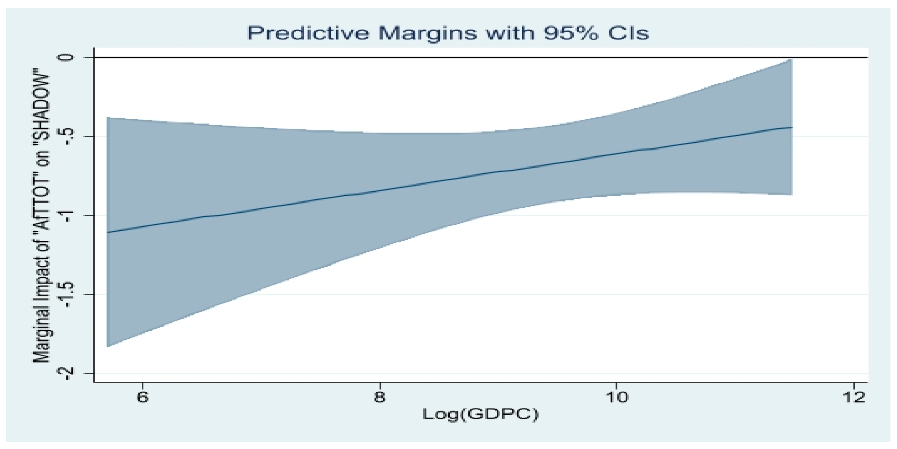
The results in column 5 of Table 2 indicate that the coefficient of the variable “AfTTOT” was negative and significant at the 5% level, while the interaction term of the variable [“Log(AfTTOT)]*[Log(GDPC)”] was still positive but not significant at the conventional significance levels. On the basis of these two outcomes, we were tempted to infer that the effect of the total AfT flows on the shadow economy was still negative but was not dependent on the countries’ development levels. To gain a better insight into this effect, we present the marginal impact of the total AfT flows on the shadow economy for varying levels of the real per capita income at the 95% confidence intervals in Figure 3. It appears in this figure that the marginal impact of the total AfT flows on the shadow economy was always negative and significant, but its magnitude (including in absolute value) diminished as the real per capita income rose. In other words, less developed countries experienced a larger negative effect of the total AfT flows on the shadow economy than relatively advanced economies among the recipient countries of AfT flows. We concluded that the total AfT flows were more effective in reducing the size of the shadow economy in less developed countries (including the poorest countries) than in relatively advanced countries.

Estimates related to control variables were, with few exceptions, broadly similar across all columns of Table 2. When focusing on the estimates in column 1 of Table 2, we obtained, as expected, that an increase in the real per capita income was negatively and significantly (at the 1% level) associated with the development of underground activities. The effect of burdensome taxes on the shadow economy was not significant at the conventional significance levels in column 1 of the table, but was, as expected, positive and significant at the 1% level in columns 4 and 5 of the table. We then inferred, as expected, that burdensome taxes tended to encourage the development of shadow activities. Greater financial development reduced the size of the shadow economy at least at the 5% level (see, for example, the results in columns 1, 4 and 5). Surprisingly, we obtained across all columns of Table 2 that at the 1% level, higher NonAfT flows and an improvement in the institutional and governance quality induced an expansion of the size of the shadow economy.

We suspected that the positive effect of the institutional and governance quality on the shadow economy may hide the existence of an interaction effect between the AfT flows (including the total AfT flows) and the institutional quality on the shadow economy. Our assumption was all the more relevant because Gnangnon (2020c) showed empirically that AfT flows could promote regulatory policies in recipient countries. We also suspected that the positive effect of the NonAfT flows on the shadow economy may reflect differentiated effects across countries in the full sample. It is for these reasons that we indicated in the previous section that Table 3 would report the outcomes concerning on one hand the extent to which the effect of the total AfT flows on the shadow economy depended on the quality of institutions and governance (see column 1 of Table 3), and on the other hand how the effect of the NonAfT flows on the shadow economy was conditioned on the countries’ level of real per capita income (see column 2 of Table 3).

Table 3. Effects of AfT flows and NonAfT flows, respectively, on the shadow economy for varying levels of the institutional and governance quality and varying levels of the real per capita income. Estimator: two-step system GMM.

Variables	SHADOW	SHADOW
	(1)	(2)
SHADOWt−1	0.537 ***	0.584 ***
	(0.0235)	(0.0281)
Log(AfTTOT)	−0.937 ***	−0.559 ***
	(0.218)	(0.178)
Log(NonAfT)	1.363 ***	6.281 ***
	(0.154)	(1.428)
[Log(AfTTOT)]*[INST]	−0.203 **
	(0.0892)
[Log(NonAfT)]*[Log(GDPC)]		−0.642 ***
		(0.170)
FINDEV	−0.0237 *	−0.0248 **
	(0.0139)	(0.0118)
INST	4.470 ***	0.576 **
	(1.435)	(0.283)
Log(GDPC)	−2.656 ***	10.22 ***
	(0.161)	(3.523)
TAXBURD	0.0301	0.0401 *
	(0.0270)	(0.0207)
Observations–Countries	276–106	276–106
Number of Instruments	69	69
AR1 (p-Value)	0.0270	0.0137
AR2 (p-Value)	0.2170	0.2147
OID (p-Value)	0.9040	0.6528

Note: * p-value < 0.1; ** p-value < 0.05; *** p-value < 0.01. Robust standard errors are in parentheses. All variables and the interaction variables were treated as endogenous. Time dummies were included in the regressions.

Table 3. Effects of AfT flows and NonAfT flows, respectively, on the shadow economy for varying levels of the institutional and governance quality and varying levels of the real per capita income. Estimator: two-step system GMM.

Variables	SHADOW	SHADOW
	(1)	(2)
SHADOWt−1	0.537 ***	0.584 ***
	(0.0235)	(0.0281)
Log(AfTTOT)	−0.937 ***	−0.559 ***
	(0.218)	(0.178)
Log(NonAfT)	1.363 ***	6.281 ***
	(0.154)	(1.428)
[Log(AfTTOT)]*[INST]	−0.203 **
	(0.0892)
[Log(NonAfT)]*[Log(GDPC)]		−0.642 ***
		(0.170)
FINDEV	−0.0237 *	−0.0248 **
	(0.0139)	(0.0118)
INST	4.470 ***	0.576 **
	(1.435)	(0.283)
Log(GDPC)	−2.656 ***	10.22 ***
	(0.161)	(3.523)
TAXBURD	0.0301	0.0401 *
	(0.0270)	(0.0207)
Observations–Countries	276–106	276–106
Number of Instruments	69	69
AR1 (p-Value)	0.0270	0.0137
AR2 (p-Value)	0.2170	0.2147
OID (p-Value)	0.9040	0.6528

Note: * p-value < 0.1; ** p-value < 0.05; *** p-value < 0.01. Robust standard errors are in parentheses. All variables and the interaction variables were treated as endogenous. Time dummies were included in the regressions.

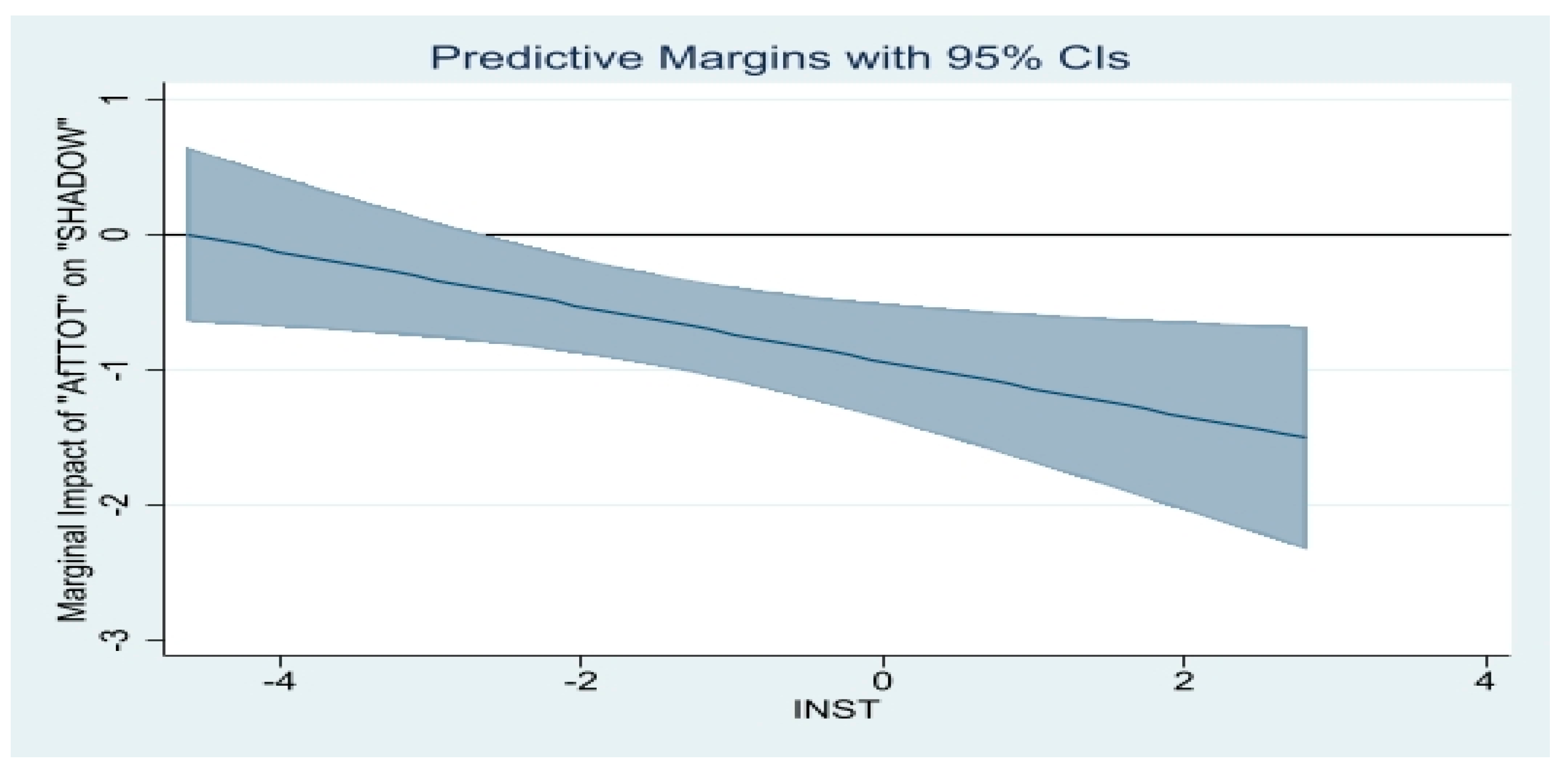
Column 1 of Table 3 shows that both the coefficient of the variable [“Log(AfTTOT)”] and the interaction term of the interaction variable (“[Log(AfTTOT)]*INST”) were negative and significant at the 1% level and the 5% level, respectively. We concluded that on average over the full sample, the total AfT flows always reduced the size of the shadow economy regardless of the quality of institutions and governance. The magnitude of this reduction effect on the shadow economy increased as countries improved their institutional and governance quality. Figure 4 shows the marginal impact of the total AfT flows on the shadow economy for varying levels of the quality of institutions and governance at the 95% confidence intervals. It appears in this figure that in countries with weak institutional and governance quality (especially when the values of the variable “INST5“ were lower than −2.643), there was no significant effect of the total AfT flows on the shadow economy. However, for the other countries, the total AfT flows exerted a negative effect on the shadow economy, and the magnitude of this reducing effect became larger as the institutional and governance quality improved.

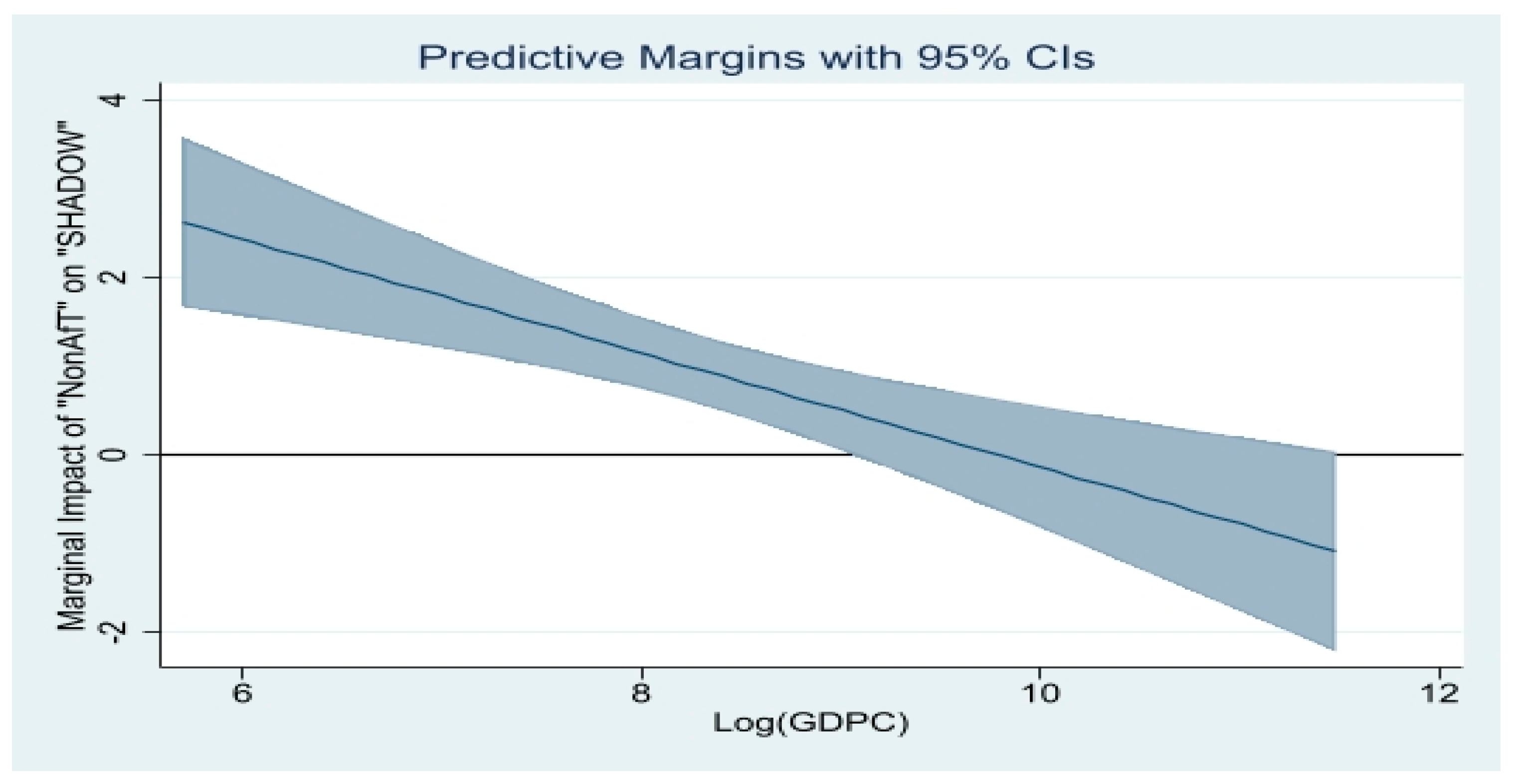
Column 2 of Table 3 shows that the coefficient of the variable [“Log(NonAfT)”] was positive and significant at the 1% level, while the interaction variable (“[Log(NonAfT)]*[Log(GDPC)]”) was negative and significant at the 1% level. These two outcomes suggested that NonAfT flows reduced the shadow economy in countries with a real per capita income6 that exceeded USD 17738.44 (=exponential (6.281/0.642)). Otherwise, higher NonAfT flows led to an expansion of the shadow economy. We obtained a better picture of this effect as displayed in Figure 5, which shows the marginal impact of the total NonAfT flows on the shadow economy for varying levels of the real per capita income at the 95% confidence intervals. This figure shows that the marginal impact of the NonAfT flows on the shadow economy was positive and significant only for countries with a real per capita income lower than USD 8148.70. For these countries, the lower the real per capita income, the higher the magnitude of the positive effect of the NonAfT flows on the shadow economy. In other words, among countries that had a real per capita income lower than USD$ 8148.70, poor countries experienced a higher positive effect of the NonAfT flows on the shadow economy than other countries. In contrast, countries with a real per capita income that exceeded USD 8148.70 experienced no significant effect of the NonAfT flows on the shadow economy. The positive effect of the NonAfT flows on the shadow economy may also reflect the fact that this effect worked through the real exchange rate appreciation. In other words, it was possible that the real exchange appreciation effect of NonAfT flows on the shadow economy likely dominated the eventual negative effects that these resources inflows may have exerted on the shadow economy; for example, through human capital accumulation. We will test the extent to which NonAfT flows affected the shadow economy through the real exchange rate avenue later in the analysis.

We now consider the outcomes reported in Table 4. Column 1 of this table shows that the introduction of the trade costs indicator led to a diminution of the magnitude of the effect of the total AfT flows on the shadow economy from a value of −0.73 (see column 1 of Table 2) to a value of −1.533 in column 1 of Table 4. In other words, while the coefficient of the variable “AfTTOT” remained significant at the 1% level in column 1 of Table 4, its magnitude was diminished after the introduction of the indicator of the overall trade costs. This suggested that trade costs were genuinely a channel through which the AfT flows affected the shadow economy. Incidentally, as expected, higher trade costs induced an expansion of the underground activities (at the 1% level). This positive and significant effect of trade costs on the shadow economy was confirmed by the data in all other columns of Table 4 at least at the 5% level. The coefficients of the AfT indicators (the total AfT or each of its components) were positive and significant at least at the 10% level across columns 2 to 5 of Table 4. Concurrently, the interaction terms of the multiplicative variable between each of these AfT indicators and the trade costs indicator were all negative and significant at least at the 5% level. These outcomes suggested that on average over the full sample, the AfT flows tended to exert a negative effect on the shadow economy in countries that faced high trade costs, notably those with overall trade costs7 that were higher than 185.2 (=exponential(11.90/2.279)) for the shadow economy effect of the total AfT flows, higher than 143.8 (=exponential(5.768/1.161)) for the shadow economy effect of the AfT interventions for economic infrastructure, higher than 269.4 (=exponential(18.02/3.220)) for the shadow economy effect of the AfT interventions for productive capacities, and higher than 284.4 (=exponential(31.53/5.580)) for the shadow economy effect of the AfT interventions for trade policy and regulation. For trade costs lower than these levels, the relevant AfT indicator positively influenced the shadow economy. These outcomes tended to suggest that the AfT flows reduced the shadow economy in countries that faced high trade costs and that the greater the trade costs (especially when they exceed the above-mentioned levels), the larger the magnitude of the negative effect of the relevant AfT intervention on the shadow economy.

Table 4. Effects of AfT flows on the shadow economy. Estimator: two-step system GMM.

Variables	SHADOW	SHADOW	SHADOW	SHADOW	SHADOW
	(1)	(2)	(3)	(4)	(5)
SHADOWt−1	0.788 ***	0.779 ***	0.757 ***	0.760 ***	0.704 ***
	(0.0363)	(0.0284)	(0.0271)	(0.0271)	(0.0226)
Log(AfTTOT)	−1.533 ***	11.90 **
	(0.306)	(5.422)
Log(TRCOST)	4.883 ***	45.81 ***	25.39 **	59.60 ***	78.85 ***
	(1.795)	(17.35)	(10.03)	(12.84)	(13.46)
[Log(AfTTOT)]*[ Log(TRCOST)]		−2.279 **
		(0.933)
Log(AfTINFRA)			5.768 *
			(3.214)
[Log(AfTINFRA)]*[ Log(TRCOST)]			−1.161 **
			(0.564)
Log(AfTPROD)				18.02 ***
				(4.099)
[Log(AfTPROD)]*[ Log(TRCOST)]				−3.220 ***
				(0.715)
Log(AfTPOL)					31.53 ***
					(5.432)
[Log(AfTPOL)]*[ Log(TRCOST)]					−5.580 ***
					(0.934)
Log(NonAfT)	1.915 ***	1.907 ***	1.351 ***	1.156 ***	1.770 ***
	(0.436)	(0.372)	(0.417)	(0.286)	(0.372)
FINDEV	−0.0448 ***	−0.0545 ***	−0.0477 ***	−0.0678 ***	−0.0490 ***
	(0.0137)	(0.0109)	(0.00759)	(0.0127)	(0.0115)
INST	1.471 ***	1.580 ***	1.490 ***	1.280 ***	1.081 ***
	(0.439)	(0.368)	(0.312)	(0.396)	(0.362)
Log(GDPC)	−0.441	−0.633 **	−0.494 *	−0.585 **	−1.045 ***
	(0.331)	(0.278)	(0.280)	(0.252)	(0.284)
TAXBURD	0.0806 ***	0.0521 **	0.0315	0.0514 **	0.0501 *
	(0.0282)	(0.0261)	(0.0308)	(0.0219)	(0.0259)
Observations–Countries	251–96	251–96	250–95	251–96	245–94
Number of Instruments	54	60	61	61	61
AR1 (p-Value)	0.0215	0.0236	0.0183	0.0229	0.0224
AR2 (p-Value)	0.3005	0.2313	0.2862	0.1865	0.3734
OID (p-Value)	0.7368	0.5669	0.7373	0.5167	0.8248

Note: * p-value < 0.1; ** p-value < 0.05; *** p-value < 0.01. Robust standard errors are in parentheses. All variables and the interaction variables were treated as endogenous. Time dummies were included in the regressions.

Table 4. Effects of AfT flows on the shadow economy. Estimator: two-step system GMM.

Variables	SHADOW	SHADOW	SHADOW	SHADOW	SHADOW
	(1)	(2)	(3)	(4)	(5)
SHADOWt−1	0.788 ***	0.779 ***	0.757 ***	0.760 ***	0.704 ***
	(0.0363)	(0.0284)	(0.0271)	(0.0271)	(0.0226)
Log(AfTTOT)	−1.533 ***	11.90 **
	(0.306)	(5.422)
Log(TRCOST)	4.883 ***	45.81 ***	25.39 **	59.60 ***	78.85 ***
	(1.795)	(17.35)	(10.03)	(12.84)	(13.46)
[Log(AfTTOT)]*[ Log(TRCOST)]		−2.279 **
		(0.933)
Log(AfTINFRA)			5.768 *
			(3.214)
[Log(AfTINFRA)]*[ Log(TRCOST)]			−1.161 **
			(0.564)
Log(AfTPROD)				18.02 ***
				(4.099)
[Log(AfTPROD)]*[ Log(TRCOST)]				−3.220 ***
				(0.715)
Log(AfTPOL)					31.53 ***
					(5.432)
[Log(AfTPOL)]*[ Log(TRCOST)]					−5.580 ***
					(0.934)
Log(NonAfT)	1.915 ***	1.907 ***	1.351 ***	1.156 ***	1.770 ***
	(0.436)	(0.372)	(0.417)	(0.286)	(0.372)
FINDEV	−0.0448 ***	−0.0545 ***	−0.0477 ***	−0.0678 ***	−0.0490 ***
	(0.0137)	(0.0109)	(0.00759)	(0.0127)	(0.0115)
INST	1.471 ***	1.580 ***	1.490 ***	1.280 ***	1.081 ***
	(0.439)	(0.368)	(0.312)	(0.396)	(0.362)
Log(GDPC)	−0.441	−0.633 **	−0.494 *	−0.585 **	−1.045 ***
	(0.331)	(0.278)	(0.280)	(0.252)	(0.284)
TAXBURD	0.0806 ***	0.0521 **	0.0315	0.0514 **	0.0501 *
	(0.0282)	(0.0261)	(0.0308)	(0.0219)	(0.0259)
Observations–Countries	251–96	251–96	250–95	251–96	245–94
Number of Instruments	54	60	61	61	61
AR1 (p-Value)	0.0215	0.0236	0.0183	0.0229	0.0224
AR2 (p-Value)	0.3005	0.2313	0.2862	0.1865	0.3734
OID (p-Value)	0.7368	0.5669	0.7373	0.5167	0.8248

Note: * p-value < 0.1; ** p-value < 0.05; *** p-value < 0.01. Robust standard errors are in parentheses. All variables and the interaction variables were treated as endogenous. Time dummies were included in the regressions.

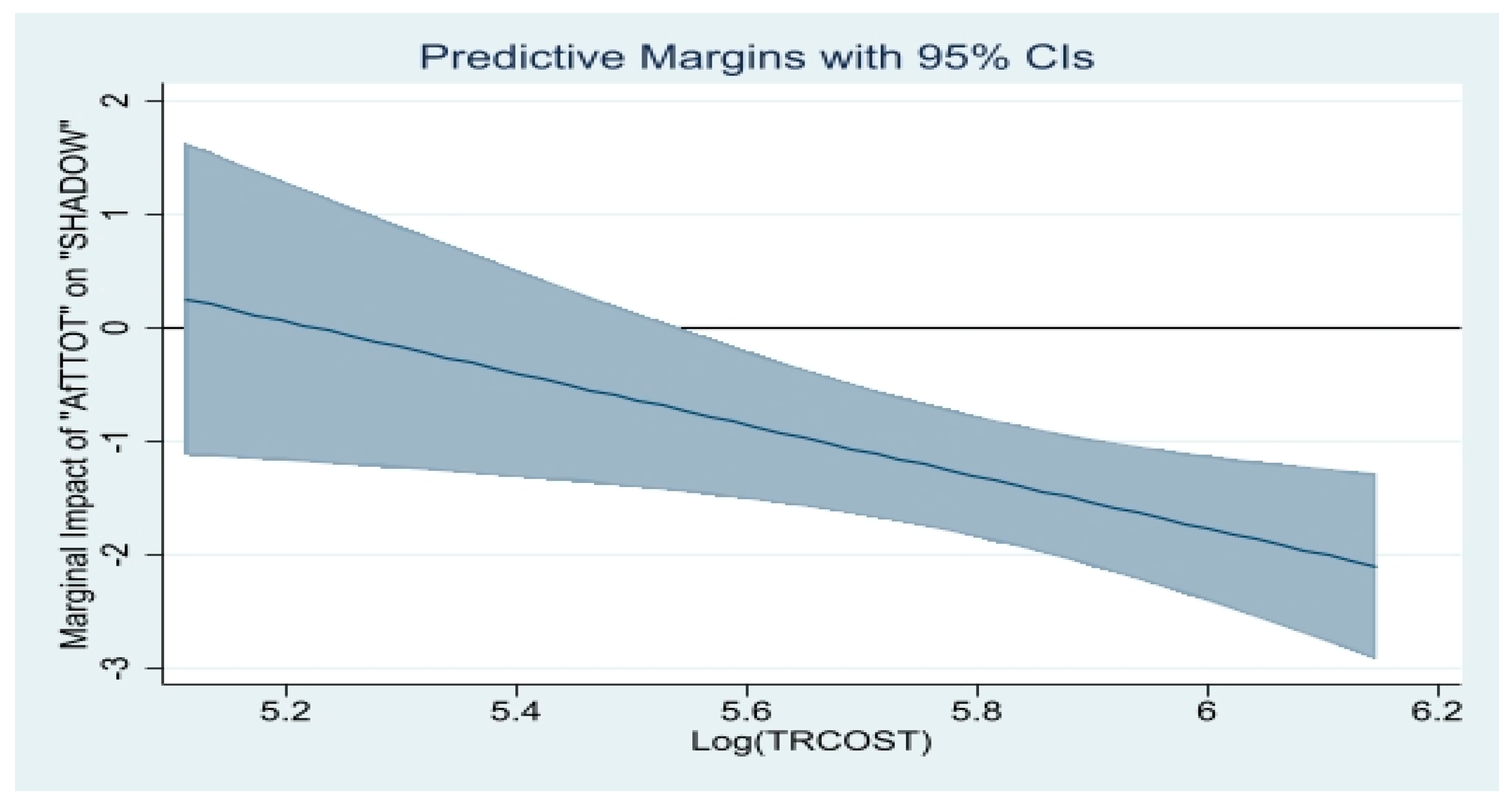
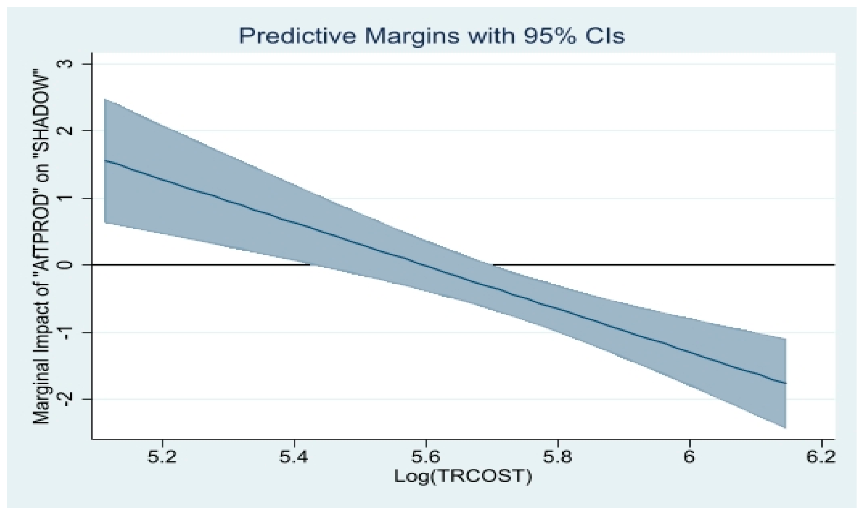
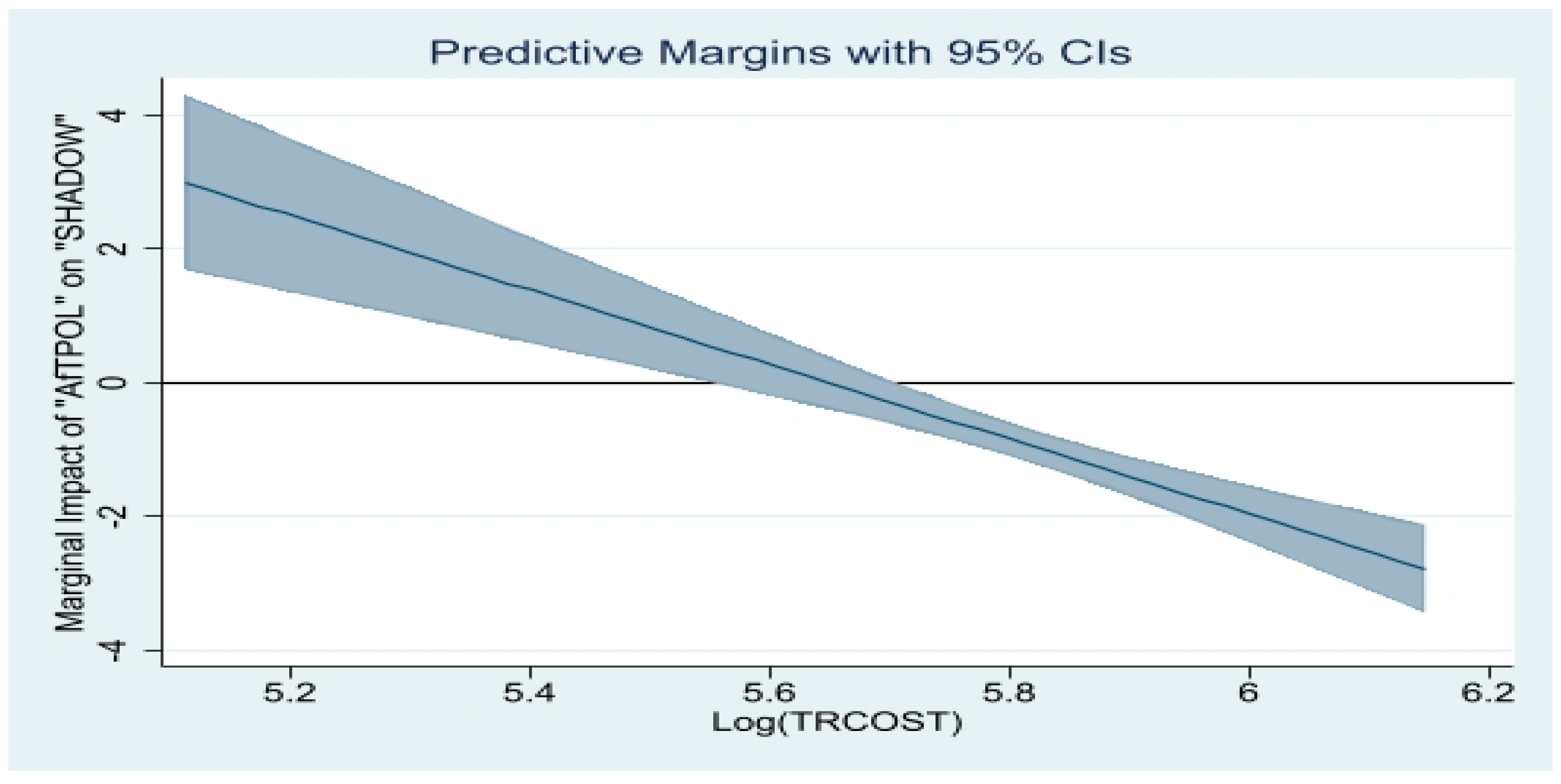
To gain a better insight into these effects, we provide the respective marginal impact of the total AfT flows, AfT flows for economic infrastructure, AfT flows for productive capacities, and AfT flows for trade policy and regulation on the shadow economy for varying levels of trade costs at the 95% confidence intervals in Figure 6, Figure 7, Figure 8 and Figure 9. We note that in all four of these figures, the marginal impact of a relevant AfT indicator on the shadow economy decreased as the overall trade costs increased. However, this marginal impact was not always statistically significant. In particular, when this marginal impact was significant, the relevant AfT flows exerted a negative effect on the shadow economy, and the larger the magnitude of this negative effect, the higher the overall trade costs. Specifically, we observed that total AfT flows exerted no significant effect on the shadow economy in countries that faced trade costs that were lower than 256.5 (see Figure 6). However, for countries with overall trade costs that exceeded 256.5, the total AfT flows led to a reduction in the size of the shadow economy. A similar pattern can be observed in Figure 7, which shows that the marginal effect of the AfT interventions for economic infrastructure were statistically nil when the trade costs were lower than 236.2 and statistically significant for higher trade costs. Figure 8 also shows that the marginal effect of the AfT interventions for productive capacities on the shadow economy was negative and significant for trade costs higher than 296.5. Otherwise, this marginal effect was at best statistically nil (for trade costs ranging from 231.3 to 296.5) or positive when the trade costs were lower than 231.3.

Figure 9 displays a pattern similar to the one shown in Figure 8: the marginal effect of the AfT interventions for trade policy and regulation on the shadow economy was negative and significant for trade costs higher than 302.7. For countries facing levels of overall trade costs lower than 261.9, the AfT interventions related to trade policy and regulation induced an expansion of the shadow economy. Countries with trade costs that ranged from 261.9 to 302.7 experienced no significant effect of the AfT interventions for trade policy and regulation on the shadow economy.

Overall, the results shown in Table 4 and the related Figure 6, Figure 7, Figure 8 and Figure 9 indicated that the AfT flows, including the total AfT flows and the major components thereof, reduced the size of the shadow economy in countries that faced high trade costs: the greater the overall trade costs, the larger the negative shadow economy effect of the AfT flows. These findings gave credence to Hypothesis 1.

The estimates related to the control variables in Table 4 were consistent with those in Table 2.

Taking up the outcomes in Table 5, we note in column 1 that while the coefficient of the variable “REER” was not significant at the 10% level, its introduction in the baseline dynamic model (1) led to a diminution in the magnitude of the coefficient of “AfTTOT” from a value of −0.73 (in column 1 of Table 2) to a value of −1.542 (see column 1 of Table 5). These outcomes indicated that the real exchange rate was another channel through which the total AfT flows could affect the shadow economy. We note in the results in column 2 of Table 5 that the coefficient of the variable “Log(REER)” was positive but not significant at the 10% level. At the same time, the interaction term of the variable (“[Log(AfTTOT)]*[Log(REER)]”) was positive and significant at the 1% level, and the interaction term of the variable (“[Log(NonAfT)]*[Log(REER)]”) was negative and significant at the 1% level. These outcomes indicated that the effects of both the total AfT flows and NonAfT flows on the shadow economy depended on the real exchange rate, with these effects moving in opposite directions as the real exchange rate appreciated. Specifically, the total AfT flows induced a reduction in underground activities in countries that experienced a depreciation in the real exchange rate: for these countries, the higher the depreciation in the real exchange rate, the larger the magnitude of the negative effect of the total AfT flows on the shadow economy. NonAfT flows induced an expansion of the shadow economy in countries that experienced an appreciation in the real exchange rate, and the magnitude of this positive shadow economy effect increased as the real exchange rate further appreciated.

Table 5. Effects of AfT flows on the shadow economy conditioned on the real exchange rate. Estimator: two-step system GMM.

Variables	SHADOW	SHADOW
	(1)	(2)
SHADOWt−1	0.870 ***	0.748 ***
	(0.0296)	(0.0165)
Log(AfTTOT)	−1.542 ***	−18.44 ***
	(0.276)	(3.881)
Log(REER)	0.206	3.736
	(1.871)	(13.02)
[Log(AfTTOT)]*[Log(REER)]		3.662 ***
		(0.827)
[Log(NonAfT)]*[Log(REER)]		−3.654 ***
		(1.105)
Log(NonAfT)	2.947 ***	18.98 ***
	(0.457)	(5.145)
FINDEV	−0.0133	−0.00733
	(0.0155)	(0.0115)
INST	1.425 ***	0.487 **
	(0.329)	(0.229)
Log(GDPC)	−1.117 ***	−1.849 ***
	(0.328)	(0.238)
TAXBURD	−0.0231	0.0374 *
	(0.0278)	(0.0208)
Observations–Countries	267–102	267–102
Number of Instruments	54	64
AR1 (p-Value)	0.0437	0.0407
AR2 (p-Value)	0.6484	0.3907
OID (p-Value)	0.8190	0.5944

Note: * p-value < 0.1; ** p-value < 0.05; *** p-value < 0.01. Robust standard errors are in parentheses. All variables and the interaction variables were treated as endogenous. Time dummies were included in the regressions.

Table 5. Effects of AfT flows on the shadow economy conditioned on the real exchange rate. Estimator: two-step system GMM.

Variables	SHADOW	SHADOW
	(1)	(2)
SHADOWt−1	0.870 ***	0.748 ***
	(0.0296)	(0.0165)
Log(AfTTOT)	−1.542 ***	−18.44 ***
	(0.276)	(3.881)
Log(REER)	0.206	3.736
	(1.871)	(13.02)
[Log(AfTTOT)]*[Log(REER)]		3.662 ***
		(0.827)
[Log(NonAfT)]*[Log(REER)]		−3.654 ***
		(1.105)
Log(NonAfT)	2.947 ***	18.98 ***
	(0.457)	(5.145)
FINDEV	−0.0133	−0.00733
	(0.0155)	(0.0115)
INST	1.425 ***	0.487 **
	(0.329)	(0.229)
Log(GDPC)	−1.117 ***	−1.849 ***
	(0.328)	(0.238)
TAXBURD	−0.0231	0.0374 *
	(0.0278)	(0.0208)
Observations–Countries	267–102	267–102
Number of Instruments	54	64
AR1 (p-Value)	0.0437	0.0407
AR2 (p-Value)	0.6484	0.3907
OID (p-Value)	0.8190	0.5944

Note: * p-value < 0.1; ** p-value < 0.05; *** p-value < 0.01. Robust standard errors are in parentheses. All variables and the interaction variables were treated as endogenous. Time dummies were included in the regressions.

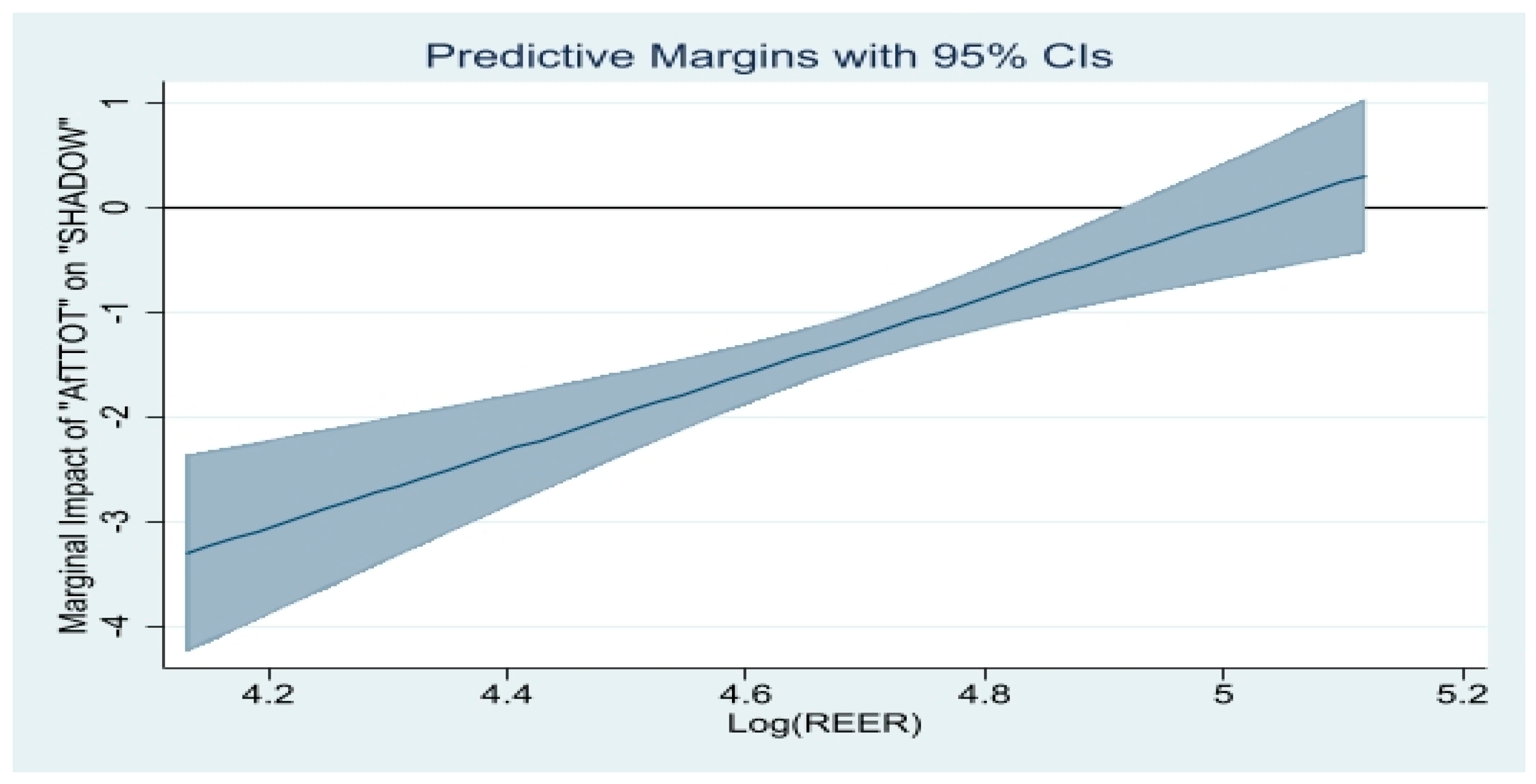
These findings are illustrated in Figure 10 and Figure 11, which present the marginal impact of the total AfT flows and NonAfT flows, respectively, on the shadow economy conditioned on the real exchange rate at the 95% confidence intervals. Figure 10 indicates that the marginal effect of the total AfT flows on the shadow economy increased as the real exchange rate appreciated. It was not statistically significant for values of the real exchange rate8 that exceeded 137.2. Conversely, countries with levels of the real exchange rate that were below 137.2 experienced a negative and significant effect of the total AfT flows on the shadow economy, and the larger the magnitude of this negative effect, the lower the value of the real exchange rate (i.e., the larger the depreciation in the real exchange rate). These findings clearly supported Hypothesis 2.

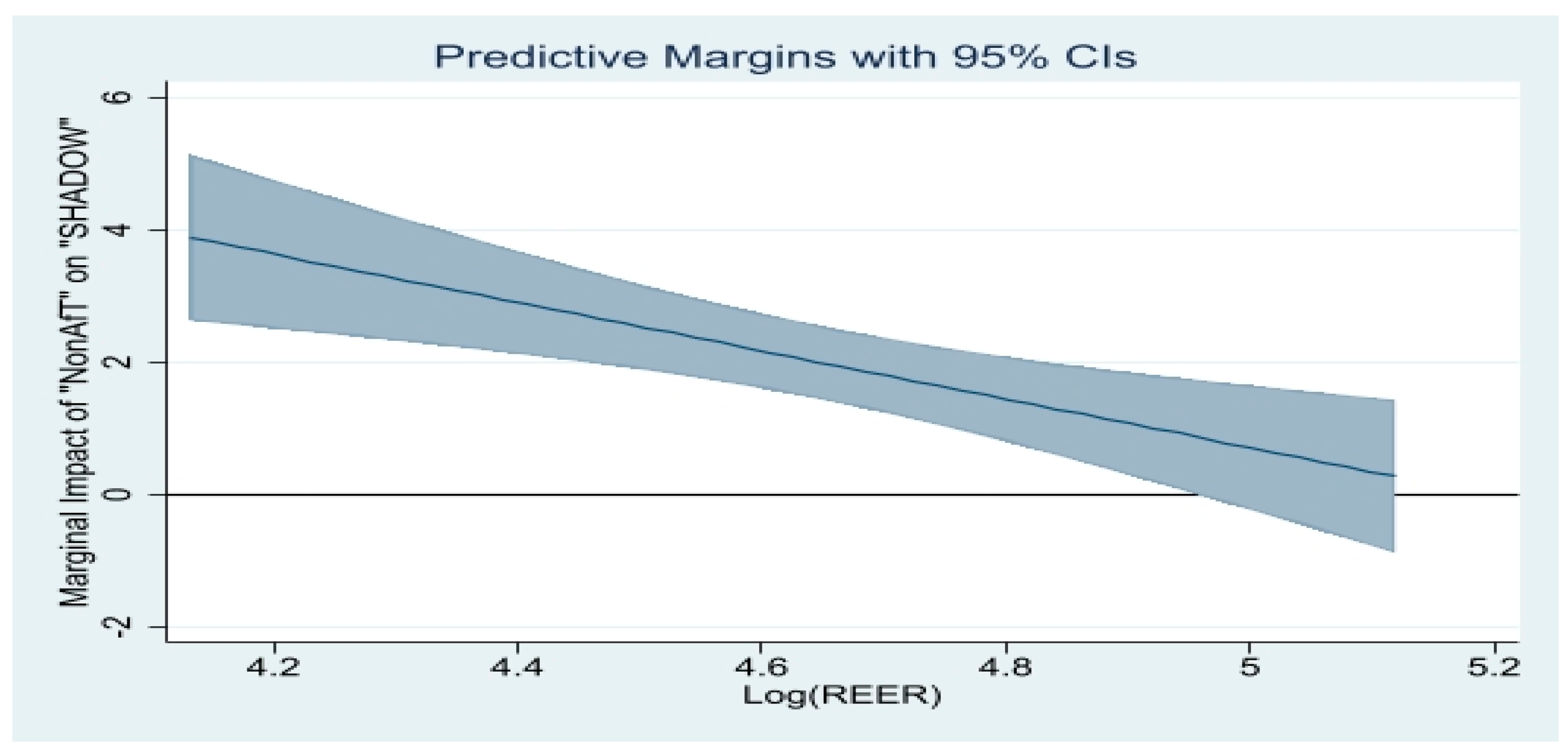
On the other hand, Figure 11 shows that the marginal effect of the NonAfT flows on the shadow economy was always positive, in particular when it was significant. This marginal effect was not significant for values of the real exchange rate higher than 142.7. For lower levels of the real exchange rate, the NonAfT flows exerted a positive and significant effect on the shadow economy as the real exchange rate appreciated, and the greater the appreciation in the real exchange rate, the higher the shadow economy expansion effect of the NonAfT flows.

In sum, the results shown in Table 5 and in the related Figure 10 and Figure 11 convey the message that while the total AfT flows reduced the shadow economy through their real exchange rate depreciation effect, higher NonAfT flows were associated with an expansion of underground economies through their real exchange rate appreciation effect. This finding concerning NonAfT flows helped us to better understand why we obtained the data in Table 3 showing that the NonAfT flows exerted a positive effect on the shadow economy.

7. Further Analysis

The previous analysis demonstrated empirically that the AfT interventions exerted a higher negative effect on the shadow economy in countries that faced higher trade costs than in countries that faced relatively lower trade costs. This section deepens the analysis by investigating whether the effect of the AfT flows on the shadow economy depended on the countries’ level of economic sophistication, including their level of economic complexity. The complexity of an economy is defined by the current stage of its production knowledge or the knowledge materialized in the production system (e.g., Hausmann and Hidalgo 2009; Hausmann et al. 2014). Thus, a complex economy features a high level of diversity of export products and a low ubiquity of these products9 (e.g., Hartmann et al. 2017; Hausmann and Hidalgo 2009; Hausmann et al. 2014; Mishra et al. 2020).

The relevance of the question addressed in this section lies in the fact that on one hand, higher trade costs undermine export upgrading (including improvements in export product quality and export product diversification) (e.g., Bas and Strauss-Kahn 2015; Beverelli et al. 2015; Chen and Juvenal 2022; Dennis and Shepherd 2011) and more generally hinder countries’ ability to produce and export sophisticated products (e.g., Hu et al. 2022; Weldemicael 2014), while on the other hand, Nguyen (2022) found empirically that an improvement in the economic complexity level reduces the size of the shadow economy in the long run. In light of the foregoing, one could expect that by reducing trade costs and encouraging the export of complex products, AfT flows could help limit the development of underground activities insofar as economic complexity has a negative effect on the size of the shadow economy. Overall, we postulated that AfT interventions would reduce the size of the shadow economy in economies that became increasingly sophisticated (Hypothesis 4).

To empirically test Hypothesis 4, we used two different indicators of economic sophistication. The first one was denoted “ECONC” and reflected the diversity and ubiquity of a country’s export structure. It was estimated using the data that connected countries to the exported products and by applying the methodology described in Hausmann and Hidalgo (2009). Higher values of this indicator reflected a greater economic complexity (see Table A1 for details on this indicator). The second indicator (denoted “PCI”) was the level of productive capacities of a given country and represented “the productive resources, entrepreneurial capabilities and production linkages which together determine the capacity of a country to produce goods and services and enable it to grow and develop” (e.g., UNCTAD 2006, p61, 2020). It was computed as a geometric average of eight components; namely, information communication and technologies, structural change, natural capital, human capital, energy, transport, the private sector, and institutions (see UNCTAD 2020). Its values ranged between 0 and 100; greater values reflected greater productive capacities (see Table A1 for details on this indicator).

We estimated a first variant of model (1); that is, model (1) but in which we incorporated the indicator of economic sophistication10. This specification of model (1) allowed us to check whether economic sophistication was a channel through which AfT interventions could affect the shadow economy. Put differently, we expected here that the introduction of the economic sophistication indicator in the baseline specification of model (1) would alter the coefficient of the variable “AfTTOT” (in Log) shown in column 1 of Table 2 by either by diminishing the magnitude of this coefficient (which would remain significant at least at the 5% level—or eventually at the 10% level) or by cancelling out its statistical significance at the 5% level (or eventually at the 10% level). Columns 1 and 2 of

Table 6. Effects of AfT flows on the shadow economy conditioned on export product diversification/economic sophistication. Estimator: two-step system GMM.

Variables	SHADOW	SHADOW	SHADOW	SHADOW
	(1)	(2)	(3)	(4)
SHADOWt−1	0.720 ***	0.811 ***	0.650 ***	0.752 ***
	(0.0284)	(0.0294)	(0.0320)	(0.0246)
Log(AfTTOT)	0.181	−0.150	−0.668 **	2.299 ***
	(0.245)	(0.144)	(0.317)	(0.744)
ECONC	−2.706 ***		9.776 **
	(0.720)		(3.937)
PCI		−0.180 ***		1.769 ***
		(0.0588)		(0.521)
[Log(AfTTOT)]*ECONC			−0.588 ***
			(0.205)
[Log(AfTTOT)]*PCI				−0.0961 ***
				(0.0274)
Log(NonAfT)	0.678	−0.203	0.997 **	0.655
	(0.471)	(0.239)	(0.409)	(0.410)
FINDEV	−0.0221		−0.0528 ***
	(0.0150)		(0.0130)
INST	0.178		0.425
	(0.430)		(0.497)
Log(GDPC)	−1.495 ***	−1.035 ***	−1.794 ***	−0.940 ***
	(0.282)	(0.276)	(0.340)	(0.227)
TAXBURD	0.0588 ***	0.107 ***	0.0995 ***	0.0714 ***
	(0.0197)	(0.0243)	(0.0203)	(0.0251)
Observations–Countries	224–83	270–101	224–83	270–101
Number of Instruments	54	52	58	49
AR1 (p-Value)	0.0242	0.0335	0.0271	0.0385
AR2 (p-Value)	0.4779	0.6738	0.5750	0.5427
OID (p-Value)	0.5632	0.2481	0.3818	0.6720

Note: * p-value < 0.1; ** p-value < 0.05; *** p-value < 0.01. Robust Standard Errors are in parentheses. All variables and the interaction variables were treated as endogenous. Time dummies were included in the regressions. Note that the specifications of model (1), the results of which are reported in columns 2 and 4, did not contain the variables “FINDEV” and “INST”, as these variables were components of the productive capacities indicator.

report the outcomes obtained from the estimation of this variant of model (1) (by means of the two-step system GMM estimator) using “ECONC” and “PCI” as the measures of economic sophistication.

Second, we used the two-step system GMM estimator to estimate another specification of model (1) that contained the multiplicative variable between the indicator of total AfT flows and the indicator of economic sophistication (i.e., alternatively “ECONC” and “PCI”). This specification of model (1) helped to test Hypothesis 4; i.e., to examine the extent to which the effect of the total AfT flows on the shadow economy was conditioned on economic sophistication. The outcomes of the estimation are presented in columns 3 and 4 of Table 6. Note that the specifications of model (1) in which “PCI” was the measure of economic sophistication did not contain the variables “FINDEV” and “INST” because these variables were components of the productive capacities index (see the results in columns 2 and 4 of Table 6).

We note that in all four columns of Table 6, the coefficients of the lagged dependent variable were positive and significant at the 1% level, thereby suggesting the existence of a state-dependent path of the shadow economy indicator. These outcomes validated the dynamic nature of the model specifications, the results of which are reported in these columns of Table 6. In addition, these models were correctly specified as exemplified by the outcomes of the diagnostic tests, the results of which are reported at the bottom of the table. Thus, once again, the two-step system GMM estimator was very appropriate for the empirical analysis outlined in this section.

The outcomes shown in columns 1 and 2 of Table 6 revealed that the introduction of the economic complexity indicator (either “ECONC” or “PCI”) in the baseline model (1) rendered the coefficient of the variable “AfTTOT” statistically nil at the conventional significance levels. To recall, the coefficient of this variable in column 1 of Table 2 was significant at the 1% level and amounted to −0.731. We concluded that the economic complexity measured either by the indicator “ECONC” or by “PCI” represented a channel through which the AfT flows could affect the shadow economy.

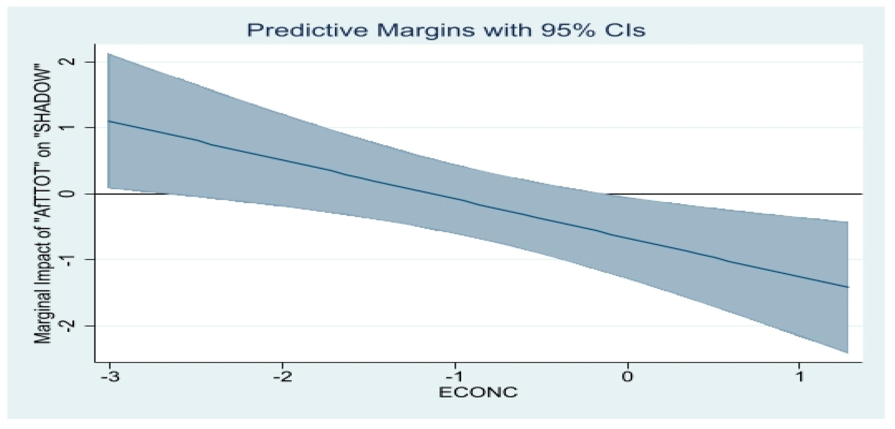
Turning to the outcomes shown in column 3, we observed that both the coefficient of the variable [“Log(AfTTOT)”] and the interaction term of the variable (“[Log(AfTTOT)]*ECONC”) were negative, with the former being significant at the 5% level and the latter being significant at the 1% level. We concluded that on average over the full sample, the effect of the total AfT flows on the shadow economy depended on the countries’ level of economic complexity: AfT interventions were consistently associated with a reduction in the size of the shadow economy, and the magnitude of this negative effect increased (in absolute value) as the countries increasingly exported complex products; i.e., as their level of economic complexity improved. Figure 12 displays the marginal impact of the total AfT flows on the shadow economy conditioned on the level of economic complexity at the 95% confidence intervals. It appears that the total AfT flows led to an increase in the size of the shadow economy in countries with low levels of economic complexity (for example, this was the case of poor countries), especially in countries with a level of economic complexity11 lower than −2.67. In contrast, AfT interventions resulted in a reduction in the shadow economy size in countries with a level of economic complexity that was higher than −0.18: for these countries, the higher the degree of economic complexity, the larger the reduction in the shadow economy size. Finally, countries with a level of economic complexity that ranged between −2.67 and −0.18 experienced no significant effect of the total AfT flows on the shadow economy.

The estimates given in column 4 of Table 6 show that the coefficient of [Log(AfTTOT)] was positive and significant at the 1% level, while the interaction term of the variable (“[Log(AfTTOT)]*PCI”) was negative and significant at the 1% level. When combined, these two results suggested that the effect of AfT flows on the shadow economy depended on the recipient countries’ level of productive capacities. On average over the full sample, AfT interventions contributed to reducing the size of the shadow economy in countries with a level of productive capacities12 that was higher than 18.4 (=1.769/0.0961) but led to an expansion of the shadow economy in countries that had weak productive capacities (i.e., those with a level of productive capacities that was lower than 18.4—for example, poor countries).

Figure 13 shows the marginal impact of the total AfT flows on the shadow economy conditioned on the level of productive capacities at the 95% confidence intervals. The pattern of the graph in this figure is similar to the one observed in Figure 12. AfT interventions led to an expansion of the shadow economy in countries with weak productive capacities; i.e., those with a level of productive capacities that was lower than 17.7. In contrast, these resource flows reduced the size of the shadow economy in countries that had relatively strong productive capacities; that is, those with a level of productive capacities that exceeded the value of 28.2. For these countries, the stronger the productive capacities, the larger the reduction effect of the AfT interventions on the shadow economy. Finally, there was no significant effect of AfT interventions on the shadow economy in countries with a level of productive capacities that ranged between −17.7 and 28.2.

8. Conclusions

Numerous studies have examined the drivers of the shadow economy. However, the shadow economy effect of development aid, let alone that of AfT flows, has received little attention in the literature. The present analysis investigated the effect of AfT flows on the shadow economy using an unbalanced panel dataset of 106 countries over the period of 2002 to 2015. It established empirically that over the full sample, higher AfT flows led to a reduction in the size of the shadow economy. Among recipient countries of AfT flows, less developed countries enjoyed a greater negative effect of AfT flows on the shadow economy than relatively advanced countries. Moreover, the negative effect of AfT flows on the shadow economy was larger in countries that faced high trade costs, and the higher the overall trade costs, the larger the magnitude of the negative effect of the AfT flows on trade costs. The analysis also revealed that AfT flows induced a shrinking of the shadow activities in countries that experienced a depreciation in the real exchange rate, and the greater the depreciation in the real exchange rate, the larger the negative shadow economy effect of the total AfT flows. Finally, AfT interventions reduced the size of the shadow economy in countries that exported increasingly complex products and in those that enhanced their level of productive capacities.

These findings complemented the existing works on the determinants of the shadow economy by showing that AfT interventions contributed significantly to reducing the size of the shadow economy in recipient countries. Participation in international trade promotes economic growth and development under certain conditions (e.g., Atkin and Donaldson 2022; Singh 2010), and AfT interventions can help enhance countries’ participation in international trade (e.g., Benziane et al. 2022). In particular, AfT flows could allow recipient countries to reduce trade costs, upgrade exports, and ultimately reduce the size of the informal sector. It follows that greater financial support of developing countries by the international trade community through higher AfT flows would help developing countries reduce their underground activities. In turn, the resulting expansion of the formal sector could lead to higher public revenues and reduce countries’ dependence on AfT flows in the medium term.

References

1. Abeberese, Ama Baafra, and Mary Chen. 2022. Intranational trade costs, product scope and productivity: Evidence from India’s Golden Quadrilateral project. Journal of Development Economics 156: 102791. [Google Scholar] [CrossRef]
2. Afonso, Oscar, Pedro Cunha Neves, and Tiago Pinto. 2020. The non-observed economy and economic growth: A meta-analysis. Economic Systems 44: 100746. [Google Scholar] [CrossRef]
3. Aggarwal, Shilpa, Brian Giera, Dahyeon Jeong, Jonathan Robinson, and Alan Spearot. 2022. Market Access, Trade Costs, and Technology Adoption: Evidence from Northern Tanzania. Paper formally published in 2018 as Working Paper 25253, NBER, Cambridge, MA—and updated in 2022. Available online: https://people.ucsc.edu/~jmrtwo/market_access.pdf (accessed on 17 October 2022).
4. Ali, Salamat, and Chris Milner. 2016. Narrow and Broad Perspectives on Trade Policy and Trade Costs: How to Facilitate Trade in Madagascar. The World Economy 39: 1917–33. [Google Scholar] [CrossRef] [Green Version]
5. Alonso-Borrego, Cesar, and Manuel Arellano. 1999. Symmetrically normalized instrumental-variable estimation using panel data. Journal of Business & Economic Statistics 17: 36–49. [Google Scholar]
6. Anderson, James E., and Douglas Marcouiller. 2002. Insecurity and the pattern of trade: An empirical investigation. Review of Economics and Statistics 84: 342–52. [Google Scholar] [CrossRef] [Green Version]
7. Anderson, James E., and Eric Van Wincoop. 2004. Trade Costs. Journal of Economic Literature 42: 691–751. [Google Scholar] [CrossRef]
8. Arellano, Manuel, and Stephen Bond. 1991. Some tests of specification for panel data: Monte Carlo evidence and an application to employment equations. Review of Economic Studies 58: 277–97. [Google Scholar] [CrossRef] [Green Version]
9. Arsić, Milojko, Mihail Arandarenko, Branko Radulović, Saša Ranđelović, and Irena Janković. 2015. Causes of the Shadow Economy. In Formalizing the Shadow Economy in Serbia. Edited by Gorana Krstic and Friedrich Schneider. Contributions to Economics. Cham: Springer. [Google Scholar] [CrossRef] [Green Version]
10. Arvis, Jean-François, Yann Duval, Ben Shepherd, and Chorthip Utoktham. 2012. Trade Costs in the Developing World: 1995–2010. ARTNeT Working Papers, No. 121/December 2012 (AWP No. 121). Bangkok: Asia-Pacific Research and Training Network on Trade, ESCAP. [Google Scholar]
11. Arvis, Jean-Francois, Yann Duval, Ben Shepherd, Chorthip Utoktham, and Anasuya Raj. 2016. Trade Costs in the Developing World: 1996–2010. World Trade Review 15: 451–74. [Google Scholar] [CrossRef] [Green Version]
12. Atkin, David, and Dave Donaldson. 2022. The role of trade in economic development. Chapter 1. In Handbook of International Economics. Edited by Gita Gopinath, Elhanan Helpman and Kenneth Rogoff. Amsterdam: Elsevier, vol. 5, pp. 1–59. [Google Scholar]
13. Bacchetta, M., E. Ernst, and J. P. Bustamante. 2009. Globalization and Informal Jobs in Developing Countries. International Labor Organization and World Trade Organization. Geneva: WTO Publications. [Google Scholar]
14. Bas, Maria, and Vanessa Strauss-Kahn. 2015. Input-trade liberalization, export prices and quality upgrading. Journal of International Economics 95: 250–62. [Google Scholar] [CrossRef] [Green Version]
15. Benziane, Yakoub, Siong Hook Law, Anitha Rosland, and Muhammad Daaniyall Abd Rahman. 2022. Aid for trade initiative 16 years on: Lessons learnt from the empirical literature and recommendations for future directions. Journal of International Trade Law and Policy 21: 79–104. [Google Scholar] [CrossRef]
16. Berdiev, Aziz N., and James W. Saunoris. 2016. Financial development and the shadow economy: A panel VAR analysis. Economic Modelling 57: 197–207. [Google Scholar] [CrossRef]
17. Berdiev, Aziz N., and James W. Saunoris. 2018. Does globalisation affect the shadow economy? The World Economy 41: 222–41. [Google Scholar] [CrossRef] [Green Version]
18. Berdiev, Aziz N., Cullen Pasquesi-Hill, and James W. Saunoris. 2015. Exploring the dynamics of the shadow economy across US states. Applied Economics 47: 6136–47. [Google Scholar] [CrossRef]
19. Berdiev, Aziz N., James W. Saunoris, and Friedrich Schneider. 2018a. Give me liberty, or I will produce underground: Effects of economic freedom on the shadow economy. Southern Economic Journal 85: 537–62. [Google Scholar] [CrossRef]
20. Berdiev, Aziz N., James W. Saunoris, and Friedrich Schneider. 2020. Poverty and the shadow economy: The role of governmental institutions. The World Economy 43: 921–47. [Google Scholar] [CrossRef]
21. Berdiev, Aziz N., Rajeev K. Goel, and James W. Saunoris. 2018b. Corruption and the shadow economy: One-way or two-way street? The World Economy 41: 3221–41. [Google Scholar] [CrossRef]
22. Bernard, Andrew B., J. Bradford Jensen, and Peter K. Schott. 2006. Trade costs, firms and productivity. Journal of Monetary Economics 53: 917–37. [Google Scholar] [CrossRef]
23. Bernardini Papalia, Rosa, and Silvia Bertarelli. 2015. Trade Costs in Bilateral Trade Flows: Heterogeneity and Zeroes in Structural Gravity Models. The World Economy 38: 1744–62. [Google Scholar] [CrossRef]
24. Beverelli, Cosimo, Simon Neumueller, and Robert Teh. 2015. Export Diversification Effects of the WTO Trade Facilitation Agreement. World Development 76: 293–310. [Google Scholar] [CrossRef] [Green Version]
25. Birchler, Kassandra, and Katharina Michaelowa. 2016. Making aid work for education in developing countries: An analysis of aid effectiveness for primary education coverage and quality. International Journal of Educational Development 48: 37–52. [Google Scholar] [CrossRef]
26. Biswas, Amit K., Mohammad Reza Farzanegan, and Marcel Thum. 2012. Pollution, shadow economy and corruption: Theory and evidence. Ecological Economics 75: 114–25. [Google Scholar] [CrossRef] [Green Version]
27. Blundell, Richard, and Stephen Bond. 1998. Initial conditions and moment restrictions in dynamic panel data models. Journal of Econometrics 87: 115–43. [Google Scholar] [CrossRef] [Green Version]
28. Bond, Stephen R. 2002. Dynamic panel data models: A guide to micro data methods and practice. Portuguese Economic Journal 1: 141–62. [Google Scholar] [CrossRef] [Green Version]
29. Buhn, Andreas, and Mohammad Reza Farzanegan. 2013. Impact of education on the shadow economy: Institutions matter. Economics Bulletin 33: 2052–63. [Google Scholar]
30. Busse, Matthias, Ruth Hoekstra, and Jens Königer. 2012. The impact of aid for trade facilitation on the costs of trading. Kyklos 65: 143–63. [Google Scholar] [CrossRef]
31. Cali, Massimiliano, and Dirk Willem Te Velde. 2011. Does Aid for Trade Really Improve Trade Performance? World Development 39: 725–40. [Google Scholar] [CrossRef]
32. Canh, Nguyen Phuc, and Su Dinh Thanh. 2020a. Financial development and the shadow economy: A multi-dimensional analysis. Economic Analysis and Policy 67: 37–54. [Google Scholar] [CrossRef]
33. Canh, Phuc Nguyen, and Su Dinh Thanh. 2020b. Exports and the shadow economy: Non-linear effects. The Journal of International Trade & Economic Development 29: 865–90. [Google Scholar]
34. Canh, Phuc Nguyen, Christophe Schinckus, and Su Dinh Thanh. 2021. What are the drivers of shadow economy? A further evidence of economic integration and institutional quality. The Journal of International Trade & Economic Development 30: 47–67. [Google Scholar]
35. Carmignani, Fabrizio. 2015. The Curse of Being Landlocked: Institutions Rather than Trade. The World Economy 38: 1594–617. [Google Scholar] [CrossRef] [Green Version]
36. Chen, Natalie, and Luciana Juvenal. 2022. Markups, quality, and trade costs. Journal of International Economics 137: 103627. [Google Scholar] [CrossRef]
37. Darvas, Zsolt. 2012a. Real Effective Exchange Rates for 178 Countries: A New Database. Working Paper 2012/06. Belgium: Bruegel. [Google Scholar]
38. Darvas, Zsolt. 2012b. Compositional Effects on Productivity, Labour cost and Export Adjustment. Policy Contribution 2012/11. Belgium: Bruegel. [Google Scholar]
39. Deardorff, Alan V. 2014. Local comparative advantage: Trade costs and the pattern of trade. International Journal of Economic Theory 10: 9–35. [Google Scholar] [CrossRef] [Green Version]
40. Defever, Fabrice, Michele Imbruno, and Richard Kneller. 2020. Trade liberalization, input intermediaries and firm productivity: Evidence from China. Journal of International Economics 126: 103329. [Google Scholar] [CrossRef]
41. Dennis, Allen, and Ben Shepherd. 2011. Trade facilitation and export diversification. The World Economy 34: 101–22. [Google Scholar] [CrossRef]
42. Diakantoni, Antonia, Hubert Escaith, Michael Roberts, and Thomas Verbeet. 2017. Accumulating Trade Costs and Competitiveness in Global Value Chains. WTO Working Paper ERSD-2017-02. Geneva: World Trade Organization. [Google Scholar]
43. Dixit, Avinash K., and Robert S. Pindyck. 1994. Investment under Uncertainty number 5474. In Economics Books. Princeton: Princeton University Press. [Google Scholar]
44. Dreher, Axel, and Friedrich Schneider. 2010. Corruption and the shadow economy: An empirical analysis. Public Choice 144: 215–38. [Google Scholar] [CrossRef] [Green Version]
45. Dreher, Axel, Christos Kotsogiannis, and Steve McCorriston. 2009. How do institutions affect corruption and the shadow economy? International Tax and Public Finance 16: 773–96. [Google Scholar] [CrossRef] [Green Version]
46. Driscoll, John C., and Aart C. Kraay. 1998. Consistent Covariance Matrix Estimation with Spatially Dependent Panel Data. Review of Economics and Statistics 80: 549–60. [Google Scholar] [CrossRef]
47. Dumitrescu, Bogdan Andrei, Meral Kagitci, and Cosmin-Octavian Cepoi. 2022. Nonlinear effects of public debt on inflation. Does the size of the shadow economy matter? Finance Research Letters 46: 102255. [Google Scholar] [CrossRef]
48. Eilat, Yair, and Clifford Zinnes. 2002. The Shadow Economy in Transition Countries: Friend or Foe? A Policy Perspective. World Development 30: 1233–54. [Google Scholar] [CrossRef]
49. Escobar, Octavio, Olivier Lamotte, Ana Colovic, and Pierre-Xavier Meschi. 2022. Impact of sourcing from the informal economy on the export likelihood and performance of emerging economy firms. Industrial and Corporate Change 31: 610–27. [Google Scholar] [CrossRef]
50. Fiorini, Matteo, Marco Sanfilippo, and Asha Sundaram. 2021. Trade liberalization, roads and firm productivity. Journal of Development Economics 153: 102712. [Google Scholar] [CrossRef]
51. Friedman, Eric, Simon Johnson, Daniel Kaufmann, and Pablo Zoido-Lobaton. 2000. Dodging the grabbing hand: The determinants of unofficial activity in 69 countries. Journal of Public Economics 76: 459–93. [Google Scholar] [CrossRef]
52. Fugazza, Marco, and Norbert M. Fiess. 2010. Trade Liberalization and Informality: New Stylized Facts. Policy Issues in International Trade and Commodities. Study Series No. 43; Geneva: United Nations Conference on Trade and Development. [Google Scholar]
53. Gërxhani, Klarita, and Herman G. Van de Werfhorst. 2013. The effect of education on informal sector participation in a post-communist country. European Sociological Review 29: 464–76. [Google Scholar] [CrossRef]
54. Gërxhani, Klarita. 2004. The informal sector in developed and less developed countries: A literature survey. Public Choice 120: 267–300. [Google Scholar] [CrossRef] [Green Version]
55. Gnangnon, Sèna Kimm. 2018. Aid for trade and trade policy in recipient countries. The International Trade Journal 32: 439–64. [Google Scholar] [CrossRef]
56. Gnangnon, Sèna Kimm. 2019a. Aid for trade and export diversification in recipient-countries. The World Economy 42: 396–418. [Google Scholar] [CrossRef]
57. Gnangnon, Sèna Kimm. 2019b. Does the Impact of Aid for Trade on Export Product Diversification depend on Structural economic policies in Recipient-Countries? Economic Issues 24: 59–87. [Google Scholar]
58. Gnangnon, Sèna Kimm. 2019c. Aid for Trade and Employment in Developing Countries: An Empirical Evidence. Labour 33: 77–100. [Google Scholar] [CrossRef] [Green Version]
59. Gnangnon, Sèna Kimm. 2020a. Aid for Trade and sectoral employment diversification in recipient-countries. Economic Change and Restructuring 53: 265–95. [Google Scholar] [CrossRef]
60. Gnangnon, Sèna Kimm. 2020b. Aid for Trade Flows and Wage Inequality in the Manufacturing Sector of Recipient-Countries. Journal of Economic Integration 35: 643–83. [Google Scholar] [CrossRef]
61. Gnangnon, Sèna Kimm. 2020c. Development Aid and Regulatory Policies in Recipient-Countries: Is there a Specific Effect of Aid for Trade? Economics Bulletin 40: 316–37. [Google Scholar]
62. Gnangnon, Sèna Kimm. 2021a. Aid for Trade and Import Product Diversification: To What Extent Does Export Product Diversification Matter? Economic Issues 26: 1–43. [Google Scholar]
63. Gnangnon, Sèna Kimm. 2021b. Aid for Trade and services export diversification in recipient countries. Australian Economic Papers 60: 189–225. [Google Scholar] [CrossRef]
64. Gnangnon, Sèna Kimm. 2022. Aid for Trade and the Real Exchange Rate. International Trade Journal 36: 264–87. [Google Scholar] [CrossRef]
65. Grossman, Gene M., and Elhanan Helpman. 2015. Globalization and growth. American Economic Review 105: 100–4. [Google Scholar] [CrossRef]
66. Hajilee, Massomeh, Donna Y. Stringer, and Linda A. Hayes. 2021. On the link between the shadow economy and stock market development: An asymmetry analysis. The Quarterly Review of Economics and Finance 80: 303–16. [Google Scholar] [CrossRef]
67. Hallaert, Jean-Jacques, and Laura Munro. 2009. Binding Constraints to Trade Expansion: Aid for Trade Objectives and Diagnostics Tools. OECD Trade Policy Papers, No. 94. Paris: OECD Publishing. [Google Scholar]
68. Hallaert, Jean-Jacques. 2010. Increasing the Impact of Trade Expansion on Growth: Lessons from Trade Reforms for the Design of Aid for Trade. OECD Trade Policy Papers, No. 100. Paris: OECD Publishing. [Google Scholar]
69. Hartmann, Dominik, Miguel R. Guevara, Cristian Jara-Figueroa, Manuel Aristarán, and César A. Hidalgo. 2017. Linking economic complexity, institutions and income inequality. World Development 93: 75–93. [Google Scholar] [CrossRef] [Green Version]
70. Hausmann, Ricardo, César A. Hidalgo, Sebastián Bustos, Michele Coscia, and Alexander Simoes. 2014. The Atlas of Economic Complexity: Mapping Paths to Prosperity. Cambridge: Mit Press. [Google Scholar]
71. Helble, Matthias, Catherine L. Mann, and John S. Wilson. 2012. Aid-for-trade facilitation. Review of World Economics 148: 357–76. [Google Scholar] [CrossRef]
72. Hidalgo, César A., and Ricardo Hausmann. 2009. The building blocks of economic complexity. Proceedings of the National Academy of Sciences 106: 10570–75. [Google Scholar] [CrossRef] [PubMed] [Green Version]
73. Hoekman, Bernard, and Alessandro Nicita. 2010. Assessing the Doha round: Market access, transactions costs and aid for trade facilitation. Journal of International Trade & Economic Development 19: 65–80. [Google Scholar]
74. Hoekman, Bernard, and Alessandro Nicita. 2011. Trade policy, trade costs, and developing country trade. World Development 39: 2069–79. [Google Scholar] [CrossRef] [Green Version]
75. Hu, Yuanhong, Min Jiang, Sheng Sun, and Yixin Dai. 2022. Does Trade Facilitation Promote Export Technological Sophistication? Evidence From the European Transition Countries. SAGE Open 12: 1–20. [Google Scholar] [CrossRef]
76. Hühne, Philipp, Birgit Meyer, and Peter Nunnenkamp. 2014. Who Benefits from Aid for Trade? Comparing the Effects on Recipient versus Donor Exports. Journal of Development Studies 50: 1275–88. [Google Scholar] [CrossRef] [Green Version]
77. Ishak, Phoebe W., and Mohammad Reza Farzanegan. 2020. The impact of declining oil rents on tax revenues: Does the shadow economy matter? Energy Economics 92: 104925. [Google Scholar] [CrossRef]
78. Kaufmann, Daniel, Aart Kraay, and Massimo Mastruzzi. 2010. The Worldwide Governance Indicators Methodology and Analytical Issues. World Bank Policy Research N° 5430 (WPS5430). Washington, DC: The World Bank. [Google Scholar]
79. Kelmanson, Mr Ben, Koralai Kirabaeva, Leandro Medina, MissBorislava Mircheva, and Jason Weiss. 2019. Explaining the Shadow Economy in Europe: Size, Causes and Policy Options. IMF Working Paper No. 2019/278. Washington, DC: International Monetary Fund. [Google Scholar]
80. Kim, Yu Ri. 2019. Does aid for trade diversify the export structure of recipient countries? The World Economy 42: 2684–722. [Google Scholar] [CrossRef]
81. Kotsadam, Andreas, Gudrun Østby, Siri Aas Rustad, Andreas Forø Tollefsen, and Henrik Urdal. 2018. Development aid and infant mortality. Micro-level evidence from Nigeria. World Development 105: 59–69. [Google Scholar] [CrossRef]
82. Loayza, Norman V. 2016. Informality in the process of development and growth. The Word Economy 39: 1856–916. [Google Scholar] [CrossRef]
83. Ly-My, Dung, Hyun-Hoon Lee, and Donghyun Park. 2021. Does aid for trade promote import diversification? The World Economy 44: 1740–69. [Google Scholar] [CrossRef]
84. Mai, Hassan, and Friedrich Schneider. 2016. Size and Development of the Shadow Economies of 157 Worldwide Countries: Updated and New Measures from 1999 to 2013. Journal of Global Economics 4: 1–14. [Google Scholar]
85. Mazhar, Ummad, and Juvaria Jafri. 2017. Can the shadow economy undermine the effect of political stability on inflation? empirical evidence. Journal of Applied Economics 20: 395–420. [Google Scholar] [CrossRef] [Green Version]
86. Medina, Leandro, and Mr Friedrich Schneider. 2018. Shadow Economies Around the World: What Did We Learn Over the Last 20 Years? IMF Working Paper, WP/18/17. Washington, DC: International Monetary Fund (IMF). [Google Scholar]
87. Melitz, Marc J. 2003. The impact of trade on intra-industry reallocations and aggregate industry productivity. Econometrica 71: 1695–725. [Google Scholar] [CrossRef] [Green Version]
88. Milner, Chris R. 1996. On Natural and Policy-induced Sources of Protection and Trade Regime Bias. Review of World Economics 132: 740–52. [Google Scholar] [CrossRef]
89. Miller, Terry, Anthony B. Kim, James M. Roberts, and Tyrrell Patrick. 2021. 2021 Index of Economic Freedom, Institute for Economic Freedom, The Heritage Foundation, Washington, DC. Available online: https://www.heritage.org/index/pdf/2021/book/index_2021.pdf (accessed on 17 October 2022).
90. Mishra, Saurabh, Ishani Tewari, and Siavash Toosi. 2020. Economic complexity and the globalization of services. Structural Change and Economic Dynamics 53: 267–80. [Google Scholar] [CrossRef]
91. Mukherjee, Subhadip, and Rupa Chanda. 2021. Tariff liberalization and firm-level markups in Indian manufacturing. Economic Modelling 103: 105594. [Google Scholar] [CrossRef]
92. Nguyen, Canh Phuc. 2022. Does economic complexity matter for the shadow economy? Economic Analysis and Policy 73: 210–27. [Google Scholar] [CrossRef]
93. Nickell, Stephen. 1981. Biases in Dynamic Models with Fixed Effects. Econometrica 49: 1417–26. [Google Scholar] [CrossRef]
94. Novy, Dennis. 2013. Gravity Redux: Measuring International Trade Costs with Panel Data. Economic Inquiry 51: 101–21. [Google Scholar] [CrossRef] [Green Version]
95. OECD/WTO. 2007. Aid for Trade at a Glance 2007: 1st Global Review. Paris: OECD Publishing. [Google Scholar]
96. OECD/WTO. 2015. Aid for Trade at a Glance 2015: Reducing Trade Costs for Inclusive, Sustainable Growth. Geneva: WTO. Paris: OECD Publishing. [Google Scholar] [CrossRef]
97. OECD/WTO. 2019. Aid for Trade at a Glance 2019: Economic Diversification and Empowerment. Paris: OECD Publishing. [Google Scholar]
98. Pham, Ngoc Thien Anh, and Nicholas Sim. 2020. Shipping cost and development of the landlocked developing countries: Panel evidence from the common correlated effects approach. The World Economy 43: 892–920. [Google Scholar] [CrossRef]
99. Porteous, Obie. 2020. Trade and agricultural technology adoption: Evidence from Africa. Journal of Development Economics 144: 102440. [Google Scholar] [CrossRef]
100. Portugal-Perez, Alberto, and John S. Wilson. 2012. Export Performance and Trade Facilitation Reform: Hard and Soft Infrastructure. World Development 40: 1295–307. [Google Scholar] [CrossRef] [Green Version]
101. Roodman, David M. 2009. A note on the theme of too many instruments. Oxford Bulletin of Economic and Statistics 71: 135–58. [Google Scholar] [CrossRef]
102. Saadi, Mohamed. 2020. Remittance Inflows and Export Complexity: New Evidence from Developing and Emerging Countries. The Journal of Development Studies 56: 2266–92. [Google Scholar] [CrossRef]
103. Saha, Shrabani, Hamid Beladi, and Saibal Kar. 2021. Corruption control, shadow economy and income inequality: Evidence from Asia. Economic Systems 45: 100774. [Google Scholar] [CrossRef]
104. Schneider, Friedrich, and Dominik H. Enste. 2000. Shadow economies: Size, causes, and consequences. Journal of Economic Literature 38: 77–114. [Google Scholar] [CrossRef] [Green Version]
105. Schneider, Friedrich, Andreas Buehn, and Claudio E. Montenegro. 2010. Shadow Economies All Over the World: New Estimates for 162 Countries from 1999 to 2007. Policy Research Working Paper 5356. Washington, DC: The World Bank. [Google Scholar]
106. Schneider, Friedrich. 2005. Shadow economies around the world: What do we really know? European Journal of Political Economy 21: 598–642. [Google Scholar] [CrossRef] [Green Version]
107. Schneider, Friedrich. 2010. The influence of public institutions on the shadow economy: An empirical investigation for OECD countries. Review of Law and Economics 6: 441–68. [Google Scholar] [CrossRef]
108. Schneider, Friedrich, and C. Williams. 2013. The Shadow Economy. London: The Institute of Economic Affairs, Edward Elgar. [Google Scholar]
109. Singh, Tarlok. 2010. Does International Trade Cause Economic Growth? A Survey. The World Economy 33: 1517–64. [Google Scholar] [CrossRef]
110. Sørensen, Allan. 2014. Additive versus multiplicative trade costs and the gains from trade liberalizations. Canadian Journal of Economics 47: 1032–46. [Google Scholar] [CrossRef]
111. Tadesse, Bedassa, Bichaka Fayissa, and Elias Shukralla. 2021. Infrastructure, Trade Costs, and Aid for Trade: The Imperatives for African Economies. Journal of African Development 22: 38–77. [Google Scholar] [CrossRef]
112. Tadesse, Bedassa, Elias Shukralla, and Bichaka Fayissa. 2019. Institutional quality and the effectiveness of aid for trade. Applied Economics 51: 4233–54. [Google Scholar] [CrossRef]
113. Tanzi, Vito. 1999. Uses and Abuses of Estimates of the Underground Economy. Economic Journal 109: 338–47. [Google Scholar] [CrossRef]
114. UNCTAD. 2006. The Least Developed Countries Report 2006: Developing Productive Capacities. New York and Geneva: United Nations Publication, Sales No. E.06.II.D.9. [Google Scholar]
115. UNCTAD. 2020. The Least Developed Countries Report 2020: Productive Capacities for the New Decade. New York and Geneva: United Nations publication, Sales No. E.21.II.D.2. [Google Scholar]
116. Vijil, Mariana, and Laurent Wagner. 2012. Does Aid for Trade Enhance Export Performance? Investigating on the Infrastructure Channel. World Economy 35: 838–68. [Google Scholar] [CrossRef]
117. Weldemicael, Ermias. 2014. Technology, Trade Costs and Export Sophistication. The World Economy 37: 14–41. [Google Scholar] [CrossRef]
118. Wilson, John S., Catherine L. Mann, and Tsunehiro Otsuki. 2005. Assessing the benefits of trade facilitation: A global perspective. World Economy 28: 841–71. [Google Scholar] [CrossRef]
119. World Trade Organization (WTO). 2005. Ministerial Declaration on Doha Work Programme. Paper presented at the Sixth Session of Trade Ministers Conference (document, WT/MIN(05)/DEC), Hong Kong, China, December 13–18. [Google Scholar]
120. Yanase, Akihiko, and Masafumi Tsubuku. 2022. Trade costs and free trade agreements: Implications for tariff complementarity and welfare. International Review of Economics & Finance 78: 23–37. [Google Scholar]
121. Younas, Zahid Irshad, Atiqa Qureshi, and Mamdouh Abdulaziz Saleh Al-Faryan. 2022. Financial inclusion, the shadow economy and economic growth in developing economies. Structural Change and Economic Dynamics 62: 613–21. [Google Scholar] [CrossRef]
Figure 1. Total AfT and the shadow economy over the full sample. Source: author. Note: the variable “AfTTOT” is the gross disbursement of total Aid for Trade and is expressed in million USS at constant 2019 prices.
Economies 10 00310 g001
Figure 2. Scatter plot between Total AfT and its components and the shadow economy over the full sample. Source: author.
Economies 10 00310 g002
Figure 3. Marginal impact of “AfTTOT” on “SHADOW” for varying levels of the real per capita income. Source: author.
Economies 10 00310 g003
Figure 4. Marginal impact of “AfTTOT” on “SHADOW” conditioned on the quality of institutions and governance. Source: author.
Economies 10 00310 g004
Figure 5. Marginal impact of “NonAfT” on “SHADOW” for varying levels of the real per capita income. Source: author.
Economies 10 00310 g005
Figure 6. Marginal impact of “AfTTOT” on “SHADOW” for varying overall trade costs. Source: author.
Economies 10 00310 g006
Figure 7. Marginal impact of “AfTINFRA” on “SHADOW” for varying overall trade costs. Source: author.
Economies 10 00310 g007
Figure 8. Marginal impact of “AfTPROD” on “SHADOW” for varying overall trade costs. Source: author.
Economies 10 00310 g008
Figure 9. Marginal impact of “AfTOL” on “SHADOW” for varying overall trade costs. Source: author.
Economies 10 00310 g009
Figure 10. Marginal impact of “AfTTOT” on “SHADOW” conditioned on the real exchange rate. Source: author.
Economies 10 00310 g010
Figure 11. Marginal impact of “NonAfT” on “SHADOW” conditioned on the real exchange rate. Source: author.
Economies 10 00310 g011
Figure 12. Marginal impact of “AfTTOT” on “SHADOW” conditioned on the level of economic complexity. Source: author.
Economies 10 00310 g012
Figure 13. Marginal impact of “AfTTOT” on “SHADOW” conditioned on the level of productive capacities. Source: author.
Economies 10 00310 g013