Does Economic Inequality Account for Cross-Country Discrepancies in Relative Social Mobility: An Empirical Investigation

Abstract

This paper makes use of the Markov Switching model and the K-Means Cluster analysis to estimate the transition probabilities of social mobility and to analyze the impact of social inequalities on intergenerational social mobility. The dataset is a sample of 44 countries and comprises the 2018 social mobility indices, and the 2018 or latest income inequality measures. The data are collected from the OECD Income and Wealth Distribution Databases, and from the world economic forum. It was found that the likelihood of moving upward or downward the social ladder is minimal in both developed and emerging countries. In addition, the paper found that the hypothesis according to which high-income countries have a higher relative social mobility is not necessarily true. The United States, a high-income country, was found to have a lower social mobility, similar to that of Turkey and South Africa. Furthermore, it was found that when poverty decreases, intergenerational social mobility increases in both lower and higher mobility countries. Policies that promote equality of opportunities at all stages of life are therefore recommended to improve intergenerational social mobility.

1. Introduction

Global inequality has risen significantly since the 1970s (Autor et al. 2008), the consequences of such an inequality for individuals can play out throughout their entire lives. Studies have shown that countries with a higher level of inequalities have a lower intergenerational social mobility (Hertel and Groh-Samberg 2019). Understanding how earnings mobility changes over time is essential for assessing the consequences of the growth in cross-sectional inequality. Carr and Wiemers (2016) used the data from the Census Bureau’s Survey of Income and Program Participation, which tracks individual workers’ earnings, to examine how earnings mobility changed over time between 1981 and 2008. The authors ranked individuals into different income decile groups and measured their chances of moving from one decile group to another. They found that: “the probability of ending where you start has gone up, and the probability of moving up from where you start has gone down”. Carr and Wiemers showed that during this period, the probability that individuals starting in the bottom 10 percent would move above the 40th percentile decreased by 16 percent, while that of those starting in the middle of the earnings distribution to reach the top two earnings decile groups decreased by 20 percent.

Long-term earnings mobility in the United States has increased dramatically, even as cross-sectional inequality grew with declining mobility for men being offset by increasing mobility for women (Kopczuk et al. 2010). Using administrative records on the earnings of more than 40 million children and their parents Chetty et al. (2014) showed that areas within the United States which that have greater income inequalities also tend to have less upward intergenerational mobility for children from low-income families. The authors argued that young children who move to areas with substantial upward intergenerational mobility tend to reap the benefit of living in those surroundings.

The Great Gatsby Curve of Krugman (2012) describes the relationship between intergenerational earning elasticity and the inequality in household income. It is often shown as an upward-sloping line that plots income inequality against the intergenerational social mobility. It contends that A greater income inequality is often associated with less social mobility. The Great Gatsby Curve has been subject to much academic and political attention recently. For example, Krueger (2012) made use of The Great Gatsby Curve to predict the future decline in social mobility if social inequalities continue to increase in the United States over the next 25 years. The so-called intergenerational earnings elasticity is the coefficient of the permanent earnings of parents and their children expressed in the following equation:

$$ln{Y}_{i,t}=\alpha +\beta ln{Y}_{i,t-1}+e_t$$

where $Y_{i,t}$ represents the permanent earnings of parents and their children from a particular family indexed $i$, across two generations, $t$and $t-1.$ $e_t$ represents other factors influencing children’s earnings not correlated with that of their parents. Furthermore, the constant term $\alpha$ captures the trend in average incomes across the generations. The coefficient $\beta$ is the elasticity of earnings across the generations within the same family. It measures the percentage difference in child earnings for each percentage point difference in parental earnings (Corak 2013b). (Corak 2013b) provides a clear interpretation of the coefficient $\beta$: “the higher the value of $\beta$, the more that knowing a parent’s place in the earnings distribution will tell us about where we can expect the child’s place to be; the lower the value, the less stickiness so that a parent’s relative earnings are a weak predictor of the child’s rung on the earnings ladder of the next generation”. Figure 1 below depicts this relationship:

This Figure shows a cross-country positive relationship between generational earning elasticity and income inequality. The higher the elasticity, the lower the mobility, and vice versa. This Figure incorporates the data from several countries at a single point in time to exhibit the relationship between inequality and intergenerational social mobility. The Gini coefficient is used to measure income inequality, while the intergenerational earnings elasticity is used to measure how much children’s future earnings depend on the earnings of their parents. Higher levels of income inequality are shown to be positively correlated with reductions in intergenerational social mobility. However, it is not clear whether or not inequality causes these reductions in social mobility since there might be many other important factors that vary between countries that might be able to explain this relationship.

DiPrete (2020) showed that the intergenerational status regression is misleading DiPrete (2020) argued that the linearity assumption in the intergenerational regression coefficient representing the generational earning elasticity is weak because there is a lot of uncertainty surrounding the quality of social mobility data and the methodology used to collect them. He contended that the fact that mobility and inequality are measured before tax and income transfer means that the relationship between the two is dubious. These sentiments were also echoed by other researchers such as Setzler (2014), who showed that the intergenerational regression coefficient is not robust enough to describe the relationship between the inequalities and social mobility.

To avoid these robustness issues, this paper makes use of a Markov Switching regression instead of a linear regression to investigate the impact of inequality on intergenerational social motilities. To the best of our knowledge, this is the first empirical study that employs such a regression technique. A regression model with two hidden Markov processes, namely lower social mobility and higher social mobility, is estimated. We assume that the social mobility in each country is determined by wealth inequality, the income ratio for the bottom 10, bottom 20, bottom 40, top 10, top 20, and top 40 households, and the level of poverty among children, youth, adult, elderly, and poor worker. Since this is the first study to apply this robust technique, it is expected that some results might be slightly different from those in previous studies.

Sticky Floors and Sticky Ceiling: Transition Probabilities

Cross-country studies on social mobility have shown that countries with a higher level of income inequality have a lower level of social mobility. An OECD study showed that children from lower income families have a lower probability of moving up the social ladder, while those at the top remain there (OECD 2018). The study refers to this situation as the sticky floors effect which prevents people from moving up, and the sticky ceiling effect which allows people to remain at the top of the social ladder.

Narayan and Van der Weide (2018) have emphasized the importance of computing the likelihood that an individual born to parents from the bottom quartile of the social ladder will be able to make it to the top quartile of his/her generation. This likelihood is dubbed as the transition probability of social mobility. Narayan and Van der Weide (2018) showed that these transition probabilities differ significantly from developed to emerging economies, but they are found to be lower everywhere. Hence, an individual’s chance of reaching the top quartile of the social ladder is one of the most important metrics that can guide policymakers in their quest for the equality of opportunities for all.

In light of these findings, this paper makes use of the following dataset to empirically estimate the transition probabilities for lower and higher mobility countries, identify countries with similar lower/higher social mobility, and to analyze the impact of different types of inequality on intergenerational social mobility. The dataset is a cross-sectional sample of 44 countries and includes the 2018 social mobility index, the 2018 or latest Gini coefficient index representing income inequality, the 2018 or latest income ratios, the 2018 or latest income share of total for the bottom 40, bottom 20, bottom 10, top 40, top 20, and top 10 household income, and the latest available poverty rates by age groups (children, youth, adult, elderly, and working poor). The dataset is collected from the OECD Income (IDD) and Wealth (WDD) Distribution Databases, and from the world economic forum. (Geiger et al. 2020). 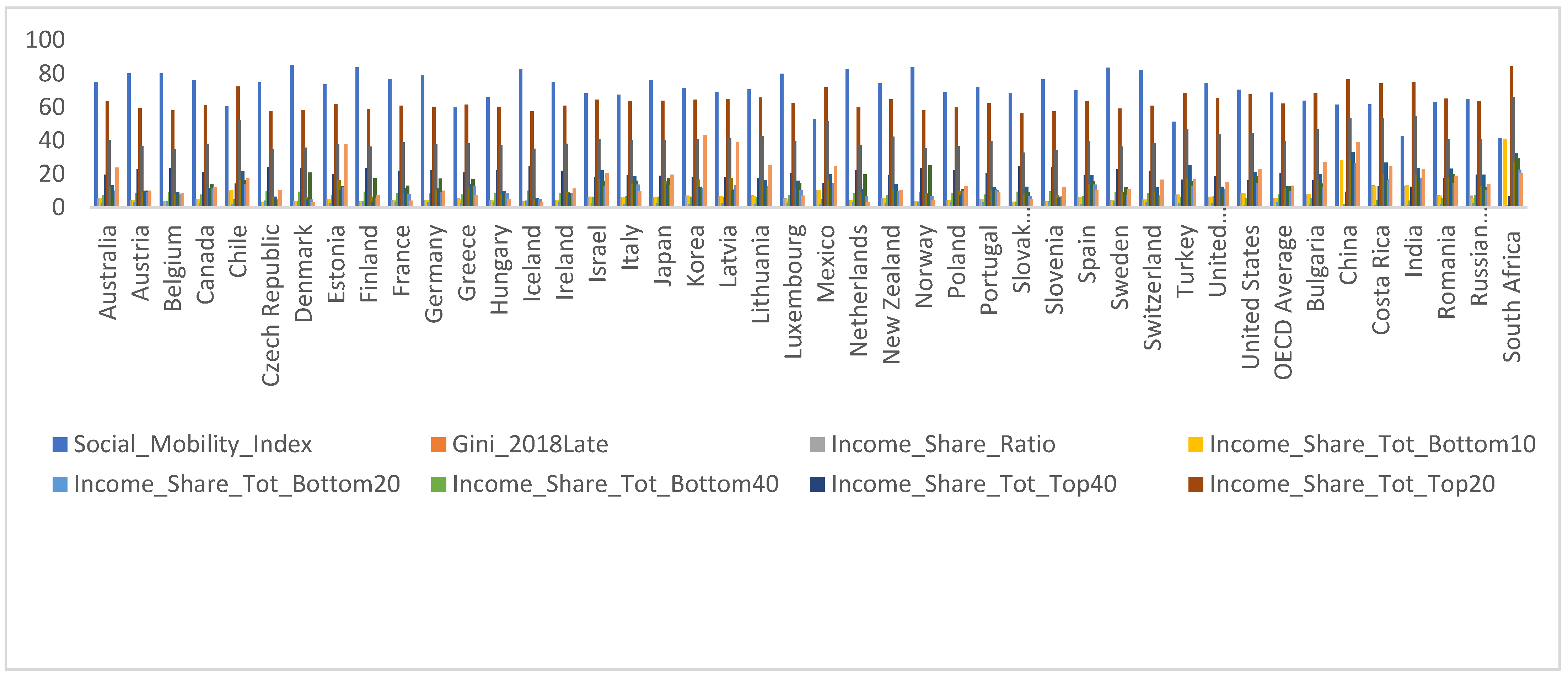Figure 2 below exhibits the sample of the countries used, as well as their corresponding data.

This Figure 2. Shows that most Nordic countries have the highest level of social mobility, followed by other high-income countries. However, Bulgaria, China, Costa Rico, India, Russia, and South Africa have the highest household poverty rates and income shares.

2. Methodology

The main objectives of this paper are: to estimate the transition probabilities of social mobility, to identify similar lower/higher mobility countries, and to analyze the impact of different types of inequality on intergenerational social mobility. To this end, the paper makes use of two statistical techniques, namely the Markov Switching process and the K-Means Cluster analysis.

2.1. Markov Switching Process

The transition probabilities of social mobility are computed from a Markov switching model regression model (Tong 1983; Hamilton 1989). This model can be specified as follows:

$$y_t=\{\begin{array}{c}{c}_1+{\displaystyle {\displaystyle \sum }_{i=1}^p}{\phi }_{i1}{x}_{it}+{\epsilon }_{1t};If{s}_t=1\\ c_2+{\displaystyle {\displaystyle \sum }_{i=1}^p}{\phi }_{i2}{x}_{it}+{\epsilon }_{2t}; If s_t=2\end{array}$$

(1)

where $s_t$ takes the value of 1 when a country is in a lower social mobility regime, and a value of 2 when it is in a higher social mobility regime. We assume that the mobility in each country is determined by the wealth inequality (Gini index), income ratio for the bottom 10, bottom 20, bottom 40, top 10, top 20, and top 40 households, and the level of poverty among children, youth, adult, elderly, and poor workers.

Hence, Equation (1) above is a first-order Markov chain with transition probabilities of switching between lower and higher social mobility regime and vice versa, given by:

Prob[s_t = 1 | s_t−1 = 1] = p₁₁
Prob[s_t = 2 | s_t−1 = 1] = 1 − p₁₁
Prob[s_t = 2 | s_t−1 = 2] = p₂₂
Prob[s_t = 1 | s_t−1 = 2] = 1 − p₂₂

(2)

The quantity $\frac{1}{p_{ii}}$ is refer to as the expected duration it takes a country to remain stagnant in one social mobility regime. $p_{ii}$ represents the sticky floors or sticky ceiling transition probabilities. Small values indicate that the duration of the stagnation period is longer than expected. The maximum likelihood method is used to estimate the parameters of the model in Equation (1).

2.2. K-Means Cluster Analysis

K-means is a clustering technique we use in this study to find groups of countries, such that the countries in one group have similar social mobility characteristics that are different (or unrelated) to those of the countries in other groups.

Given a set of macroeconomic variables such as the social mobility indices per country, income and poverty levels per country, the Gini coefficient indices per country, etc., we define a dataset $D$ made of data points $\left\{x_{1i}, x_{2i},\dots , x_{ni}\right\}$ representing the column of each macroeconomic variable in our sample of selected countries.

The K-means algorithm partitions the given dataset $D$ into k clusters each with its own center, called centroid. Given a desired number of clusters “K”, the K-means clustering technique/algorithm proceeds as follows:

• Randomly choose k data points to be the initial centroids;
• Assign each data point to the closest centroid;
• Re-compute the centroids using the current cluster memberships;
• If a convergence criterion is not met, no (or minimum) change of centroids, or minimum decrease in the sum of squared error—$SSE={\displaystyle \sum }_{j=1}^k{\displaystyle \sum }_{x\in C_j}dist{(x,m_j)}^2.$ where C_i is the jth cluster, m_j is the centroid of cluster C_j (the mean vector of all the data points in C_j), and dist(x, m_j) is the distance between data point x and centroid m_j.

3. Results

We developed a regression model with two hidden Markov processes: lower social mobility and higher social mobility. We assume that the social mobility of a country depends on its macroeconomic variables such as the income levels, poverty rates, and level of education.

Firstly, we use Equation (1) above to estimate the transition probabilities of individuals born to parents from the bottom half of the social ladder to make it to the top quartile of the social ladder. These probabilities are reported in

Table 1. Transition Probabilities of Social Mobilities.

	Bottom of the Social Ladder	Top of the Social Ladder
Bottom of the social Ladder	0.6726	0.4626
Top of the Social Ladder	0.3274	0.5374

Source: own calculation based on Markov Switching process.

below.

This table shows that, on average, there is a 67 percent chance that the children born to parents who were at the bottom of the social ladder will remain at the bottom quartile of their generation. Similarly, there is 54 percent chance that the children born to parents from the top quartile of the social ladder will remain at the top quartile of their generation. However, there is a 46 percent chance that children born to parents from the bottom of the social ladder will move to the top quartile of their generation, compared to only 33 percent for the children born to parents from the top to move downward to the bottom quartile of their generation.

These results emphasize the existence of a strong persistence in the top and bottom of the income distribution, implying that children born to parents from the top/bottom quartile remain at the top/bottom of the social ladder in their generation. These findings also suggest that there are high levels of income inequalities across all countries in our sample data. More importantly, these findings are consistent with those found in a 2018 OECD study that showed that there is a general trend toward more persistence of income positions at the bottom and at the top of the income distribution that translates into both lower chances to move to the top for those at the bottom of the social ladder, and lower chances to move downward for those at the top (Cingano 2014).

These findings are meaningless if we do not isolate countries with a similar lower/higher social mobility so that appropriate policy recommendations can be made at the national level. To achieve this, we make use of the K-means cluster analysis technique. This analysis is crucial in ascertaining whether income mobility is much lower in developing countries than in high-income countries. Figure 3 below exhibits the classification results using the K-means clustering. The x-axis represents the first principal component while the y-axis represents the second principal component of the social mobility dataset.

Figure 3 exhibits two types of social mobility categories—lower mobility countries highlighted in a light blue color include the United States, South Africa, China, Romania, Turkey, Bulgaria, Chile, Mexico, Costa Rico, and India. These countries have similar higher levels of inequalities (in income and access to wealth), suggesting that individuals born to parents from the top/bottom quartile in these countries tend to remain at the top/bottom quartile of their generation. The fact that the United States, a high-income country, is found to be in the same mobility category as developing countries such as South Africa and Mexico, is an astonishingly surprising finding. We argue that this might be due to internal socio-economic issues such as: low wages among low-skilled workers due to weak or non-existing labor unions, children born to rich parents have access to better schools and job opportunities, the lack of a universal healthcare system, etc. These results suggest that our hypothesis, that relative mobility is much lower in developing countries than in high-income countries, is not always true. Nevertheless, higher mobility countries highlighted in red include the Nordic countries, continental European countries, New Zealand, Canada, Korea, etc.

Impact of Inequalities on Social Mobility: Empirical Evidence

Lastly, we investigate the impact of inequalities (in income and wealth) based on the Great Gatsby Curve theory, which contends that countries with higher levels of inequalities tend to have lower levels of social mobility (Corak 2013a). We develop a Markov Switching regression model with two hidden Markov processes, namely the lower social mobility and the higher social mobility processes. We assume that the social mobility in each country is defined by the wealth inequality, income ratio for the bottom 10, bottom 20, bottom 40, top 10, top 20, and top 40 households, and the level of poverty among children, youth, adult, elderly, and poor worker.

Table 2. Estimated coefficients for the lower/higher mobility countries.

Panel I: Impact of inequalities on social mobility in lower mobility countries: Multiple R-squared: 0.9895.
Inequalities	Estimate	Std Error	T-Stat
Intercept	2732.44	6.511	419.665 ***
IncomeShareRatio	2.3686	0.2203	10.7517 ***
IncomSharTot_Bot10	7.3778	0.3409	21.6421 ***
IncomSharTot_Bot20	3.4207	4.0017	0.8548
IncomSharTot_Bot40	−28.036	4.8377	−5.7953 ***
IncomSharTot_Top40	−20.449	1.2174	−16.797 ***
IncomSharTot_Top20	−41.17	0.0902	−456.43 ***
IncomSharTot_Top10	9.4581	0.3914	24.1648 ***
PovertyRateChildren	11.7818	0.8495	13.8691 ***
PovertyRateYouth	−3.418	0.1863	−18.347 ***
PovertyRateAdult	−1.5957	0.1039	−15.358 ***
PovertyRateElderly	−12.883	0.6015	−21.418 ***
PovertyRateWorkpoor	−2.7526	0.1679	−16.394 ***
Gini2018Late	595.846	34.2245	17.4099 ***
Panel II: Impact of inequalities on social mobility in higher mobility countries: Multiple R-squared: 0.9964.
Inequalities	Estimate	Std Error	T-Stat
Intercept	−438.82	7.1312	−61.535 ***
IncomeShareRatio	−5.8239	0.2409	−24.176 ***
IncomSharTot_Bot10	−1.8391	0.1834	−10.028 ***
IncomSharTot_Bot20	−0.1448	3.3682	−0.043
IncomSharTot_Bot40	−6.5237	1.7793	−3.6664 ***
IncomSharTot_Top40	10.8575	0.295	36.8051 ***
IncomSharTot_Top20	5.9197	0.1224	48.3636 ***
IncomSharTot_Top10	−1.2999	0.2221	−5.8528 ***
PovertyRateChildren	6.5878	0.541	12.1771 ***
PovertyRateYouth	−1.7918	0.1393	−12.863 ***
PovertyRateAdult	−0.338	0.0586	−5.7679 ***
PovertyRateElderly	−3.2947	0.07	−47.067 ***
PovertyRateWorkpoor	−1.1897	0.1188	−10.014 ***
Gini2018Late	223.709	10.5812	21.1421 ***

Source: own calculation. Notes: ‘’***’’denote, the significance at 1% level.

below reports the estimated coefficients, the standard errors, and the test statistics. The significance at the 1 percent, 5 percent, and 10 percent level is shown with 3 stars, 2 stars, and 1 star, respectively.

Table 2 shows that generational earning elasticity has a positive relationship with inequality, as measured by the Gini coefficient, suggesting that in both lower and higher mobility countries, income inequality has a negative relationship with social mobility. These results are similar to the results of Corak (2013), who also found a positive relationship between generational earning elasticity and income inequality. Furthermore, poverty rates for all ages are found to be negatively correlated with the generational earning elasticity, suggesting that when poverty level decrease, intergenerational social mobility increases in both lower and higher mobility countries. The findings also show that the income of the bottom 10 and bottom 20 households is positively correlated with the generational earning elasticity in lower mobility countries and negatively correlated in the higher mobility countries. More studies are needed to identify the exact pattern of the relationship between the income of the bottom 40 and top 40 households and the generational earning elasticity in both lower and higher mobility countries.

Finally, we visualize the impact of each inequality type on the intergenerational social mobility plot and show how it affects cross-country discrepancies in relative mobility using the K-means clustering. Figure 4 below exhibits the relationship between inequality and intergenerational social mobility. We plot on the x-axis the global mobility index of each country, and on the y-axis, we plot the Gini coefficient index.

Figure 4 shows that the impact of income inequality, as measured by the Gini coefficient, is more pronounced in countries highlighted in a light blue color than in those highlighted in red. For example, India has the highest level of income inequality and the lowest level of intergenerational social mobility. Therefore, the impact of income inequality on intergenerational social mobility is more pronounced in India than in, for example, the Slovak Republic.

4. Conclusions

This paper is an empirical investigation into the impact of inequalities on intergenerational social mobility. The paper starts with the computation of transition probabilities that distinguish the likelihood that an individual born to parents from the bottom/top quartile will either move to the top/bottom or remain at the same quartile of her/his generation. To the best of our knowledge, this paper is the first to employ Markov Switching regression to compute these probabilities. It was found that there is a higher chance of stagnation in the top and bottom quartiles of the income/wealth distribution and that the likelihood of moving up or down the social ladder is minimal.

In addition, the paper identified two groups of countries with a similar lower/higher mobility. It was found that the hypothesis which stated that high-income countries have a higher relative social mobility does not always hold up in practice. The United States, a high-income country, was found to have a lower social mobility, similar to that of Turkey and South Africa.

Using a Markov Switching regression, this paper found that the poverty rates for all age group were negatively correlated with the generational earning elasticity, suggesting that when poverty decreases, intergenerational social mobility increases in both lower and higher mobility countries. Policies that promote the equality of opportunities at all stages of life are therefore recommended to improve the intergenerational social mobility. These policies might involve increasing public investment in early child education to prevent early school drops, increasing the healthcare support for children born to poor parents, and implementing a progressive tax system that provides more income support for disadvantaged families.