Multiclass Confusion Matrix Reduction Method and Its Application on Net Promoter Score Classification Problem

Abstract

The current paper presents a novel method for reducing a multiclass confusion matrix into a $2\times 2$ version enabling the exploitation of the relevant performance metrics and methods such as the receiver operating characteristic and area under the curve for the assessment of different classification algorithms. The reduction method is based on class grouping and leads to a special type of matrix called the reduced confusion matrix. The developed method is then exploited for the assessment of state of the art machine learning algorithms applied on the net promoter score classification problem in the field of customer experience analytics indicating the value of the proposed method in real world classification problems.

1. Introduction

1.1. Data Classification Problem Analysis

The problem of classification in the field of machine learning is an instance of pattern recognition [1]. The objective of the classification problem is to identify the class to which an observation belongs based on the set of associated features (explanatory variables). Typically, a set of training dataset of observations with known class membership is available, and in this context, classification is a special case of supervised learning. A classification problem can be further categorized into (a) binary classification problem in case that the class label can take only two values (e.g., A or B), (b) multiclass classification problem in case the class label can take more than two different values (e.g., A, B, C), and (d) multi-label classification problem in case that each observation is associated with multiple classes.

A wide variety of algorithms has been proposed for the solution of classification problems [1]. Example algorithms for binary classification include: linear regression, logistic regression, naïve Bayes, support vector machines, decision tree, random forest, k-nearest neighbors, convolutional neural networks, artificial neural networks, etc. It appears that depending on the specific problem type a different algorithm may be more appropriate. For that reason the performance of different algorithms should be evaluated before selecting the one that best fits the problem characteristics.

At the core of the performance evaluation of different classification algorithms we find the so called confusion matrix. The confusion matrix is defined as the matrix providing the mix of predicted vs. actual class instances. It allows for the definition of a wide range of performance metrics (e.g., accuracy, precision, recall, Mathews correlation coefficient, etc.) [2] or techniques such as the receiver operating characteristic (ROC) and area under the curve (AUC) [3]. In binary classification all performance metrics and ROC analysis are applicable. However, in multiclass classification only a limited set of performance metrics is available (typically accuracy, recall, precision, and F1-score). As mentioned in [3] ROC analysis is also applicable in multiclass classification problems, however, the complexity of analysis increases with the number of classes. Assuming a problem with N classes, a method for applying ROC analysis in this case is to derive a ROC chart for each class (considering the selected class as positive and the union of the rest classes as negative prediction) leading to N ROC charts. An analysis for a 3-dimensional classification problem is provided in [4].

The current paper provides a method which allows the application of the performance analysis available for a binary classification problem to a multiclass problem. The proposed method allows for the reduction in the dimension of a multiclass confusion matrix eventually reaching an equivalent form of a binary classification confusion matrix. The method is based on the ability to group the available class labels into sub-groups leading to a reduced confusion matrix which, as shown, has a specific structure depending on the way that classes are grouped. The paper then provides the formulation of the performance metrics for the reduced version of the confusion matrix and the way that ROC analysis can be performed. As a final step, the proposed method is applied to a specific multiclass classification problem associated with a customer experience metric (Net promoter score) indicating the method ability to support the algorithm performance evaluation in real world problems.

1.2. Customer Experience and Associated Metrics

Customer experience (CX) has been introduced as a concept a few decades ago [5,6,7,8,9] and since then it has evolved as a pillar of corporate strategy primarily aiming at customer loyalty and customer value. In this context, CX strategies are applied across industries and market sectors ranging from hotels, banks, retail stores, telecoms, and utility companies to health care, business to business, and e-commerce. Over time a set of best practices have been developed and shared across companies on how to build and implement CX strategies. Such practices include the introduction of CX programs with dedicated organizational roles, the inclusion of CX targets in the targets of all company units, the adoption of specific action plans with projects aiming at CX improvement, differentiation, and innovation.

The CX measurement framework is a key element of any CX program. Such a framework refers to a set of methods and metrics for measuring or characterizing the customer perceptions and the satisfaction level from the customer relation with a company. A number of CX metrics have been adopted for collecting customer feedback in an effective manner. Such metrics include net promoter score (NPS) [9], the customer satisfaction score (CSAT) [10] or the customer effort score (CES) [11]. These metrics are characterized by the question the customer is requested to respond to. In particular, the NPS question has the following form: “How likely is that you would recommend this company to your friends or colleagues?” The customer response in this case is an integer in a range from 0 to 10. Depending on the range of customer response customers are categorized as shown in

Table 1. The two most widely used customer categorizations.

(a) The NPS customer catergorization
NPS Response	NPS Label
9–10	Promoter
7–8	Passive
0–6	Detractor
(b) The CSAT customer catergorization
CSAT Response	CSAT Label
5	Very Satisfied
4	Satisfied
3	Neutral
2	Dissatisfied
1	Very Dissatisfied

a.

CSAT question has the following form: “How would you rate your overall satisfaction with this company?”. Customers may be requested to provide an integer score ranging from 1 to 5, 1 to 7, or 1 to 10 or select in multiple choice response ranging from “very dissatisfied” to “very satisfied”, as shown in Table 1b. CES question is in the form: “How easy was for you to complete this task or action?” with customers providing their response in the form of an integer ranging, e.g., from 1 to 10.

The measurement of CX metrics is performed based on two main methods:

• Market surveys: The survey is performed typically in a random sample of the market population. This method has the advantage of measuring CX for all market competitors. Moreover, apart from the main CX metric the survey also measures the customer satisfaction for a number CX attributes, such as the product experience, the value perception, the touchpoint experience (call center, website, mobile app, shops, etc.), or key customer journeys (e.g., billing, product purchase);
• Customer feedback during or right after a transaction: this method is used so as to measure the customer satisfaction at different stages of a transaction (or more generally a customer journey) or to measure the CX of a specific touchpoint (e.g., shop, call center, website, mobile app, etc.) Such measurements capture only the feedback of own customers, however, they can reveal significant customer insights.

Both methods are necessary for a successful CX program as they provide essential information on the direction that a company should follow in order to improve its competitive position in the market. The current paper focuses on the analysis applied on the market survey data. In particular, this analysis includes as a first step the monitoring of the CX metric and the CX attribute satisfaction trends vs. time and in comparison with the competing companies. The next step is the so called key drivers’ analysis which provides the link between CX attributes and the CX metric as described in the following section.

1.3. The CX Metric Classification Problem

The CX metric drivers’ analysis problem has the objective to identify the impact of the improvement of a CX attribute (e.g., website experience) to the overall CX Metric (e.g., NPS). This analysis allows companies to issue targeted actions of CX improvement with maximized impact on the overall CX metric. This problem is a multiclass classification problem as the CX metrics and the CX attribute satisfaction scores have integer scores within a specific range so they can be considered to be “labels”. The classification problem has the following formulation:

$$C\hat{X}M\left(i\right)=f(C{X}_{att}(i,1),C{X}_{att}(i,2),\dots ,C{X}_{att}(i,K))$$

(1)

where, $C\hat{X}M\left(i\right)$ is the CX metric score of survey responder i, $(i=1,2,\dots ,n)$, $C{X}_{att}(i,j)$, (j = 1, 2,…, K) is the satisfaction score of the same survey responder i, for CX attribute j and f is the function that allows for the association between these metrics.

The problem of CX metric classification can be addressed based on machine learning algorithms as shown in [12]. The confusion matrix of this problem is a multiclass confusion matrix with a dimension equal to the number of different class labels (i.e., the CX metric score labels). For example for NPS classification an $11\times 11$ confusion matrix will occur (class labels: 0, 1, 2,…,10) and for CSAT classification a $5\times 5$, $7\times 7$, or $10\times 10$ confusion matrix will occur depending on the score range applied in the relevant questionnaire (1–5, 1–7, 1–10, accordingly). The following section provides an overview of the state of the art regarding the way that the performance of the various algorithms applied for solving a multiclass classification problem.

2. Classification Algorithm Performance Analysis

As mentioned in the introduction, there is a set of performance metrics which can be applied on the confusion matrix of a classification problem so as to assess an algorithm or compare the performance of different algorithms. The confusion matrix for a binary and a multiclass classification problem are presented in Figure 1a,b accordingly. Each column of the matrix represents the instances of a predicted class, while each row represents the instances of an actual class. An element of the confusion matrix at row i and column j provides the number of instances for which the predicted class is j and the actual class is i. In this context, the confusion matrix shows the ways in which the classification model is “confused” when it makes predictions. It can provide the insight not only into the errors being made by a classifier, but more importantly the type of the resulting errors.

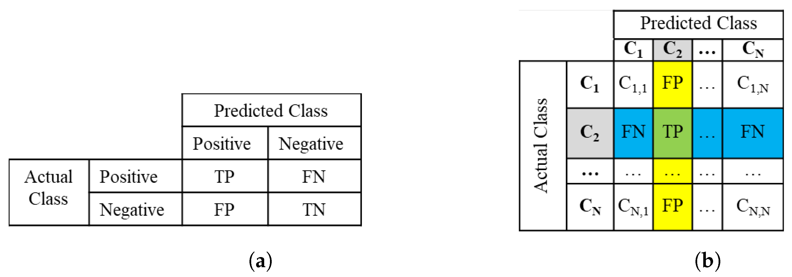
2.1. Algorithm Performance for Binary Classification Problems

In the case of a binary classification problem, the confusion matrix has a dimension of $2\times 2$ (Figure 1a) where one of the labels is considered to be “Positive” and the other one “Negative”. The matrix elements are characterized based on the predicted label (positive, negative) and the result of the comparison of the predicted with the actual class label (true, false) [13]: true positives (TP), true negatives (TN), false positives (FP), and false negatives (FN). A wide number of performance metrics have been defined for the binary classification confusion matrix as shown in

Table 2. The performance metrics of the binary classification confusion matrix.

Metric	Formula
Accuracy	$Acc={\displaystyle \frac{TP+TN}{TP+TN+FP+FN}}$
True Positive Rate (Recall)	$TPR={\displaystyle \frac{TP}{TP+FN}}$
True Negative Rate (Specificity)	$TNR={\displaystyle \frac{TN}{TN+FP}}$
Positive Predictive Value (Precision)	$PPV={\displaystyle \frac{TP}{TP+FP}}$
Negative Predictive Value	$NPV={\displaystyle \frac{TN}{TN+FN}}$
$F_1$-Score	$F_1=2·{\displaystyle \frac{TPR·PPV}{TPR+PPV}}$
False Negative Rate (Miss Rate)	$FNR={\displaystyle \frac{FN}{TP+FN}}$
False Positive Rate (Fall Out Rate)	$FPR={\displaystyle \frac{FP}{TN+FP}}$
False Discovery Rate	$FDR={\displaystyle \frac{FP}{TP+FP}}$
False Omission Rate	$FOR={\displaystyle \frac{FN}{TN+FN}}$
Fowlkes-Mallows index	$FM=\sqrt{PPV·TPR}$
Balanced Accuracy	$BA={\displaystyle \frac{TPR+TNR}{2}}$
Mathews Correlation coefficient	$MCC={\displaystyle \frac{TP·TN-FP·FN}{\sqrt{(TP+FN)(TP+FP)(FN+TN)(FP+TN)}}}$
Prevalence Threshold	$PT={\displaystyle \frac{\sqrt{TPR(1-TNR)}+TNR-1}{TPR+TNR-1}}$
Informedness	$BM=TPR-FPR$
Markedness	$MK=PPV-FOR$
Threat Score (Critical Success Index)	$TS={\displaystyle \frac{TP}{TP+FN+FP}}$

[14,15].

In principle, not a single metric can judge the performance of an algorithm and for that reason multiple metrics should be taken into account. Moreover, when data instances are imbalanced (e.g., the number of negative instances is substantially lower vs. the positive instances) some metrics may provide a misleading picture.

An advanced method for assessing the performance of a binary classification algorithm is the so called receiver operating characteristic (ROC) [3]. This is a methodology which provides a chart of true positive rate or recall (TPR) vs. false positive rate or fall out rate (FPR). The resulting chart corresponds to the metrics occurring when a specific threshold $\theta$ ranging from 0 to 1 is applied as a criterion for selecting the positive or the negative Prediction based on the probabilities assigned to the positive and negative states as an outcome of the algorithm. The ROC chart allows to compare the performance of an algorithm with the random selection algorithm (an algorithm that selects the positive or the negative class randomly), as well as with the performance of another algorithm. In the ROC space (i.e., pairs of TPR, FPR) the random selection algorithm is characterized by the straight line connecting the points (0,0) and (1,1). Any algorithm performing better than the random selection algorithm should have its ROC curve points lying above this straight line and vice versa.

The area under the curve (AUC) is a metric defined in a ROC chart as the area under the ROC curve of an algorithm. Hence, the higher the AUC value the better the algorithm performance. The AUC (combined with the observation of the ROC curve) allows for the comparison of different algorithms by selecting the algorithms with the highest AUC metric as the best performing ones.

2.2. Multiclass Confusion Matrix and Metrics

In the case of multiclass classification, the metrics defined for binary classification, do not apply in full extend. The multiclass confusion matrix (see Figure 1b) has a dimension N × N where N is the number of different class labels $C_0,C_1,\dots ,C_N$ (e.g., 11 for NPS). Therefore the characterization of TP, TN, FP, FN instances is not applicable in this case. Instead, it is feasible to perform an analysis focusing on a specific class based on the characterization provided in the example of Figure 1b. A set of metrics for each class can be defined based on this approach. Then, based on the proper combination of these metrics it is feasible to provide metrics for the entire confusion matrix.

Table 3. Performance metrics for a multiclass confusion matrix.

Metric	Formula
Accuracy	$Acc\left(A_{reduced}\right)={\displaystyle \frac{{\sum }_{i=1}^{N}TP\left(C_i\right)}{{\sum }_{i=1}^N{\sum }_{j=1}^N{C}_{i,j}}}$
Recall of Class $C_i$	$TPR\left(C_i\right)={\displaystyle \frac{TP\left(C_i\right)}{TP\left(C_i\right)+FN\left(C_i\right)}}$
Precision of Class $C_i$	$PPV\left(C_i\right)={\displaystyle \frac{TP\left(C_i\right)}{TP\left(C_i\right)+FP\left(C_i\right)}}$
$F_1$-Score of Class $C_i$	$F_1\left(C_1\right)=2·{\displaystyle \frac{TPR\left(C_i\right)·PPV\left(C_i\right)}{TPR\left(C_i\right)·PPV\left(C_i\right)}}$
Recall (macro average)	$TPR\left(macro\right)={\displaystyle \frac{1}{N}}{\sum }_{i=1}^{N}TPR\left(C_i\right)$
Precision (macro average)	$PPV\left(macro\right)={\displaystyle \frac{1}{N}}{\sum }_{i=1}^{N}PPV\left(C_i\right)$
$F_1$-Score (macro average)	$F_1\left(macro\right)=2·{\displaystyle \frac{TPR\left(macro\right)·PPV\left(macro\right)}{TPR\left(macro\right)+PPV\left(macro\right)}}$
Recall (micro average)	$TPR\left(micro\right)={\displaystyle \frac{{\sum }_{i=1}^{N}TP\left(C_i\right)}{{\sum }_{i=1}^N[TP\left(C_i\right)+FP\left(C_i\right)]}}$
Precision (micro average)	$PPV\left(micro\right)={\displaystyle \frac{{\sum }_{i=1}^{N}RP\left(C_i\right)}{{\sum }_{i=1}^N[TP\left(C_i\right)+FP\left(C_i\right)]}}$
$F_1$-Score (micro average)	$F_1\left(micro\right)=2·{\displaystyle \frac{TPR\left(micro\right)·PPV\left(micro\right)}{TPR\left(micro\right)+PPV\left(micro\right)}}$

provides an overview of the metrics defined for a multiclass confusion matrix and, in particular, accuracy, recall, precision, and $F_1$-score. As it can be seen there are two main approaches in defining performance metrics called “micro” and “macro”.

3. Multiclass Confusion Matrix Reduction Methods

Let us consider a multiclass classification problem with set A containing the N different class labels $C_i(i=1,2,\dots ,N)$ of the dependent parameter of the problem: $A=\{C_1,C_2,\dots ,C_N\}$. The confusion matrix for that problem is an $N\times N$ matrix with the form of Figure 1b. The concept of the reduction process of such a multiclass confusion matrix originates from the fact that often from the problem analysis viewpoint, classes could be grouped into sets of classes. For example, in the problem of NPS or CSAT classification, customers with a certain score range can be assigned to specific categories (e.g., NPS between 0 and 6 are categorized as “detractors”, as shown in Table 1a).

Since the class labels can be re-ordered without affecting the resulting performance metrics of a multiclass confusion matrix, without loss of generality we may consider a group of classes as a sub-set of the set of classes defined as follows:

$$G=\{C_1,C_2,\dots ,C_m\},G\subset A$$

(2)

An example of such a grouping of classes is presented in Figure 2. As shown in this figure there is a clear definition of false positives (FP) and false negatives (FN) instances. False positives correspond to instances for which the predicted class belongs to Grouped class G and the actual class does not belong to group G. Vice versa, false negatives correspond to instances for which the predicted class does not belong to group G while the actual class belongs to group G. Regarding true positives (TP) there are some options analyzed in the following section. The total FP and FN instances of the group G are provided as follows:

$$FP\left(G\right)=\sum _{C_i\notin G}\sum _{C_j\in G}{C}_{i,j},FN\left(G\right)=\sum _{C_i\in G}\sum _{C_j\notin G}{C}_{i,j}$$

(3)

3.1. Class Grouping Options

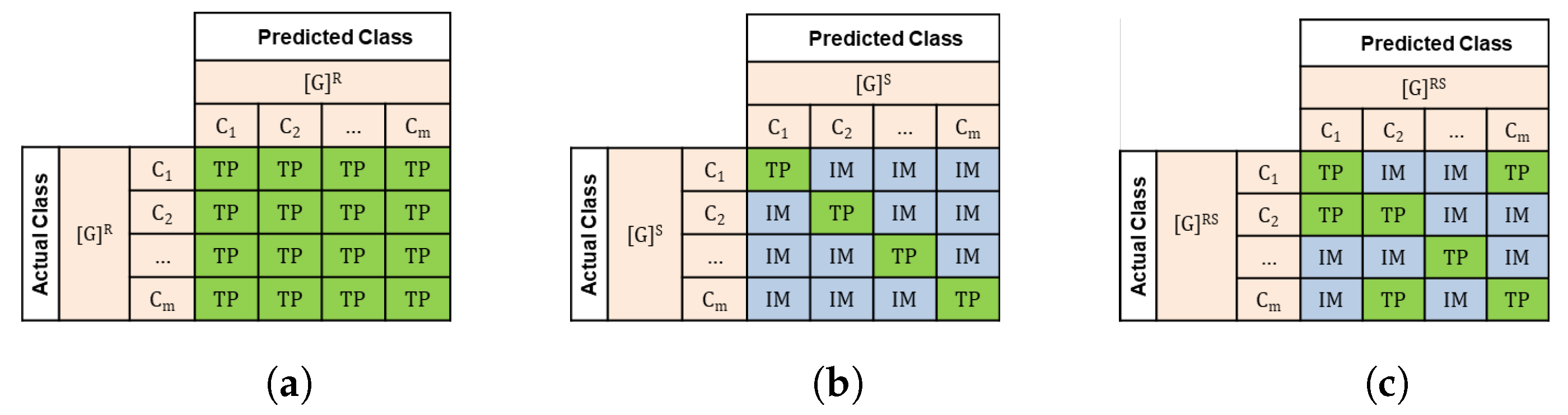
Regarding the definition of TP for group G the following three options were identified and presented in Figure 3:

• Relaxed Grouping of Classes${\left[G\right]}^R$: As shown in Figure 3a, in this case any prediction of a class $C_i\in G$ with actual class $C_j\in G$ is considered to be a true positive instance. In the example of NPS classification, assuming that we are interested in the group of detractors (score from 0 to 6) then a prediction of score 1 with an actual score 3 is considered to be true positive since both the predicted and the actual group is “detractor”;
• Strict Grouping of Classes${\left[G\right]}^S$: As shown in Figure 3b, in this case only the predictions $C_i\in G$ which are identical to the actual class are considered to be true positive instances, i.e., only the instances $C_{i,i}$ with $C_i\in G$. For example, assuming the grouped class of detractors in NPS problem, if the predicted class is 3 then a TP instance occurs only if the actual class is 3;
• Hybrid-RS Grouping of Classes${\left[G\right]}^{RS}$: As shown in Figure 3c, in this case apart from the instances where the predicted class is identical to the actual class, there is an additional set of combinations of predicted and actual classes which are considered to be a TP instance. For example, assuming the group of detractors in NPS problem, assume that we are interested in an algorithm that predicts the scores that are equal of better than the actual scores.

The selection of the proper class grouping option is subject to the nature and the requirements of the specific classification problem under study.

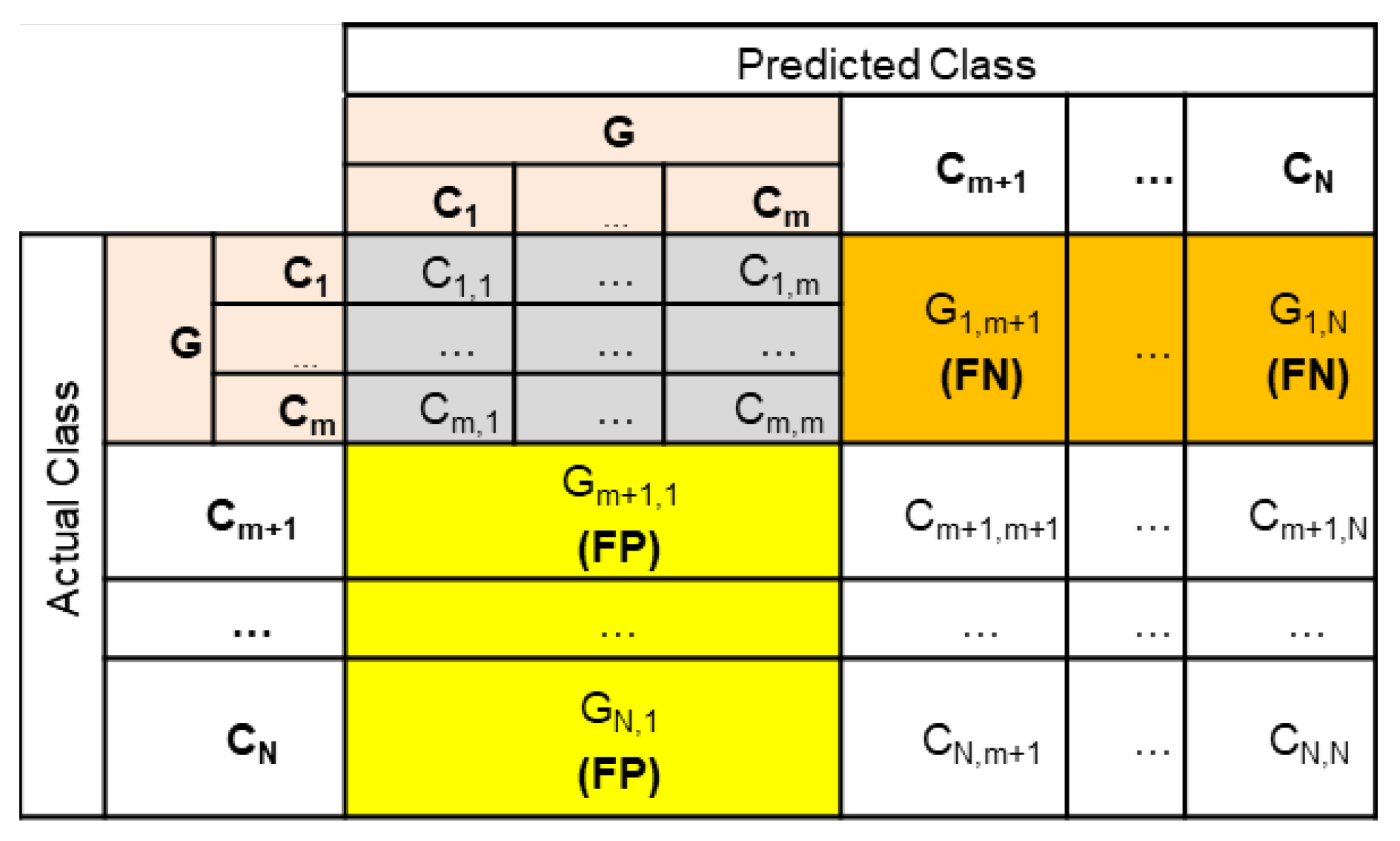
3.2. The Grouped Class Formal Definition

Based on the above class grouping options we define the “Grouped Class” as a pair of two sets as follows:

$${\left[G\right]}^H=(G,G_{TP}(G,H))$$

(4)

where, G is the subset of A containing the classes that are grouped as defined in Equation (2). H indicates the applied grouping option with the following values: (a) R (for Relaxed), (b) S (for Strict) and (c) $RS$ (for Hybrid-RS). $G_{TP}$ is defined as the set of True Positive combinations for this specific grouping as follows:

$$G_{TP}(G,H)=\{(C_i,C_j):C_i,C_j\in G\mathrm{and}G\mathrm{is}\mathrm{a}\mathrm{TP}\mathrm{instance}\mathrm{based}\mathrm{on}H\mathrm{option}\}$$

(5)

In this case, the number of TP instances for any grouping scheme is the following:

$$TP({\left[G\right]}^H)=\sum _{(C_i,C_j)\in G_{TP(G,H)}}{C}_{i,j}$$

(6)

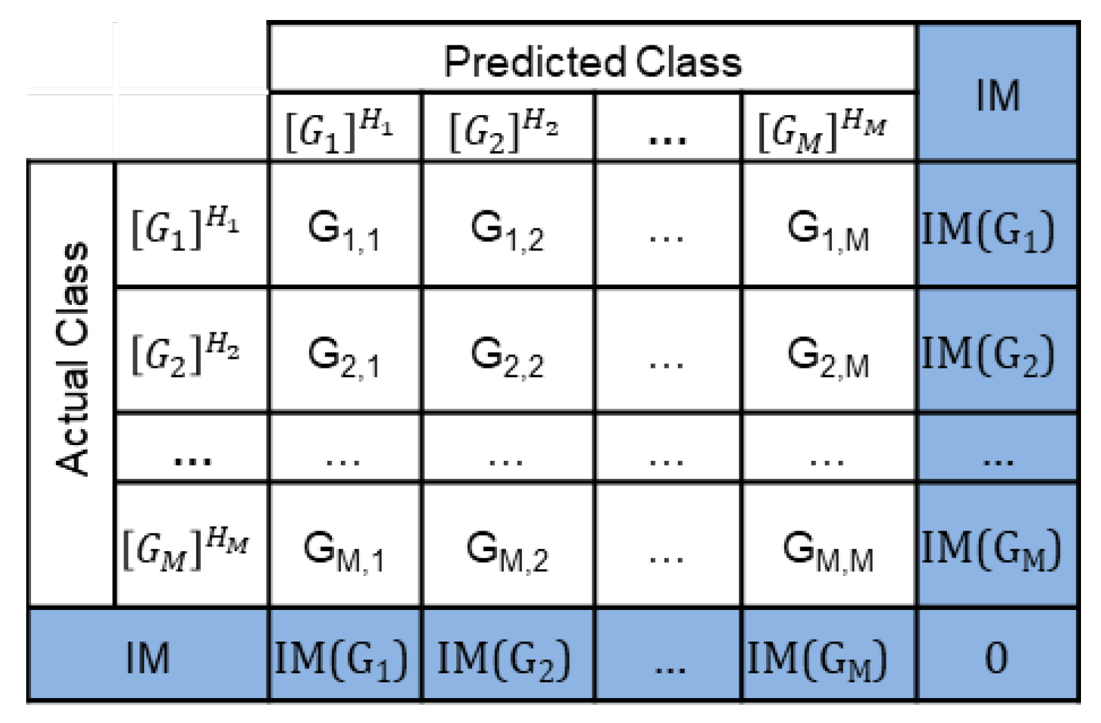
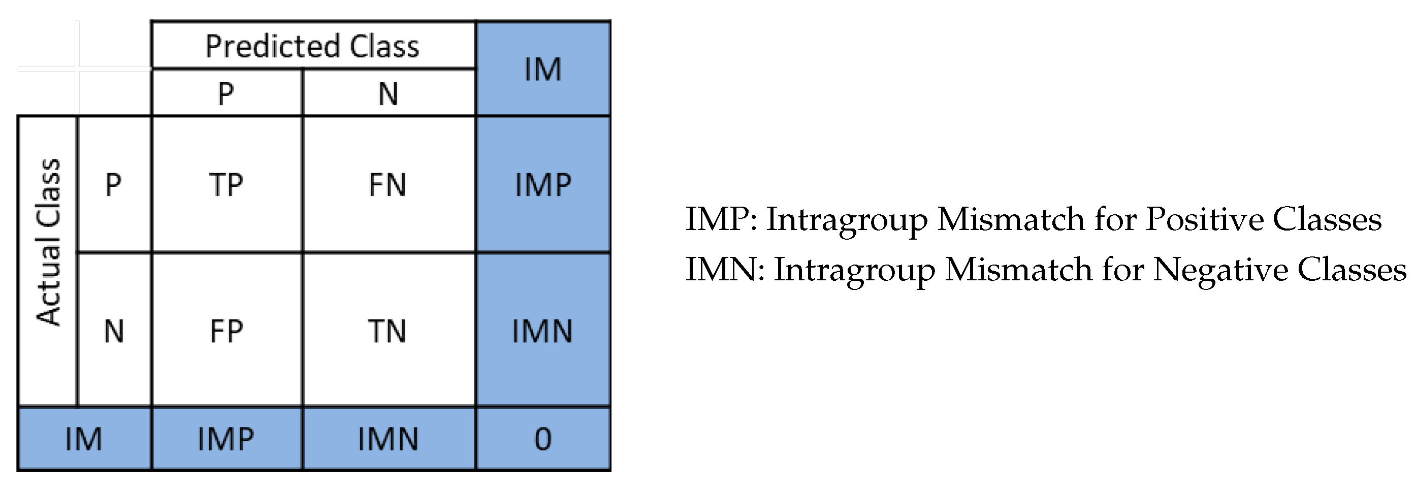
3.3. The Intragroup Mismatch Instances

As also observed from Figure 3, in the case of strict and hybrid-RS grouping there is a set of instances which cannot be characterized as TP. These instances are called intragroup mismatch (IM) instances because both the predicted and the actual class belong to the same group G (thus, intragroup) however, the predicted class is different than the actual one and do not correspond to a TP instance (i.e., a mismatch). According to the definition of $G_{TP}$ set they can be calculated as follows $(H=R,S,RS)$:

$$IM({\left[G\right]}^H)=\sum _{C_i,C_j\in G,(C_i,C_j)\notin G_{TP(G,H)}}{C}_{i,j}$$

(7)

From Equations (6) and (7) we achieve:

$$TP({\left[G\right]}^H)+IM({\left[G\right]}^H)=\sum _{C_i,C_j\in G}{C}_{i,j}$$

(8)

As a consequence of these definitions, the total number of predicted instances that belongs to G and the total number of actual instances that belong to G will be $(H:R,S,RS)$:

$$n_{predicted}({\left[G\right]}^H)=TP({\left[G\right]}^H)+FP({\left[G\right]}^H)+IM({\left[G\right]}^H)$$

(9)

$$n_{actual}({\left[G\right]}^H)=TP({\left[G\right]}^H)+FN({\left[G\right]}^H)+IM({\left[G\right]}^H)$$

(10)

The above equations indicate clearly that IM of group G cannot be considered to be either FP or FN. The way that IM instances are treated is covered in the following section.

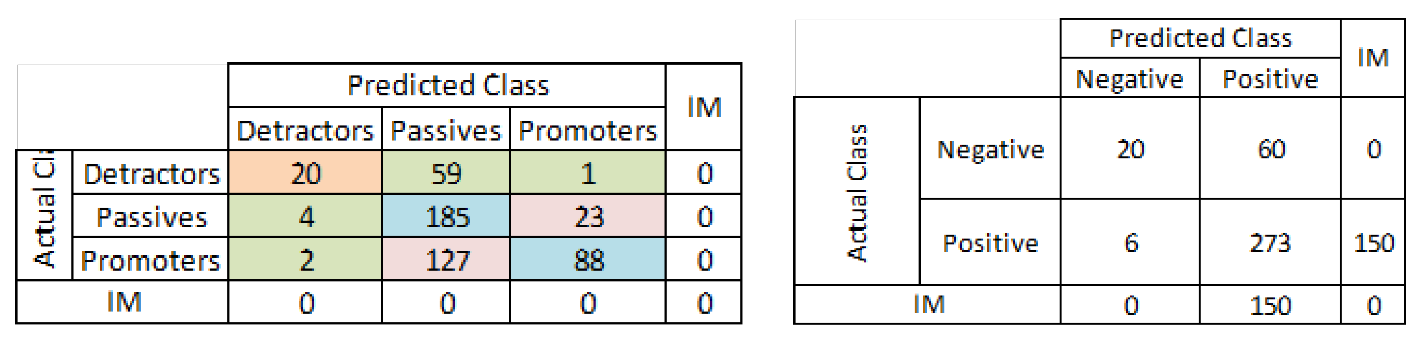
4. The Concept of the Reduced Confusion Matrix

Based on the definitions of the previous section, it is now possible to define a grouping of classes of the original multiclass confusion matrix as a number of M grouped classes. To achieve this, the original set of classes A is split into a number of M disjoint subsets (groups) with the following properties:

$$G_j\subset A,j=1,2,\dots ,M,\mathrm{for}i\ne j,G_i\cap G_j=\varnothing \mathrm{and}{\cup }_{i=1}^M{G}_i=A$$

(11)

Then, for each subset of classes G_j a grouping option H_j is being selected $(R,S,RS)$ leading to a set of grouped classes G_A defined as follows:

$$G_A=\{{\left[G_1\right]}^{H_1},{\left[G_2\right]}^{H_2}.\dots ,{\left[G_M\right]}^{H_M},H_j=R,SorRS\}$$

(12)

Based on the above definition of the set of grouped classes we can now define the reduced confusion matrix shown in Figure 4. The representation of the reduced version of the confusion matrix should also take into account the new category of intragroup mismatch (IM) instances. To achieve this, we consider a specific format for the reduced confusion matrix called “$M\times M+IM$” (M indicates the new reduced dimension of the confusion matrix and $IM$ indicates the presence of intragroup mismatch instances), as presented in the example of Figure 4. In this new proposed format the $IM$ category is introduced as an extra row and column with the column being the transposed version of the $IM$ row. This matrix format leads to Equations (9) and (10) when summing up the instances in column or the row of group G_j so as to calculate the number of actual or the number of predicted instances accordingly.

4.1. Consecutive Confusion Matrix Reduction Steps

Based on the rationale developed in the previous section, it is now possible to define a multi-step confusion matrix reduction process where in the general case either classes or the original matrix or groups of classes can further be grouped according to the problem specific requirements. Based on Equations (11) and (12) the set of grouped classes of step k can be defined as follows:

$$G_A\left(k\right)=\left\{{\left[G_{k,1}\right]}^{H_{k,1}},{\left[G_{k,2}\right]}^{H_{k,2}},\dots ,{\left[G_{k,M_k}\right]}^{H_{k,M_k}}\right\}$$

(13)

$$G_{k,i}\subset G_A(k-1),i=1,2,\dots ,M_k$$

(14)

$$\mathrm{For}i\ne j,G_{k,i}\cap G_{k,j}=\varnothing \mathrm{and}\bigcup _{i=1}^{M_k}{G}_{k,i}=G_A(k-1)$$

(15)

$$G_A\left(0\right)=A,G_{0,i}=C_i,H_{0,i}=R,i=1,2,\dots ,M$$

(16)

where, $G_A\left(k\right)$ is set of grouped classes at step $k(k\ge 0)$, $M_k$ is the number of grouped classes ($M_k\ge 2$), $G_{k,i},i=1,2,\dots ,M_k$ is the $i\mathrm{th}$ grouped class of step k, $H_{k,i}$ is the applied grouping option (R, S or RS) for the $i\mathrm{th}$ grouped class of step $k\left(G_{k,i}\right)$. Equation (16) provides the initial conditions of the process, i.e., the link to the original set of problem classes A.

In each step of this process, the confusion matrix of the previous step is considered as the basis. According to this approach, the number of FP, FN, TP, and IM instances for a specific grouped class ${\left[G_{k,M_k}\right]}^{H_{k,M_k}}$ can be derived from the generalization of the Equations (3), (7) and (8) as follows:

$$FP\left({\left[G_{k,M_k}\right]}^{H_{k,M_k}}\right)=\sum _{G_{k-1,i}\notin G_{k,m}}\sum _{G_{k-1,j}\in G_{k,m}}{G}_{k-1,i,j}$$

(17)

$$FN\left({\left[G_{k,M_k}\right]}^{H_{k,M_k}}\right)=\sum _{G_{k-1,i}\in G_{k,m}}\sum _{G_{k-1,j}\notin G_{k,m}}{G}_{k-1,i,j}$$

(18)

$$TP\left({\left[G_{k,M_k}\right]}^{H_{k,M_k}}\right)=\sum _{(G_{k-1,i},G_{k-1,j})\notin G_{TP}(G_{k,m},H_{k,m})}{G}_{k-1,i,j}$$

(19)

$$IM\left({\left[G_{k,M_k}\right]}^{H_{k,M_k}}\right)=\sum _{G_{k-1,i}\in G_{k,m}}IM\left(G_{k-1,i}\right)+\sum _{G_{k-1,i},G_{k-1,j}\in G_{k,m},G_{k-1,i,j}\in G_{TP}(G_{k,m},H_{k,m})}{G}_{k-1,i,j}$$

(20)

where, $G_{k-1,i,j}$ is the number of instances where the actual class belongs to grouped class $G_{k-1,i}$ and the predicted class belongs to grouped class $G_{k-1,j}$.

It is easy to show that when the applied grouping option in a consecutive reduction process is either relaxed (R) or strict (S) then the following property applies:

$${\left[{\cup }_j,{\left[G_j\right]}^H\right]}^H={\left[{\cup }_{c_i\in \left[{\cup }_j{G}_j\right]},\left\{C_i\right\}\right]}^H,\mathrm{for}H\mathrm{either}R\mathrm{or}S$$

(21)

In the case that different grouping methods are applied in each step then the above property does not hold.

4.2. Performance Metrics for a Reduced Confusion Matrix

The performance metrics for an “$M\times M+IM$” reduced confusion matrix ($M>2$) are defined according to the formulas of

Table 4. Performance metrics of reduced confusion matrix.

Metric	Formula
Accuracy of Reduced Confusion Matrix	$Acc\left(A_{reduced}\right)={\displaystyle \frac{{\sum }_{j}TP\left({\left[G_j\right]}^{H_j}\right)}{{\sum }_{j}TP\left({\left[G_j\right]}^{H_j}\right)+{\sum }_i{\sum }_{j,i\ne j}{G}_{i,j}+{\sum }_{j}IM\left({\left[G_j\right]}^{H_j}\right)}}$
Recall of Group $G_j$	$TPR\left({\left[G_j\right]}^{H_j}\right)={\displaystyle \frac{TP\left({\left[G_j\right]}^{H_j}\right)}{TP\left({\left[G_j\right]}^{H_j}\right)+FN\left({\left[G_j\right]}^{H_j}\right)+IM\left({\left[G_j\right]}^{H_j}\right)}}$
Precision of Group $G_j$	$PPV\left({\left[G_j\right]}^{H_j}\right)={\displaystyle \frac{TP\left({\left[G_j\right]}^{H_j}\right)}{TP\left({\left[G_j\right]}^{H_j}\right)+FP\left({\left[G_j\right]}^{H_j}\right)+IM\left({\left[G_j\right]}^{H_j}\right)}}$

. Based on the calculation of recall and precision metrics for a specific group of classes, as shown in Table 4, it is feasible to estimate the reduced confusion matrix metrics based on macro average and micro average according to the formulas of Table 3.

Moreover, it is very easy to show that for the same set of classes G, the following properties apply regarding the applied grouping options:

$$TP({\left[G\right]}^S)\le TP({\left[G\right]}^H),H=R,S,RS$$

(22)

$$Acc({\left[G\right]}^S)\le Acc({\left[G\right]}^H),H=R,S,RS$$

(23)

It is also easy to observe that when strict grouping is applied the accuracy of the reduced confusion matrix equals to the accuracy of original confusion matrix.

In the case that the confusion matrix reduction process leads to a “$2\times 2+IM$” confusion matrix, then the confusion matrix has the form of Figure 5.

In this case the typical binary classification confusion matrix metrics can be also calculated based on the following observation regarding the number of positive and negative instances:

$$\mathrm{Actual}\mathrm{Positives}:P_{actual}=TP+FN+IMP$$

(24)

$$\mathrm{Predicted}\mathrm{Positives}:P_{predicted}=TP+FP+IMP$$

(25)

$$\mathrm{Actual}\mathrm{Negatives}:N_{actual}=TN+FP+IMN$$

(26)

$$\mathrm{Actual}\mathrm{Negatives}:N_{predicted}=TN+FN+IMP$$

(27)

The performance metrics presented in Table 2 for a $2\times 2$ confusion matrix have been properly adapted for the “$2\times 2+IM$” confusion matrix and presented in

Table 5. Performance metrics of reduced confusion matrix.

Metric	Formula
Accuracy	$Acc={\displaystyle \frac{TP+TN}{TP+TN+FP+FN+IMP+IMN}}$
True Positive Rate (Recall)	${\displaystyle \frac{TP}{(TP+FN+IMP)}}$
True Negative Rate (Specificity)	${\displaystyle \frac{TN}{TN+FP+IMN}}$
Positive Predictive Value (Precision)	$PPV={\displaystyle \frac{TP}{TP+FP+IMP}}$
Negative Predictive Value	$NPV={\displaystyle \frac{TN}{TN+FN+IMN}}$
False Negative Rate (Miss Rate)	$FNR={\displaystyle \frac{FN}{TP+FN+IMP}}$
False Positive Rate (Fall Out Rate)	$FPR={\displaystyle \frac{FP}{TN+FP+IMN}}$
False Discovery Rate	$FDR={\displaystyle \frac{FP}{TP+FP+IMP}}$
False Omission Rate	$FOR={\displaystyle \frac{FN}{TN+FN+IMN}}$

. Note, that the formulas of Table 2 still apply for the metrics (using, however, the revised version of the required input parameters as provided in Table 5): $F_1$-score, Fowlkes–Mallows index, balanced accuracy, prevalence threshold, informedness, markedness, and threat score (critical success index).

The Mathews correlation coefficient based on the proof provided in Appendix A is provided by the following equation:

$$MCC={\displaystyle \frac{IMP·IMN+(TP+IMP)TN-FN·FP}{\sqrt{(TP+FN+IMP)(TP+FP+IMP)(FN+TN+IMN)(FP+TN+IMN)}}}$$

(28)

Moreover, we define the following new metrics related to intragroup mismatch rates:

$$\mathrm{Positive}\mathrm{IM}\mathrm{Rate}:PIMR={\displaystyle \frac{IMP}{TP+FN+IMP}}$$

(29)

$$\mathrm{Negative}\mathrm{IM}\mathrm{Rate}:NIMR={\displaystyle \frac{IMN}{TN+FP+IMN}}$$

(30)

$$\mathrm{Positive}\mathrm{Predictive}\mathrm{IM}\mathrm{Rate}:PPIMR={\displaystyle \frac{IMP}{TP+FP+IMP}}$$

(31)

$$\mathrm{Negative}\mathrm{Predictive}\mathrm{IM}\mathrm{Rate}:NPIMR={\displaystyle \frac{IMN}{TN+FN+IMN}}$$

(32)

Based on the above definitions (Equation (29) to Equation (32)) we achieve:

$$TPR+PIMR+FNR=1$$

(33)

$$TNR+NIMR+FPR=1$$

(34)

$$PPV+PPIMR+FDR=1$$

(35)

$$NPV+NPIMR+FOR=1$$

(36)

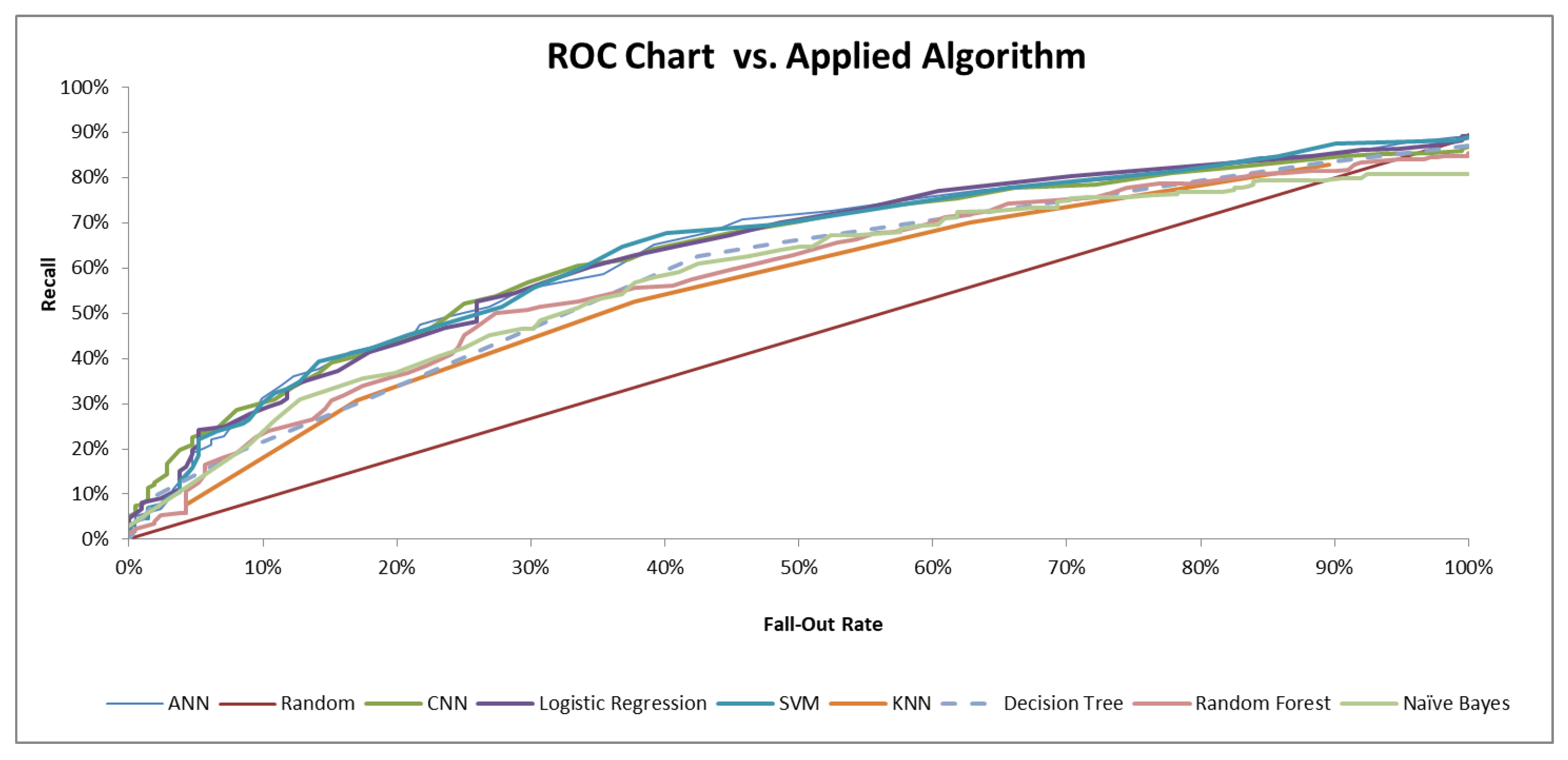
4.3. Receiver Operating Characteristic for a Reduced $2\times 2+IM$ Confusion Matrix

Since ROC chart and the related metric of AUC is a commonly used method to assess the performance of different classification algorithms, it would be advantageous to define a method to derive ROC chart and AUC metric for a reduced $2\times 2+IM$ confusion matrix.

A two-step approach is followed in this case for the identification of the predicted class:

• Step 1: As in the ordinary binary classification, the prediction of positive vs. negative grouped class is based on a threshold $\theta$;
• Step 2: The prediction of a specific class from the set of grouped positive or negative classes is based on maximum likelihood.

Based on this approach the ROC chart can be derived based on precision (TPR) and fall-out rate (FPR) metrics based on the equations provided in Table 5. In particular, as the threshold approaches zero ($\theta \to 0$) all predictions will be negatives. So we obtain:

$$\underset{\theta \to 0}{lim}TP=0,\underset{\theta \to 0}{lim}FP=0,\underset{\theta \to 0}{lim}IMP=0$$

(37)

$$\underset{\theta \to 0}{lim}TN=T{N}_{ML},\underset{\theta \to 0}{lim}FN=P_{actual},\underset{\theta \to 0}{lim}IMN=N_{actual}-T{N}_{ML}$$

(38)

$$\underset{\theta \to 0}{lim}TPR=0,\underset{\theta \to 0}{lim}FPR=0$$

(39)

where, $N_{actual}$ is the number of actually negative instances, $P_{actual}$ is the number of actual positive instances and $T{N}_{ML}$ is the number of true negative instances based on maximum likelihood selection of the predicted class as $\theta$ approaches 0.

When the threshold approaches one ($\theta \to 1$) all predictions will be positives. So we obtain:

$$\underset{\theta \to 1}{lim}TP=T{P}_{ML},\underset{\theta \to 1}{lim}FP=N_{actual},\underset{\theta \to 1}{lim}IMP=P_{actual}-T{P}_{ML}$$

(40)

$$\underset{\theta \to 1}{lim}TN=0,\underset{\theta \to 1}{lim}FN=0,\underset{\theta \to 1}{lim}IMN=0$$

(41)

$$\underset{\theta \to 1}{lim}TPR=T{P}_{ML}/P_{actual},\underset{\theta \to 1}{lim}FPR=1$$

(42)

where $P_{actual}$ is the number of actually positive instances and $T{P}_{ML}$ is the number of true positive instances based on maximum likelihood selection of the predicted class when $\theta$ approaches 1.

Based on the above analysis, it appears that the ROC space for a reduced confusion matrix is the following: $TPR$ in $[0,T{P}_{ML}/P_{actual}]$ and $FPR$ in $[0,1]$. This range is the same for all the applied algorithms. However, the ratio $T{P}_{ML}/P_{actual}$ may depend on the applied algorithm. Moreover, it is very easy to show that the random selection process corresponds to the straight line between the points: $(0,0)$ and $(T{P}_{ML}/P_{actual},1)$.

The area under the curve (AUC) can be estimated based on the following definition [14]:

$$AUC={\int }_0^{1}TPR\left(FP{R}^{-1}\left(\theta \right)\right)d\theta$$

(43)

5. Confusion Matrix Reduction for NPS Classification

In this section, we apply the proposed method to the NPS classification problem for a grouping scenario based on specific business requirements.

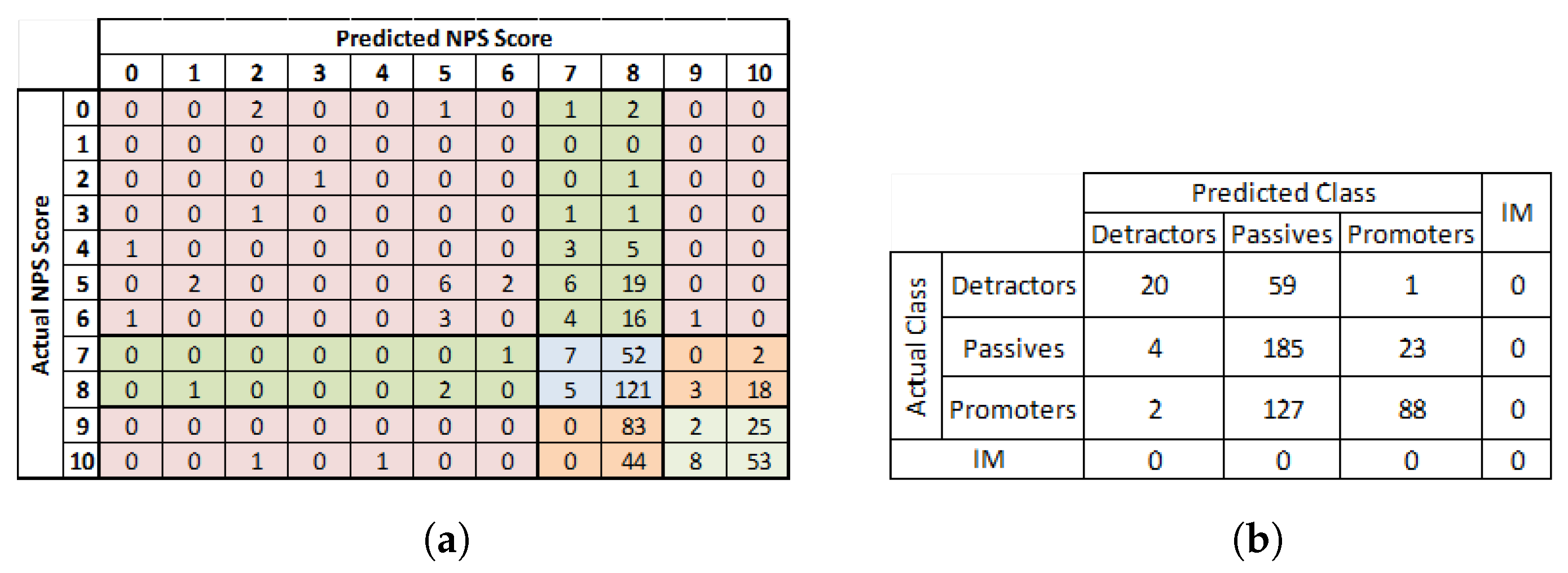
5.1. NPS Classification Dataset

The analysis has been performed using real NPS survey data from the Greek mobile communication market. The dataset corresponds to a set of approximately 2500 samples per operator collected in a period of 6 consecutive months based on market surveys. For confidentiality purposes the set of data used for the analysis presented in this paper correspond to random selection of approximately 2500 responses from customers of the three different operators.

Each NPS survey was based on a questionnaire which apart from the NPS question it also included questions on the customer level of satisfaction from a set of 9 customer experience attributes: tariff plan, network voice service, network data service, shops, call center, website, mobile application, billing, and roaming service.

5.2. Machine Learning Algorithms for NPS Classification

The NPS classification problem can then be formulated as shown in Equation (1). In our NPS survey data analysis, the NPS classification problem refers to the consideration of the customer scores on the 9 customer experience attributes as a basis to predict the NPS score of each individual responder. Such an analysis allows for the identification of the level of contribution or the importance of each one of the 9 attributes in the formulation of the NPS score.

In this paper, the following algorithms have been tested for the NPS classification problem [12]: logistics regression (LR), k-nearest neighbor (k-NN), naïve Bayes (NB), support vector machines (SVM), decision trees (DT), random forest (RF), convolutional neural networks (CNN), and artificial neural networks (ANN).

The available NPS survey data of approximately 2500 samples were split into training and validation data with an 80–20% ratio. Further details on the applied algorithms are provided in Appendix B.

5.3. Confusion Matrix for the NPS Classification Problem

The original set of classes in this case corresponds to the 11 different classes of NPS score (0–10):

$$A\left(NPS\right)=\left\{0,1,2,3,4,5,6,7,8,9,10\right\}$$

(44)

The NPS classification problem has an $11\times 11$ confusion matrix, as shown in Figure 6a resulting from the application of logistic regression algorithm to the NPS survey data. Based on the definition of the confusion matrix reduction process the following grouping steps can be applied:

Step 1: Relaxed grouping based on the definition of customer categories: detractor, passive and promoter (as shown in Figure 6a):

$$\begin{array}{cc}\hfill A_{reduced}\left(NPS\right)& =\left\{{[0,1,2,3,4,5,6]}^R,{[7,8]}^R,{[9,10]}^R\right\}\hfill \\ \hfill & =\left\{C_{detractors},C_{passives},C_{promoters}\right\}\hfill \end{array}$$

(45)

The above reduced confusion matrices has the form of $3\times 3+IM$, as shown in Figure 6. Note that since the applied grouping is relaxed (R) all $IM$ values are zero.

Step 2: In order to compare the performance of different classification algorithms we are going to consider the following grouping step:

$$A_{reduced}^{\prime }\left(NPS\right)=\{{\left[C_{detractors}\right]}^S,{[C_{passives},C_{pormoters}]}^S\}$$

(46)

In the reduced set of classes, a customer may belong to one of the two available grouped classes depending on the NPS score: (a) detractor (considered to be the negative case) and (b) either a promoter or a passive (considered to be the positive case).

The result of this step is a reduced confusion in the form of $2\times 2+IM$ (see Figure 7) which allows the extensive performance analysis of different classification algorithms.

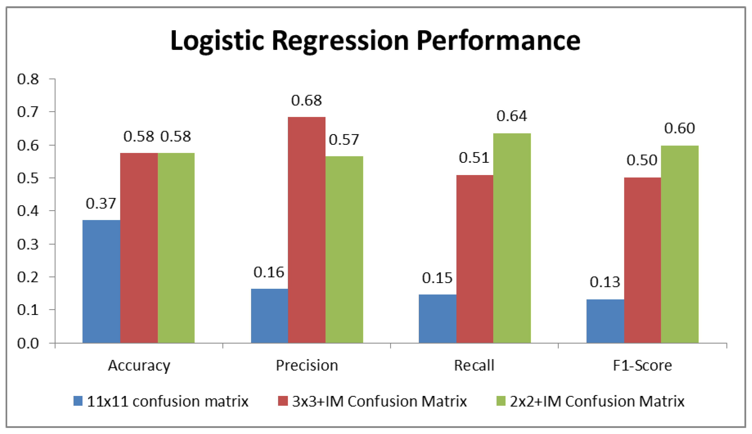
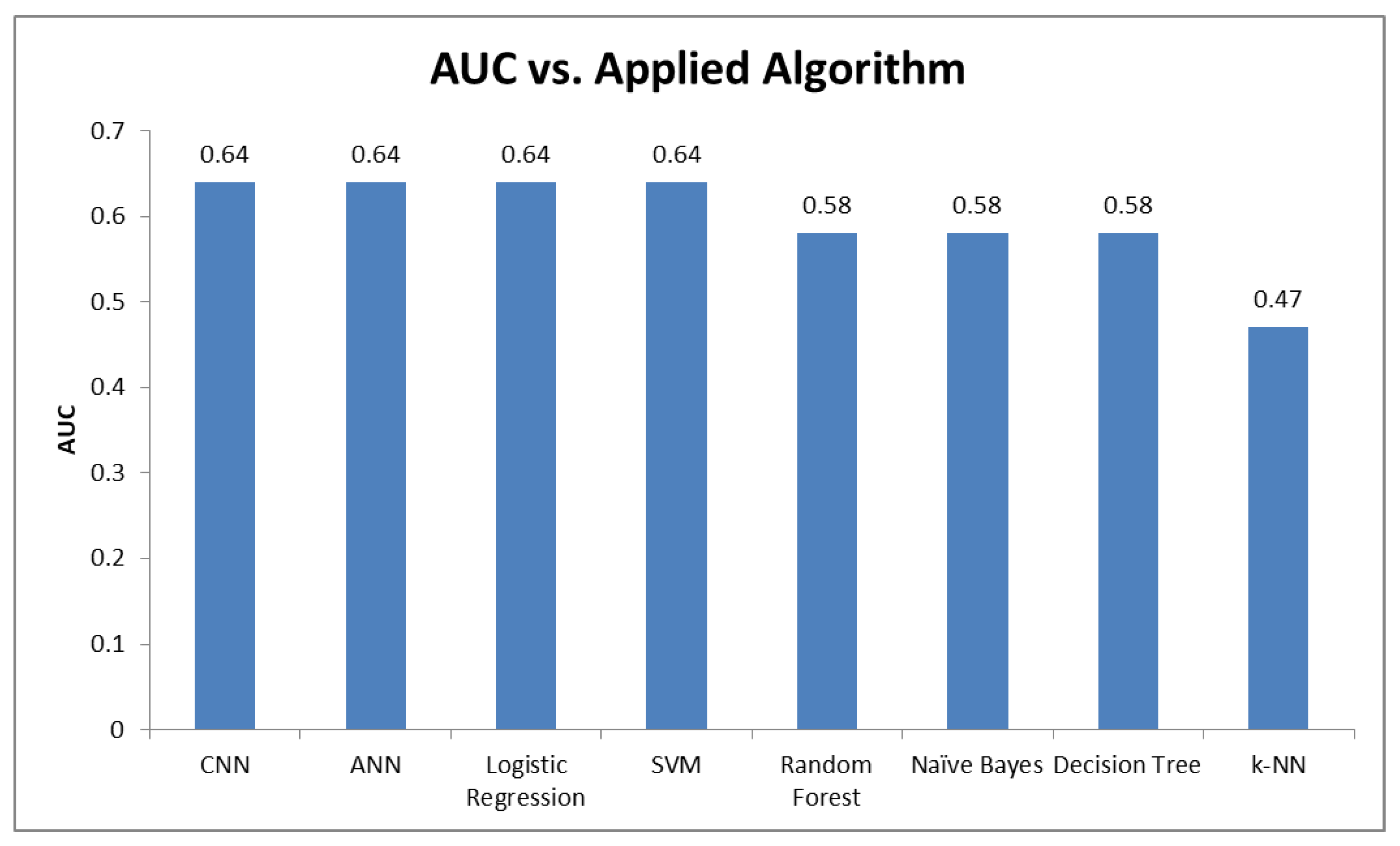
5.4. Performance Results

The analysis presented above has been followed for all the machine learning algorithms listed in Section 5.2. Just like in the example of logistic regression presented in Figure 6 and Figure 7, every machine learning algorithm led to the production of an original $11\times 11$ confusion matrix which was then reduced according to the steps presented in the previous section into a $3\times 3+IM$ and then into a $2\times 2+IM$ reduced confusion matrix.

The following tables provide the performance metrics derived for each tested machine learning algorithm. Specifically,

Table 6. The performance metrics of the $11\times 11$ confusion matrix for each applied algorithm.

	Logistic Regr.	SVM	k-NN	Decision Trees	Random Forest	Naïve Bayes	CNN	ANN
Accuracy	0.37	0.38	0.34	0.39	0.33	0.31	0.38	0.37
Precision	0.16	0.17	0.17	0.23	0.19	0.17	0.21	0.14
Recall	0.15	0.17	0.16	0.22	0.17	0.15	0.19	0.17
F1-score	0.13	0.14	0.16	0.21	0.18	0.15	0.19	0.15

provides the performance metrics for the original $11\times 11$ confusion matrix,

Table 7. The performance metrics of the “$3\times 3+IM$” reduced confusion matrix for each applied algorithm.

	Logistic Regr.	SVM	k-NN	Decision Trees	Random Forest	Naïve Bayes	CNN	ANN
Accuracy	0.58	0.56	0.60	0.51	0.54	0.56	0.63	0.57
Precision	0.68	0.65	0.62	0.50	0.55	0.54	0.66	0.69
Recall	0.51	0.48	0.56	0.50	0.50	0.58	0.60	0.52
F1-score	0.50	0.53	0.58	0.50	0.51	0.57	0.62	0.51

provides the metrics for the reduced $3\times 3+IM$ confusion matrix, and

Table 8. The performance metrics of the “$2\times 2+IM$” reduced confusion matrix for each one of the applied algorithms.

	Logistic Regr.	SVM	k-NN	Decision Trees	Random Forest	Naïve Bayes	CNN	ANN
Accuracy	0.58	0.56	0.60	0.51	0.54	0.56	0.63	0.57
Precision	0.57	0.55	0.60	0.52	0.54	0.62	0.62	0.56
Recall	0.64	0.61	0.63	0.52	0.58	0.54	0.65	0.62
F1-Score	0.60	0.58	0.61	0.52	0.56	0.58	0.63	0.59
Specificity	0.09	0.07	0.16	0.15	0.11	0.27	0.19	0.10
Miss Rate	0.01	0.01	0.05	0.10	0.05	0.19	0.04	0.02
Negative Predictive Value	0.11	0.09	0.18	0.15	0.13	0.21	0.21	0.13
Fall Out Rate	0.14	0.10	0.10	0.10	0.12	0.06	0.09	0.13
False Discovery Rate	0.12	0.10	0.10	0.10	0.12	0.07	0.09	0.12
False Omission Rate	0.03	0.01	0.11	0.18	0.11	0.32	0.08	0.04
Fowlkes-Mallows index	0.60	0.58	0.61	0.52	0.56	0.58	0.63	0.59
Mathews Correlation Coefficient	0.33	0.37	0.35	0.37	0.36	0.34	0.38	0.36
PIMR	0.35	0.39	0.32	0.38	0.37	0.27	0.31	0.36
PPIMR	0.31	0.35	0.30	0.38	0.35	0.31	0.30	0.32

provides the results for the reduced $2\times 2+IM$ confusion matrix.

The first issue considered is the impact of the confusion matrix reduction steps on the performance metrics. Figure 8 compares the metrics of 11 × 11, $3\times 3+IM$ and $2\times 2+IM$ confusion matrices of the NPS classification problem based on logistic regression. This figure indicates a substantial improvement of the metrics when relaxed grouping is applied (from $11\times 11$ to $3\times 3+IM$ reduction). This is expected as in relaxed grouping the cases considered to be true positive increases compared to the original confusion matrix. This can be observed in the example of Figure 6a,b. In the second grouping step (from $3\times 3+IM$ to $2\times 2+IM$ reduction) the application of strict grouping leads to the same accuracy while differences of smaller scale are observed in the rest metrics (precision, recall, $F_1$-score). This is also explained by the fact that in strict grouping the number of true positives remains the same so accuracy metric is not affected (this can be also derived from Equations (22) and (23)).

The second issue considered is the ability to compare the performance of machine learning algorithms for the same classification problem (i.e., NPS classification). As it can be seen from Table 6 where the metrics for the $11\times 11$ confusion matrix are provided, decision trees appear to outperform the rest of the algorithms for all available metrics (accuracy, precision, recall, and $F_1$-score). However, the actual level of these metrics is rather low (e.g., accuracy 0.39). This analysis compares the algorithms in their ability to correctly predict the NPS score (i.e., from 0 to 10). Considering the results of the $3\times 3+IM$ reduced confusion matrix in Table 7 we observe that CNN algorithm outperforms the rest algorithms in accuracy, recall, and $F_1$-score metrics while considering precision metric ANN algorithm outperforms CNN. These results indicate that CNN is probably the most appropriate algorithm in predicting the customer NPS class, i.e., detractor, passive, promoter with an accuracy level of 0.63. Regarding the results of the $2\times 2+IM$ reduced confusion matrix presented in Table 8, we observe that CNN algorithm outperforms the rest algorithms for the majority of the available metrics. The table indicates the ability to deep dive in the comparison of algorithms with the availability of metrics such as the Mathews correlation coefficient. Moreover, metrics such as PIMP and PPIMP indicate the performance of the algorithm in terms of the resulting portion of cases under Intra-group mismatch category.

To complete the comparison of the performance of the applied algorithms we may apply ROC analysis for the $2\times 2+IM$ matrix of each algorithm. Figure 9 provides the ROC charts of the $2\times 2+IM$ matrix and Figure 10 provides the relevant AUC values. The ROC analysis leads to the conclusion that the best performing algorithms are CNN, ANN, logistic regression, and SVM which clearly outperform the rest of the algorithms. The figures demonstrate the value of the proposed method in assessing the performance of the applied machine learning algorithms.

6. Conclusions

The paper deals with the performance analysis of multi-class classification algorithms based on the analysis of the associated multi-class confusion matrix. Triggered from the fact that the available performance metrics for a multi-class confusion matrix are limited compared to a binary classification problem, the current paper proposes a method that reduces the dimensions of a multi-class confusion matrix based on class grouping process. The key method outcomes include: (a) the options of class grouping (relaxed, strict, and hybrid RS grouping) which are selected based on the classification problem requirements (b) the definition of the “reduced confusion matrix” with an extra row and a column for the intragroup mismatch (IM) instances (c) the performance metrics formulas for a reduced confusion matrix and (d) the application of ROC, AUC analysis for a reduced $2\times 2+IM$ confusion matrix.

The paper has applied the proposed method in the case of NPS classification problem demonstrating the capability of the method to handle an $11\times 11$ confusion matrix. Based on the NPS classification problem specific characteristics, a two-step grouping approach was followed allowing for the performance analysis of a wide range of machine learning algorithms. The results of ROC analysis indicate that CNN, ANN, logistic regression, and SVM outperform random forest, naïve Bayes, decision trees, and k-NN algorithms for this specific problem. Based on these results and taking into account that NPS scoring patterns may change dynamically depending on the market conditions the next research steps include the investigation of techniques that can further improve the performance of neural networks such as the ones proposed in [16] (retraining of neural networks) and [17] (deep learning framework applied to dynamically changing conditions).

The proposed method can be applied to any multiclass classification problem since the applied classification algorithms always lead to the generation of multiclass confusion matrix. As shown with the example of NPS classification, to exploit the proposed method, the appropriate grouping of classes should be applied depending on the problem specific characteristics and the scope of the analysis. A topic for future research will be the investigation of potential generic grouping approaches that would allow the analysis of multiclass classification problems for which the grouping of classes may not be an obvious task (e.g., optical character recognition, animal species classification, etc.).

References

1. Alpaydin, E. Introduction to Machine Learning; The MIT Press: Cambridge, MA, USA, 2020. [Google Scholar]
2. Matthews, B.W. Comparison of the Predicted and Observed Secondary Structure of T4 Phage Lysozyme. Biochim. Biophys. Acta-(Bba)-Protein Struct. 1975, 405, 442–451. [Google Scholar] [CrossRef]
3. Fawcett, T. An Introduction to ROC Analysis. Pattern Recognit. Lett. 2006, 27, 861–874. [Google Scholar] [CrossRef]
4. Mossman, D. Three-Way ROCs. Med Decis. Mak. 1999, 19, 78–89. [Google Scholar] [CrossRef]
5. Bolton, R.N.; Drew, J.H. A Multistage Model of Customers’ Assessments of Service Quality and Value. J. Consum. Res. 1991, 17, 375–384. [Google Scholar] [CrossRef]
6. Aksoy, L.; Buoye, A.; Aksoy, P.; Larivière, B.; Keiningham, T.L. A Cross-National Investigation of the Satisfaction and Loyalty Linkage for Mobile Telecommunications Services across Eight Countries. J. Interact. Mark. 2013, 27, 74–82. [Google Scholar] [CrossRef]
7. Rageh Ismail, A.; Melewar, T.C.; Lim, L.; Woodside, A. Customer Experiences with Brands: Literature Review and Research Directions. Mark. Rev. 2011, 11, 205–225. [Google Scholar] [CrossRef] [Green Version]
8. Gentile, C.; Spiller, N.; Noci, G. How to Sustain the Customer Experience:: An Overview of Experience Components That Co-Create Value With the Customer. Eur. Manag. J. 2007, 25, 395–410. [Google Scholar]
9. Reichheld, F.F.; Covey, S.R. The Ultimate Question: Driving Good Profits and True Growth; Harvard Business School Press: Boston, MA, USA, 2006; Volume 211. [Google Scholar]
10. Fornell, C.; Johnson, M.D.; Anderson, E.W.; Cha, J.; Bryant, B.E. The American Customer Satisfaction Index: Nature, Purpose, and Findings. J. Mark. 1996, 60, 7–18. [Google Scholar] [CrossRef] [Green Version]
11. de Haan, E.; Verhoef, P.C.; Wiesel, T. The Predictive Ability of Different Customer Feedback Metrics for Retention. Int. J. Res. Mark. 2015, 32, 195–206. [Google Scholar] [CrossRef]
12. Markoulidakis, I.; Rallis, I.; Georgoulas, I.; Kopsiaftis, G.; Doulamis, A.; Doulamis, N. A Machine Learning Based Classification Method for Customer Experience Survey Analysis. Technologies 2020, 8, 76. [Google Scholar] [CrossRef]
13. Stehman, S.V. Selecting and Interpreting Measures of Thematic Classification Accuracy. Remote. Sens. Environ. 1997, 62, 77–89. [Google Scholar] [CrossRef]
14. Powers, D. Evaluation: From Precision, Recall and F-Measure to ROC, Informedness, Markedness & Correlation. arXiv 2020, arXiv:2010.16061. [Google Scholar]
15. Tharwat, A. Classification Assessment Methods. Appl. Comput. Inform. 2020. [Google Scholar] [CrossRef]
16. Doulamis, A.; Doulamis, N.; Kollias, S. On-Line Retrainable Neural Networks: Improving the Performance of Neural Networks in Image Analysis Problems. IEEE Trans. Neural Netw. 2020, 11, 137–155. [Google Scholar] [CrossRef]
17. Doulamis, N.; Voulodimos, A. FAST-MDL: Fast Adaptive Supervised Training of Multi-Layered Deep Learning Models for Consistent Object Tracking and Classification. In Proceedings of the 2016 IEEE International Conference on Imaging Systems and Techniques (IST), Chania, Greece, 4–6 October 2016; pp. 318–323. [Google Scholar] [CrossRef]
18. Quinlan, J.R. Induction of Decision Trees. Mach. Learn. 1986, 1, 81–106. [Google Scholar] [CrossRef] [Green Version]
19. Rokach, L.; Maimon, O.Z. Data Mining with Decision Trees: Theory and Applications; World Scientific: Singapore, 2007. [Google Scholar]
20. Bhatia, N. Survey of nearest neighbor techniques. arXiv 2010, arXiv:1007.0085. [Google Scholar]
21. Murphy, K.P. Machine Learning: A Probabilistic Perspective; MIT Press: Cambridge, MA, USA, 2012. [Google Scholar]
22. Protopapadakis, E.; Voulodimos, A.; Doulamis, A.; Camarinopoulos, S.; Doulamis, N.; Miaoulis, G. Dance Pose Identification from Motion Capture Data: A Comparison of Classifiers. Technologies 2018, 6, 31. [Google Scholar] [CrossRef] [Green Version]
23. Keller, J.M.; Gray, M.R.; Givens, J.A. A Fuzzy K-Nearest Neighbor Algorithm. IEEE Trans. Syst. Man Cybern. 1985, 580–585. [Google Scholar] [CrossRef]
24. Abe, S. Support Vector Machines for Pattern Classification; Advances in Pattern Recognition; Springer: London, UK, 2010. [Google Scholar] [CrossRef]
25. Smola, A.J.; Schölkopf, B. A Tutorial on Support Vector Regression. Stat. Comput. 2004, 14, 199–222. [Google Scholar] [CrossRef] [Green Version]
26. Kopsiaftis, G.; Protopapadakis, E.; Voulodimos, A.; Doulamis, N.; Mantoglou, A. Gaussian Process Regression Tuned by Bayesian Optimization for Seawater Intrusion Prediction. Comput. Intell. Neurosci. 2019, 2019, e2859429. [Google Scholar] [CrossRef]
27. Pal, M. Random Forest Classifier for Remote Sensing Classification. Int. J. Remote Sens. 2005, 26, 217–222. [Google Scholar] [CrossRef]
28. Haykin, S.; Network, N. A comprehensive foundation. Neural Netw. 2004, 2, 41. [Google Scholar]
29. Hecht-Nielsen, R.; Drive, O.; Diego, S. Kolmogorov’s Mapping Neural Network Existence Theorem. In Proceedings of the International Conference on Neural Networks; IEEE Press: New York, NY, USA, 1987; Volume 3, pp. 11–14. [Google Scholar]
30. Doulamis, N.; Doulamis, A.; Varvarigou, T. Adaptable Neural Networks for Modeling Recursive Non-Linear Systems. In Proceedings of the 2002 14th International Conference on Digital Signal Processing Proceedings. DSP 2002 (Cat. No.02TH8628), Santorini, Greece, 1–3 July 2002; Volume 2, pp. 1191–1194. [Google Scholar] [CrossRef]
31. Voulodimos, A.; Doulamis, N.; Doulamis, A.; Protopapadakis, E. Deep Learning for Computer Vision: A Brief Review. Comput. Intell. Neurosci. 2018, 2018, 1–13. [Google Scholar] [CrossRef]
32. Protopapadakis, E.; Voulodimos, A.; Doulamis, A. On the Impact of Labeled Sample Selection in Semisupervised Learning for Complex Visual Recognition Tasks. Complexity 2018, 2018, e6531203. [Google Scholar] [CrossRef]
33. Doulamis, A.; Doulamis, N.; Protopapadakis, E.; Voulodimos, A. Combined Convolutional Neural Networks and Fuzzy Spectral Clustering for Real Time Crack Detection in Tunnels. In Proceedings of the 2018 25th IEEE International Conference on Image Processing (ICIP), Athens, Greece, 7–10 October 2018; pp. 4153–4157. [Google Scholar] [CrossRef]
34. Haouari, B.; Ben Amor, N.; Elouedi, Z.; Mellouli, K. Naïve Possibilistic Network Classifiers. Fuzzy Sets Syst. 2009, 160, 3224–3238. [Google Scholar] [CrossRef]
35. Hosmer, D.W.; Lemeshow, S. Applied Logistic Regression; John Wiley & Sons: New York, NY, USA, 2000. [Google Scholar]
Figure 1. Confusion matrix examples. (a) Binary classification problem confusion matrix. (b) Multiclass classification problem confusion matrix.
Technologies 09 00081 g001
Figure 2. Confusion matrix class grouping example.
Technologies 09 00081 g002
Figure 3. True positive instances definition examples. (a) TP for relaxed grouping. (b) TP for strict grouping. (c) Example TP for hybrid RS-grouping.
Technologies 09 00081 g003
Figure 4. The reduced confusion matrix “ M × M + I M ” format ( H = R , S , R S ).
Technologies 09 00081 g004
Figure 5. The concept of reduced confusion matrix in “ 2 × 2 + I M ” form.
Technologies 09 00081 g005
Figure 6. The reduction in the 11 × 11 NPS classification confusion matrix into a 3 × 3 + I M reduced confusion matrix. (a) The 11 × 11 NPS confusion matrix. (b) The reduced 3 × 3 + I M confusion matrix.
Technologies 09 00081 g006
Figure 7. The reduction in the 3 × 3 + I M confusion matrix into a 2 × 2 + I M .
Technologies 09 00081 g007
Figure 8. Logistic regression performance for the original and reduced confusion matrices.
Technologies 09 00081 g008
Figure 9. The ROC chart for NPS classification problem.
Technologies 09 00081 g009
Figure 10. The AUC vs. the applied algorithm.
Technologies 09 00081 g010