An EWMA-DiD Control Chart to Capture Small Shifts in the Process Average Using Auxiliary Information


Abstract
:1. Introduction
2. Designing of EWMA-DiD Control Chart
3. Performance of the Proposed EWMA-DiD Control Chart
| Algorithm 1. Monte Carlo Simulation Program of EWMA-DiD Control Chart for in-control and shifted process |
The following are the algorithmic steps involved in Monte Carlo Simulation R program.
|
4. Comparison of EWMA-DiD Control Chart with Other Control Charts
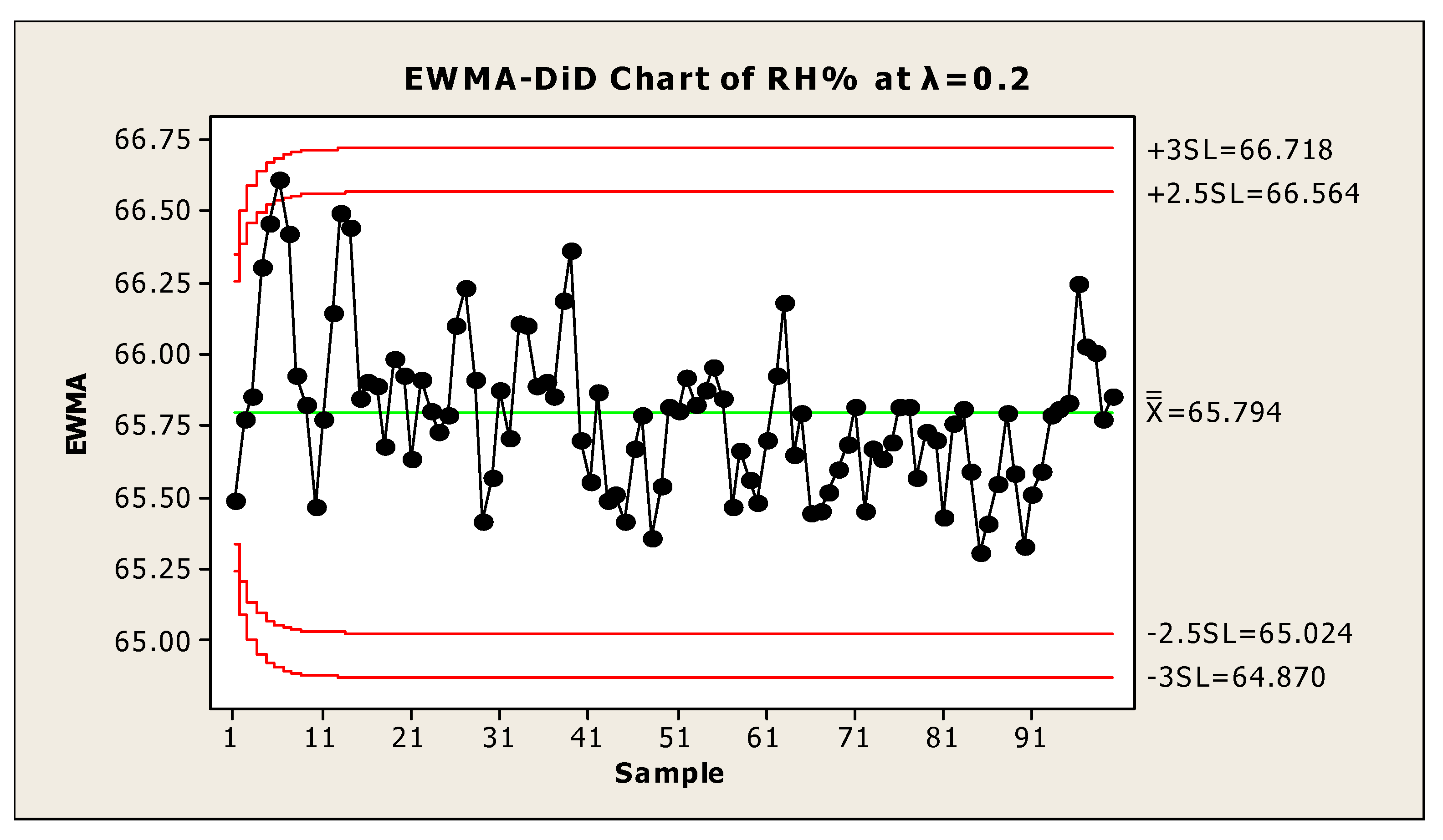
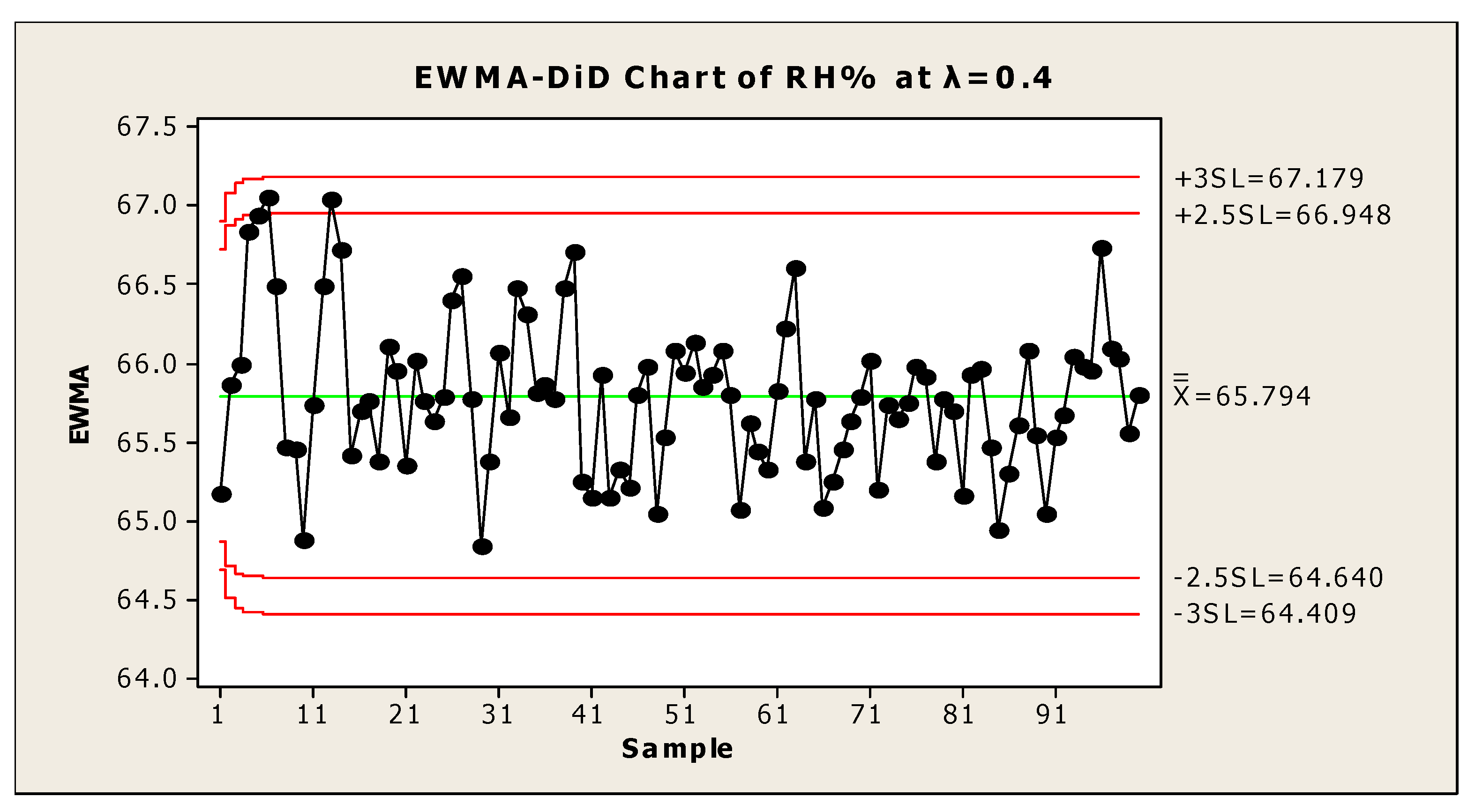
5. Application of Proposed Chart on Real Data Obtained from Industry
6. Conclusions
Author Contributions
Funding
Acknowledgments
Conflicts of Interest
References
- Roberts, S.W. Control Chart Tests Based on Geometric Moving Averages. Technometrics 1959, 1, 239–250. [Google Scholar] [CrossRef]
- Shabbir, J.; Awan, W.H. An efficient Shewhart-Type control chart to monitor moderate size shifts in the process mean in phase-ii. Qual. Reliab. Eng. Int. 2015, 32, 1597–1619. [Google Scholar] [CrossRef]
- Abbas, N.; Riaz, M.; Does, R.J.M.M. Mixed exponentially weighted moving average-cumulative sum charts for process monitoring. Qual. Reliab. Int. 2013, 29, 345–356. [Google Scholar] [CrossRef]
- Haq, A. A new hybrid exponentially weighted moving average control chart for monitoring process mean. Qual. Reliab. Eng. Int. 2013, 29, 1015–1025. [Google Scholar] [CrossRef]
- Lucas, J.M.; Saccucci, M.S. Exponentially Weighted Moving Average Control Schemes: Properties and Enhancements. Technometrics 1990, 32, 1–12. [Google Scholar] [CrossRef]
- Capizzi, G.; Masarotto, G. An adaptive exponentially weighted moving average control chart. Technometrics 2003, 45, 199–207. [Google Scholar] [CrossRef]
- Jiang, W.; Shu, L.; Aplet, D.W. Adaptive CUSUM procedures with EWMA-based shift estimators. IIE Trans. 2008, 40, 992–1003. [Google Scholar]
- Abbasi, S.A.; Miller, A. On Proper Choice of Variability Control Chart for Normal and Non-Normal Processes; John Wiley & Sons, Ltd.: Hoboken, NJ, USA, 2011. [Google Scholar]
- Aslam, M.; Azam, M.; Khan, N.; Jun, C.-H. A mixed control chart to monitor the process. Int. J. Prod. Res. 2015, 53, 4684–4693. [Google Scholar] [CrossRef]
- Azam, M.; Aslam, M.; Jun, C.-H. Designing of a hybrid exponentially weighted moving average control chart using repetitive sampling. Int. J. Adv. Manuf. Technol. 2014, 77, 1927–1933. [Google Scholar]
- Haq, A.; Brown, J.; Moltchanova, E. A new maximum exponentially weighted moving average control chart for monitoring process mean and dispersion. Qual. Reliab. Eng. Int. 2014. [Google Scholar] [CrossRef]
- Haq, A.; Brown, J.; Moltchanova, E.; Al-Omari, A.I. Effect of measurement error on exponentially weighted moving average control charts under ranked set sampling schemes. J. Stat. Comput. Simul. 2014, 85, 1224–1246. [Google Scholar] [CrossRef]
- Aslam, M.; Khan, N.; Aldosari, M.S.; Jun, C.-H. Mixed Control Chart Using EWMA Statistics. IEEE Access 2016, 4, 8286–8293. [Google Scholar] [CrossRef]
- Ali, R.; Haq, A. A mixed GWMA–CUSUM control chart for monitoring the process mean. Commun. Stat. Theory Methods 2018, 47, 3779–3801. [Google Scholar] [CrossRef]
- Sheu, S.H.; Lin, T.C. The generally weighted moving average control chart for detecting small shifts in the process mean. Qual. Eng. 2003, 16, 209–231. [Google Scholar] [CrossRef]
- Ajadi, J.O.; Riaz, M. Mixed multivariate EWMACUSUM control charts for an improved process monitoring. Commun. Stat. Theory Methods 2017, 46, 6980–6993. [Google Scholar] [CrossRef]
- Riaz, M.; Khaliq, Q.-U.-A.; Gul, S. Mixed Tukey EWMA-CUSUM control chart and its applications. Qual. Technol. Quant. Manag. 2017, 14, 378–411. [Google Scholar] [CrossRef]
- Hanif, M.; Hamad, N.; Shahbaz, Q. A modified regression type estimator in survey sampling. World Appl. Sci. J. 2009, 7, 1559–1561. [Google Scholar]
- Hamad, N.; Hanif, M.; Haider, N. A regression type estimator with auxiliary variables for two-phase sampling. Open J. Stat. 2013, 3, 74–78. [Google Scholar] [CrossRef]
- Awan, W.H.; Shabbir, J. On optimum regression estimator for population mean using two auxiliary variables in simple random sampling. Commun. Stat. Simul. Comput. 2014, 43, 1508–1522. [Google Scholar]
- Abbassi, S.A.; Riaz, M. On enhanced control charting for process monitoring. Int. J. Phys. Sci. 2013, 8, 759–775. [Google Scholar]
- Zhang, G.X. Cause-selecting control charts—A new type of control charts. QR J. 1985, 12, 221–225. [Google Scholar]
- Abbas, N.; Riaz, M.; Does, J.M.M.R. An EWMA-Type control chart for monitoring the process mean using auxiliary information. Commun. Stat. Theory Methods 2014, 43, 3485–3498. [Google Scholar] [CrossRef]


| Simple Mean | Ratio Estimator | Classical Regression Estimator | Regression Estimator with Two Auxiliary Variables | Estimator Used in Proposed Chart |
|---|---|---|---|---|
| 100 | 603.37 | 635.08 | 233.37 | 11,620.59 |
| Shift(f) | λ = 0.05 | λ = 0.10 | λ = 0.20 | λ = 0.25 | λ = 1.00 | λ = 0.05 | λ = 0.10 | λ = 0.20 | λ = 0.25 | λ = 1.00 | ||
|---|---|---|---|---|---|---|---|---|---|---|---|---|
| (1) 0.95, 0.95, 0.85 | 0.00 | 375.5 | 374.1 | 368.1 | 349.5 | 355.1 | (7) 0.90, 0.10, 0.52 | 364.1 | 375.0 | 365.3 | 374.7 | 366.8 |
| 0.05 | 18.3 | 20.9 | 27.7 | 32.5 | 130.6 | 4.4 | 5.0 | 5.2 | 5.7 | 21.7 | ||
| 0.10 | 5.6 | 6.4 | 7.3 | 7.6 | 34.6 | 1.6 | 1.7 | 1.8 | 1.9 | 2.8 | ||
| 0.15 | 3.0 | 3.3 | 3.7 | 3.7 | 11.2 | 1.1 | 1.1 | 1.1 | 1.2 | 1.2 | ||
| 0.20 | 2.0 | 2.2 | 2.3 | 2.3 | 4.5 | 1.0 | 1.0 | 1.0 | 1.0 | 1.0 | ||
| 0.35 | 1.1 | 1.1 | 1.2 | 1.2 | 1.2 | 1.0 | 1.0 | 1.0 | 1.0 | 1.0 | ||
| 0.50 | 1.0 | 1.0 | 1.0 | 1.0 | 1.0 | 1.0 | 1.0 | 1.0 | 1.0 | 1.0 | ||
| 0.75 | 1.0 | 1.0 | 1.0 | 1.0 | 1.0 | 1.0 | 1.0 | 1.0 | 1.0 | 1.0 | ||
| 1.00 | 1.0 | 1.0 | 1.0 | 1.0 | 1.0 | 1.0 | 1.0 | 1.0 | 1.0 | 1.0 | ||
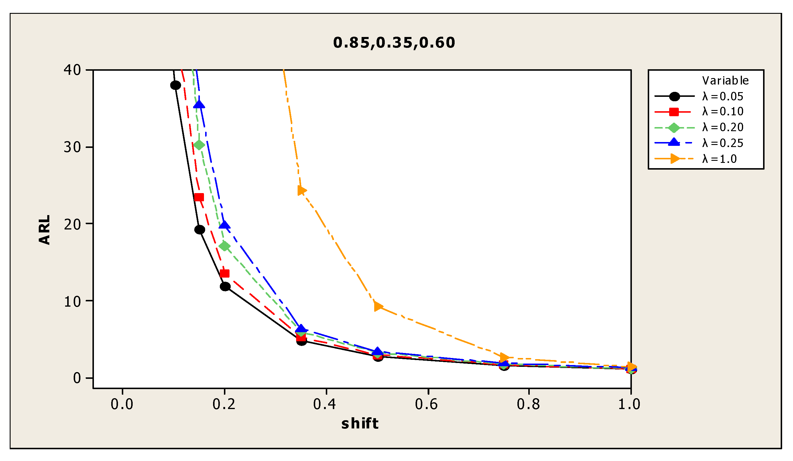
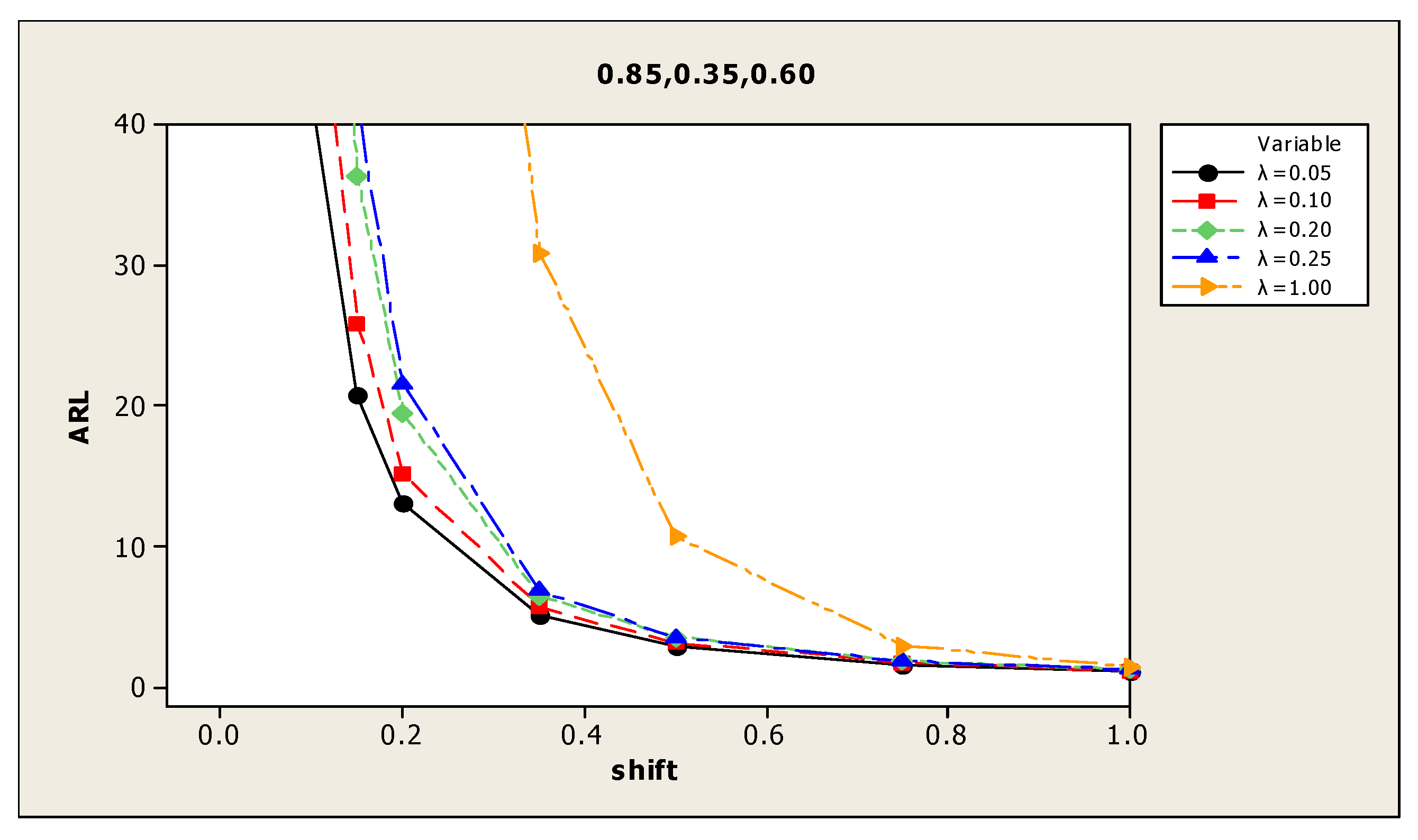
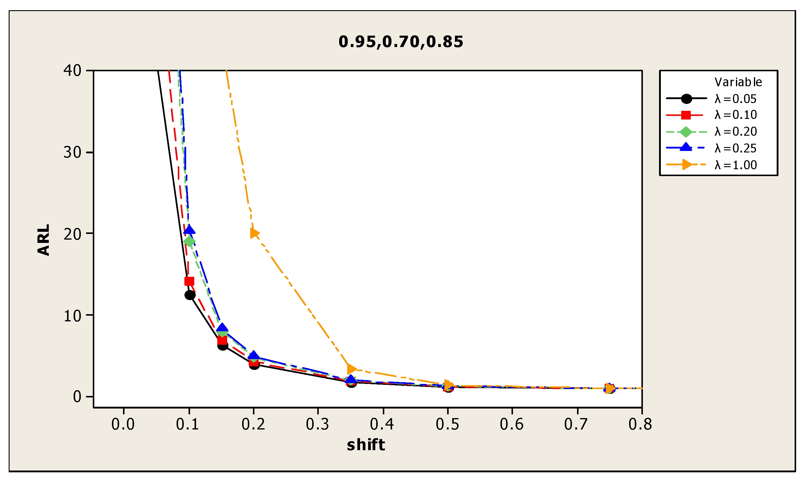
| (2) 0.95, 0.70, 0.85 | 0.00 | 370.7 | 366.1 | 347.9 | 374.9 | 369.2 | (8) 0.85, 0.35, 0.60 | 375.4 | 370.8 | 355.2 | 367.3 | 358.1 |
| 0.05 | 36.1 | 45.1 | 61.2 | 72.6 | 215.0 | 109.6 | 146.6 | 179.3 | 186.6 | 316.3 | ||
| 0.10 | 11.1 | 13.3 | 15.6 | 18.4 | 85.6 | 38.1 | 47.4 | 65.6 | 78.0 | 216.4 | ||
| 0.15 | 6.1 | 6.6 | 7.4 | 7.7 | 34.1 | 19.3 | 23.4 | 30.3 | 35.4 | 139.0 | ||
| 0.20 | 3.6 | 4.1 | 4.5 | 4.7 | 16.2 | 12.0 | 13.6 | 17.1 | 19.8 | 90.1 | ||
| 0.35 | 1.7 | 1.8 | 1.9 | 1.9 | 3.0 | 4.8 | 5.3 | 6.0 | 6.4 | 24.4 | ||
| 0.50 | 1.1 | 1.2 | 1.2 | 1.2 | 1.3 | 2.8 | 3.0 | 3.3 | 3.4 | 9.3 | ||
| 0.75 | 1.0 | 1.0 | 1.0 | 1.0 | 1.0 | 1.6 | 1.7 | 1.8 | 1.9 | 2.7 | ||
| 1.00 | 1.0 | 1.0 | 1.0 | 1.0 | 1.0 | 1.2 | 1.2 | 1.2 | 1.3 | 1.4 | ||
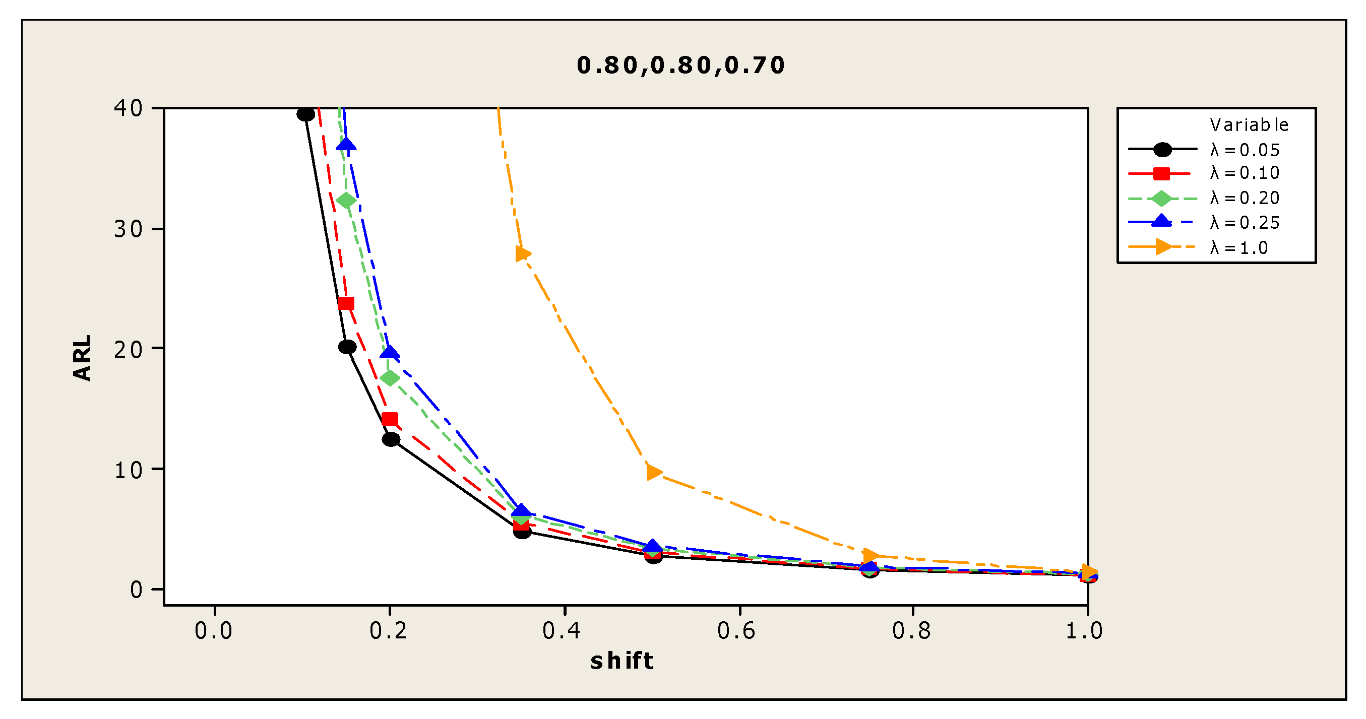
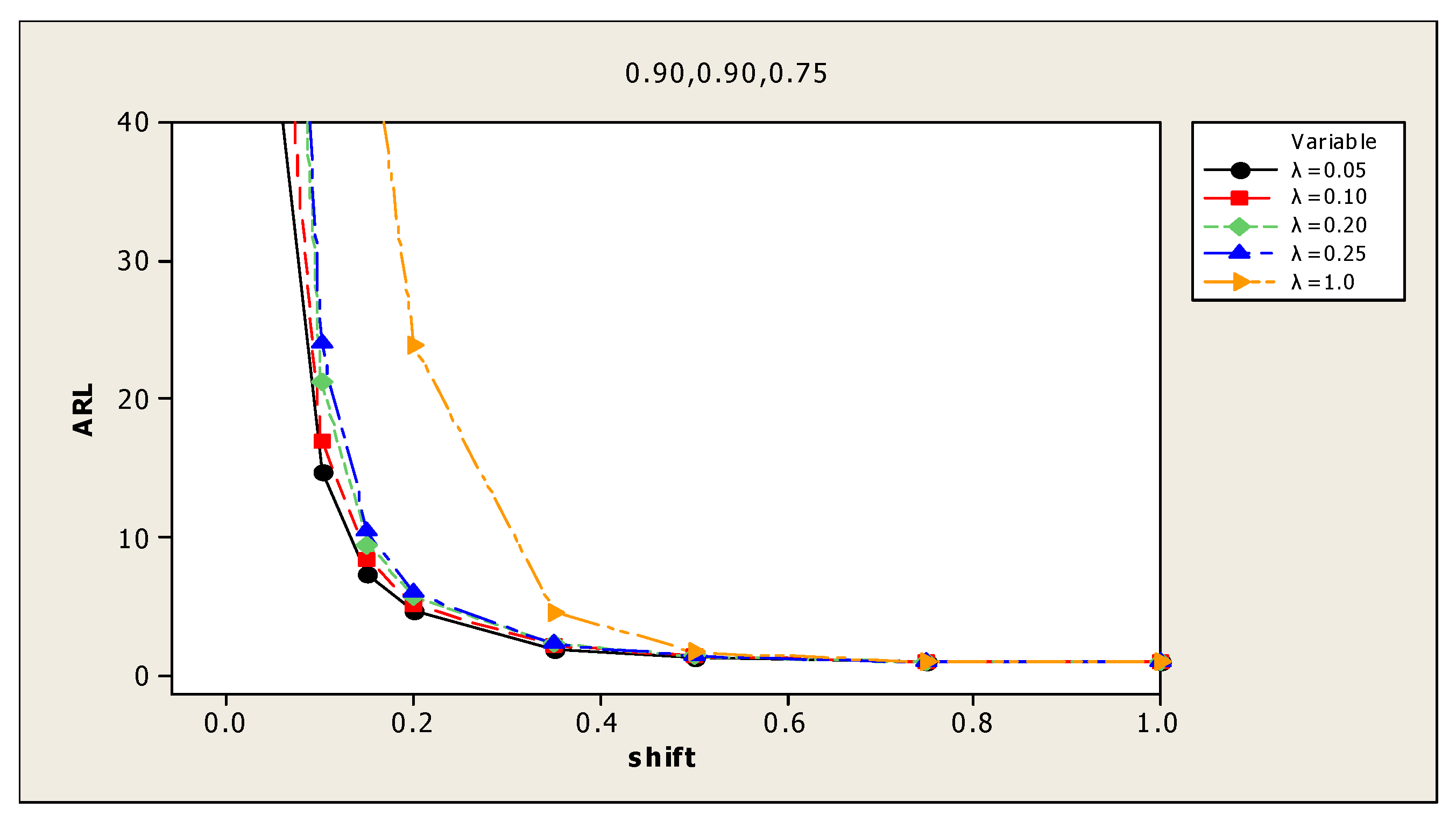
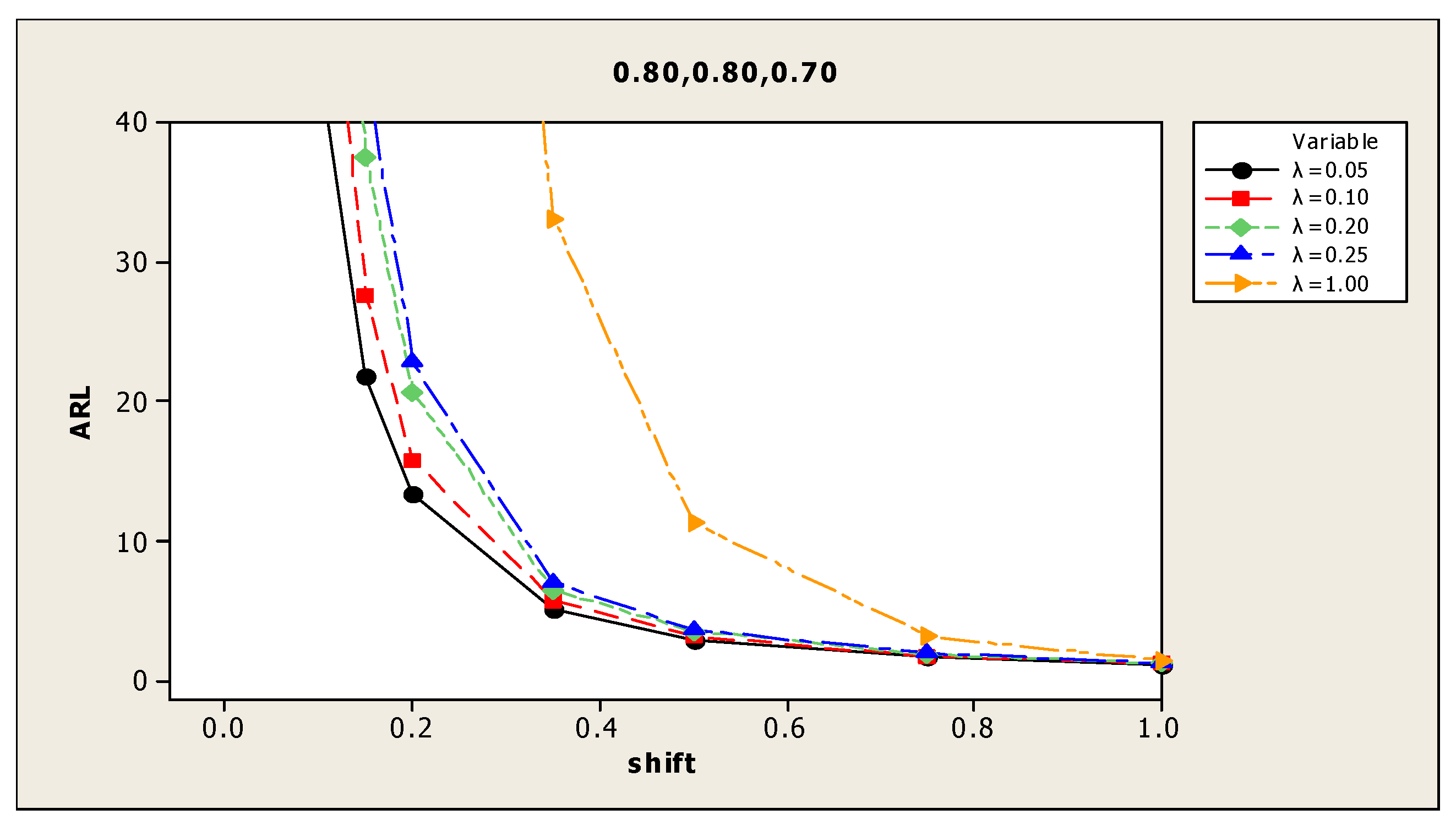
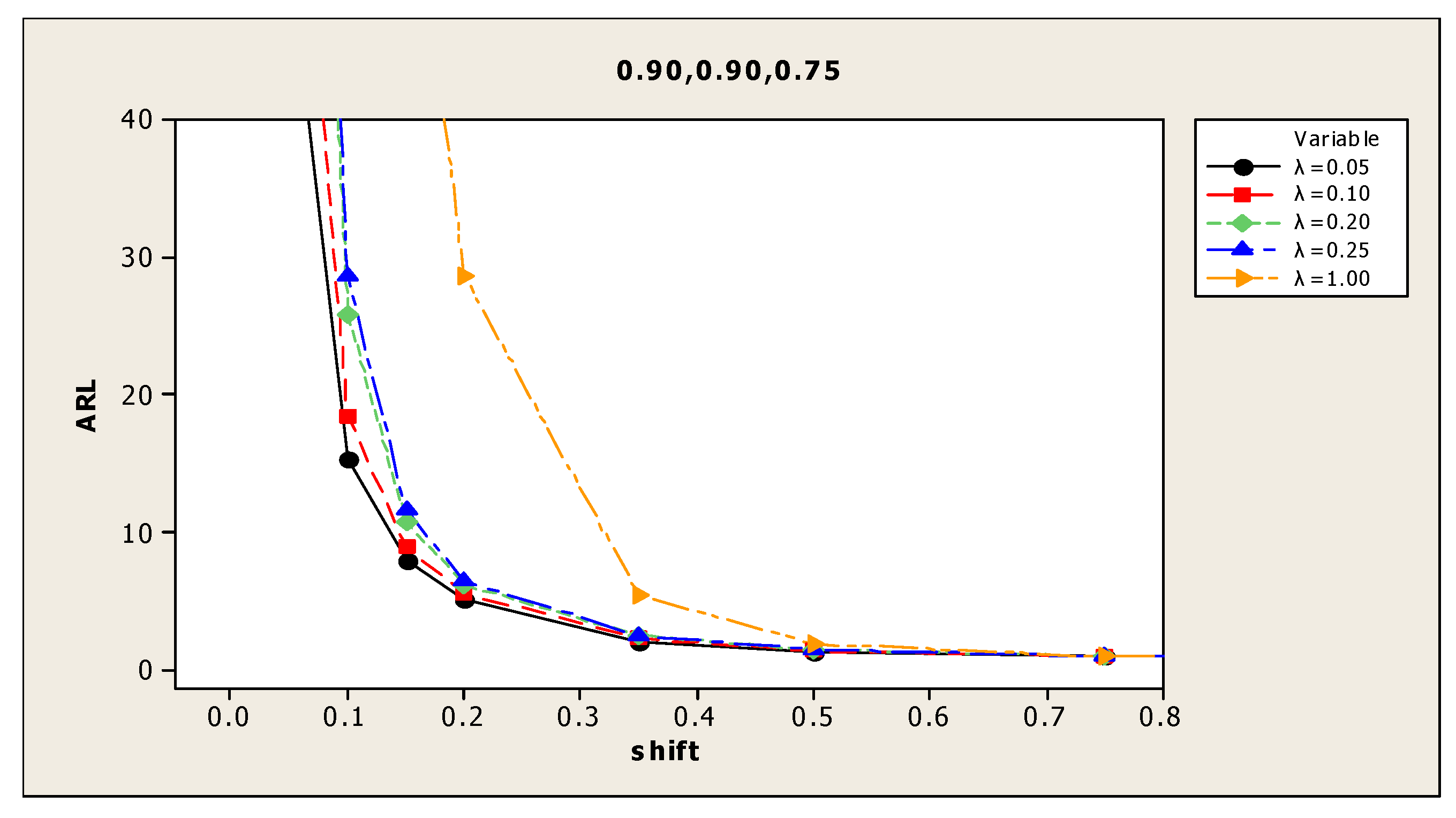
| (3) 0.90, 0.90, 0.75 | 0.00 | 376.0 | 368.0 | 371.6 | 365.6 | 365.5 | (9) 0.80, 0.80, 0.70 | 388.4 | 360.1 | 364.0 | 375.0 | 358.9 |
| 0.05 | 45.5 | 56.6 | 82.0 | 94.0 | 250.3 | 115.9 | 140.8 | 185.7 | 204.4 | 331.1 | ||
| 0.10 | 14.7 | 17.0 | 21.3 | 24.0 | 111.1 | 39.5 | 48.7 | 69.7 | 79.1 | 225.5 | ||
| 0.15 | 7.3 | 8.4 | 9.5 | 10.4 | 48.5 | 20.2 | 23.8 | 32.3 | 36.9 | 148.6 | ||
| 0.20 | 4.7 | 5.1 | 5.7 | 6.0 | 23.9 | 12.5 | 14.1 | 17.6 | 19.6 | 93.0 | ||
| 0.35 | 1.9 | 2.2 | 2.3 | 2.3 | 4.6 | 4.9 | 5.5 | 6.1 | 6.5 | 27.9 | ||
| 0.50 | 1.3 | 1.4 | 1.4 | 1.4 | 1.7 | 2.8 | 3.1 | 3.4 | 3.6 | 9.7 | ||
| 0.75 | 1.0 | 1.0 | 1.0 | 1.0 | 1.0 | 1.6 | 1.7 | 1.8 | 1.9 | 2.8 | ||
| 1.00 | 1.0 | 1.0 | 1.0 | 1.0 | 1.0 | 1.2 | 1.2 | 1.3 | 1.3 | 1.4 | ||
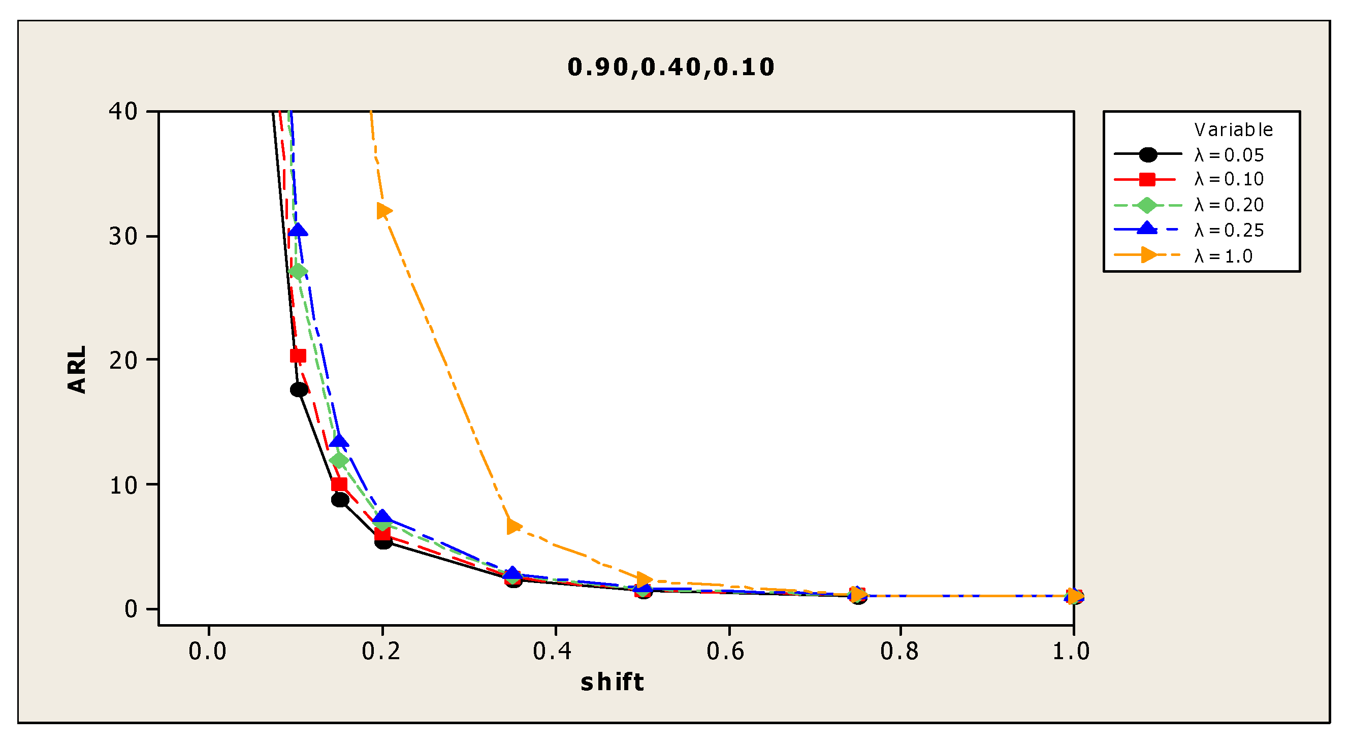
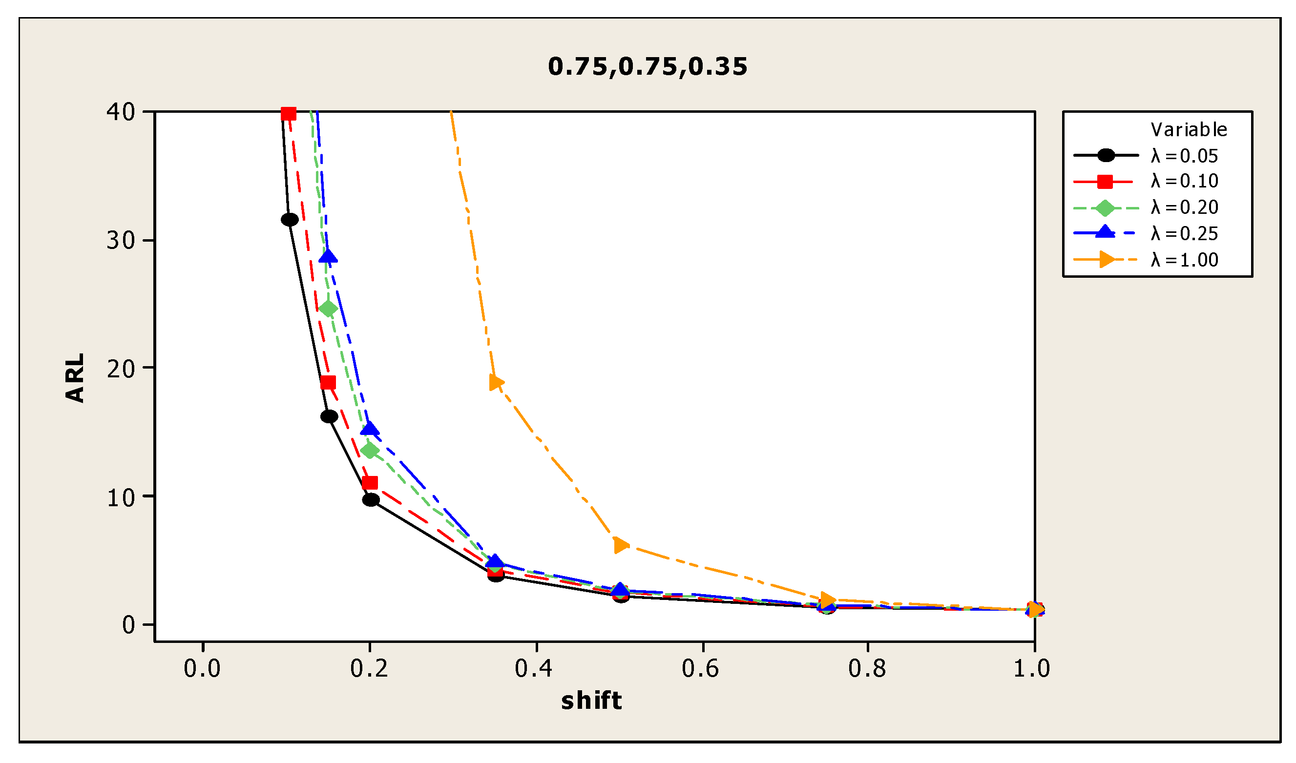
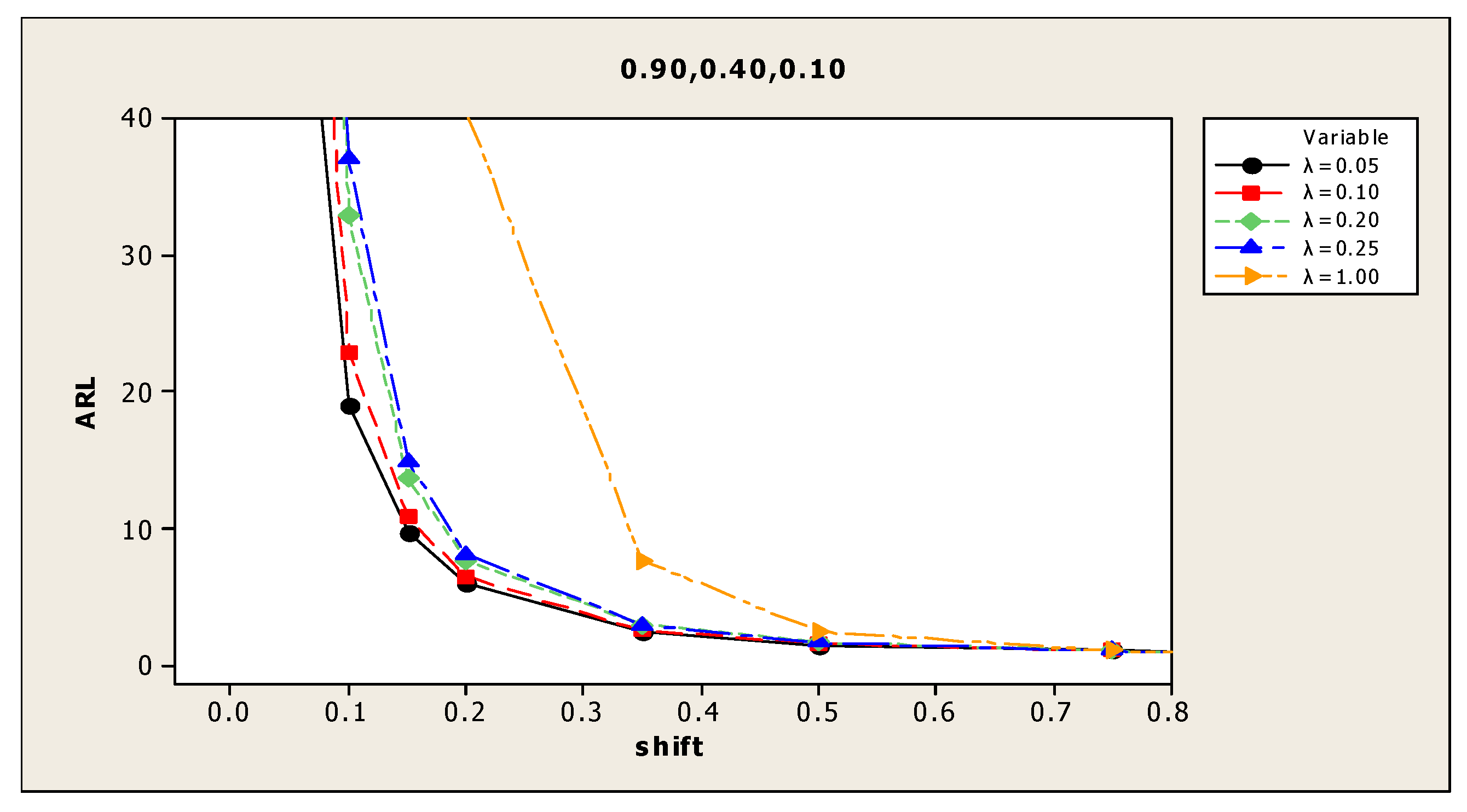
| (4) 0.90, 0.40, 0.10 | 0.00 | 359.7 | 374.7 | 359.2 | 363.6 | 372.3 | (10) 0.75, 0.75, 0.35 | 381.2 | 367.8 | 361.0 | 365.1 | 362.7 |
| 0.05 | 56.3 | 70.4 | 97.6 | 113.6 | 265.1 | 90.0 | 108.2 | 150.8 | 165.7 | 301.5 | ||
| 0.10 | 17.7 | 20.4 | 27.2 | 30.4 | 124.4 | 28.3 | 35.3 | 49.4 | 54.8 | 195.9 | ||
| 0.15 | 8.9 | 10.1 | 11.9 | 13.4 | 60.4 | 14.2 | 16.6 | 22.2 | 25.1 | 106.0 | ||
| 0.20 | 5.5 | 6.0 | 6.9 | 7.4 | 32.0 | 8.9 | 10.1 | 11.7 | 13.5 | 66.8 | ||
| 0.35 | 2.3 | 2.5 | 2.7 | 2.8 | 6.6 | 3.5 | 4.0 | 4.4 | 4.5 | 15.3 | ||
| 0.50 | 1.4 | 1.5 | 1.6 | 1.7 | 2.3 | 2.1 | 2.3 | 2.5 | 2.6 | 5.3 | ||
| 0.75 | 1.0 | 1.1 | 1.1 | 1.1 | 1.1 | 1.3 | 1.4 | 1.4 | 1.4 | 1.7 | ||
| 1.00 | 1.0 | 1.0 | 1.0 | 1.0 | 1.0 | 1.0 | 1.1 | 1.1 | 1.1 | 1.1 | ||
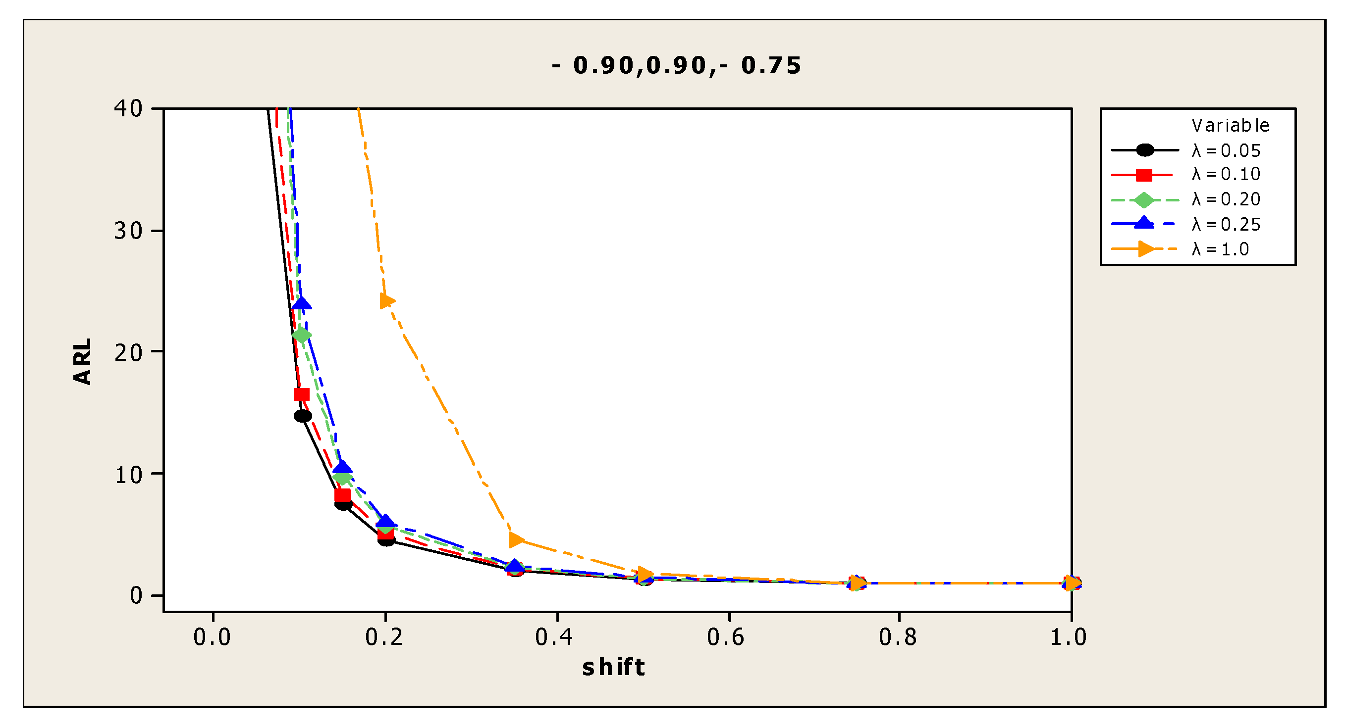
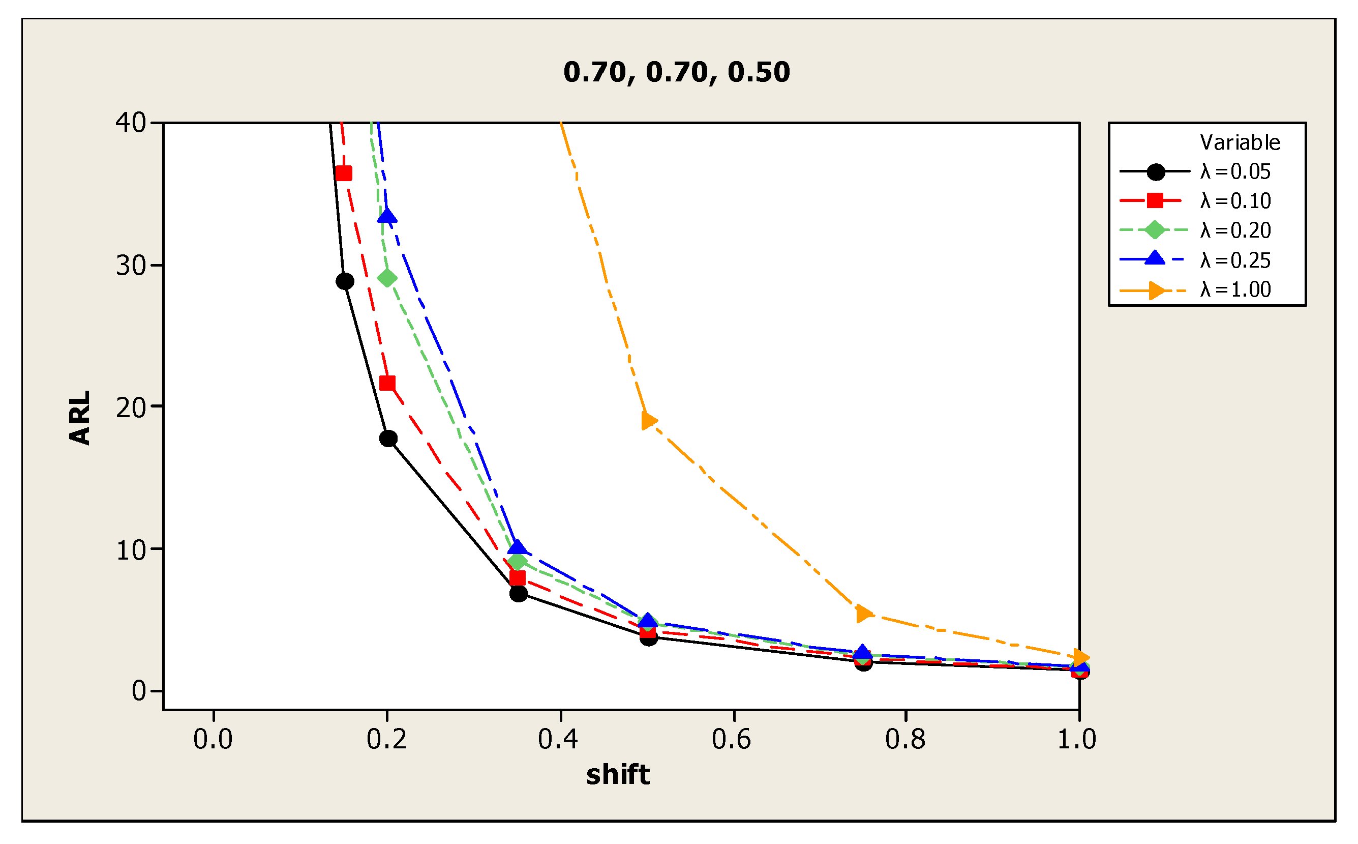
| (5) 0.70, 0.70, 0.50 | 0.00 | 373.0 | 359.8 | 359.0 | 371.0 | 378.5 | (11) −0.90, 0.90, −0.75 | 370.8 | 373.7 | 373.0 | 357.3 | 357.4 |
| 0.05 | 145.3 | 173.3 | 208.6 | 227.1 | 326.7 | 46.6 | 57.9 | 80.7 | 94.6 | 239.5 | ||
| 0.10 | 53.6 | 68.0 | 90.5 | 109.6 | 248.6 | 14.8 | 16.5 | 21.4 | 23.9 | 107.0 | ||
| 0.15 | 27.3 | 32.5 | 44.3 | 49.6 | 185.5 | 7.5 | 8.3 | 9.8 | 10.5 | 49.2 | ||
| 0.20 | 16.5 | 19.2 | 25.0 | 27.4 | 126.3 | 4.6 | 5.1 | 5.7 | 6.1 | 24.2 | ||
| 0.35 | 6.3 | 7.1 | 8.4 | 8.8 | 41.4 | 2.0 | 2.2 | 2.3 | 2.4 | 4.6 | ||
| 0.50 | 3.6 | 4.0 | 4.5 | 4.7 | 15.5 | 1.3 | 1.4 | 1.4 | 1.5 | 1.8 | ||
| 0.75 | 2.0 | 2.2 | 2.3 | 2.4 | 4.6 | 1.0 | 1.0 | 1.0 | 1.0 | 1.0 | ||
| 1.00 | 1.4 | 1.5 | 1.6 | 1.6 | 2.1 | 1.0 | 1.0 | 1.0 | 1.0 | 1.0 | ||
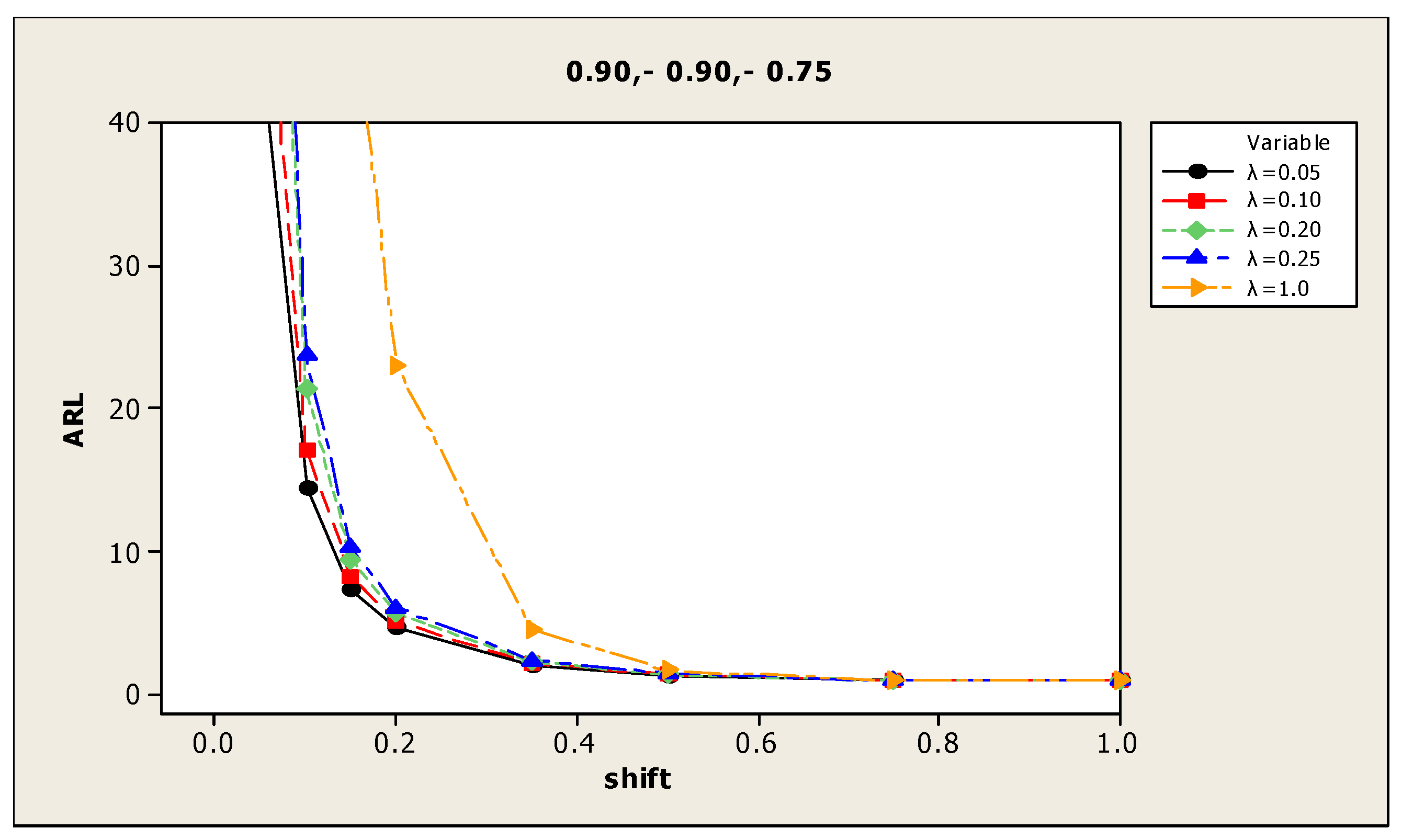
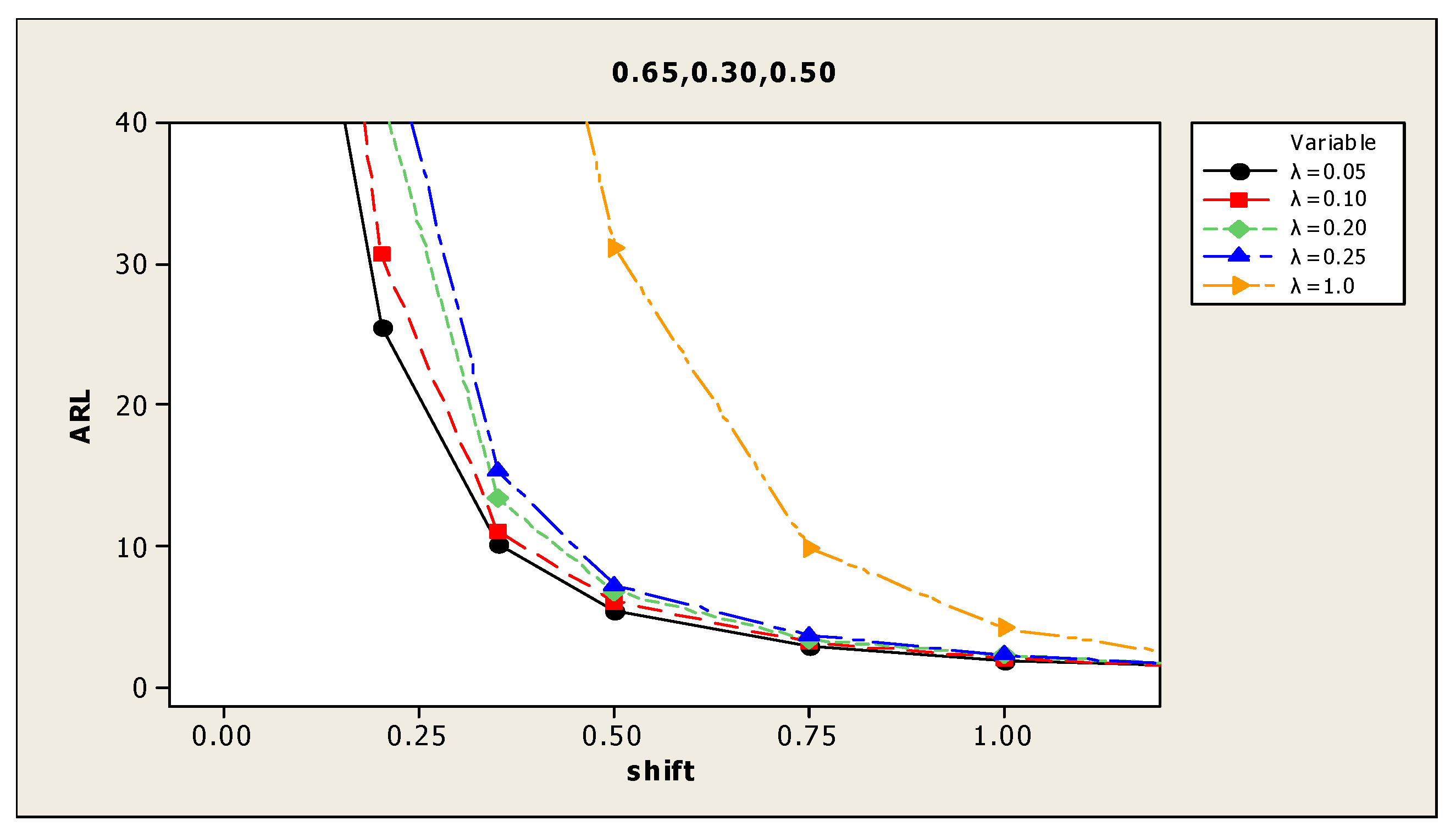
| (6) 0.65, 0.30, 0.50 | 0.00 | 369.2 | 382.1 | 359.9 | 359.6 | 367.4 | (12) 0.90, −0.90, −0.75 | 387.2 | 380.6 | 350.2 | 367.5 | 364.0 |
| 0.05 | 188.7 | 225.1 | 257.2 | 274.9 | 350.1 | 45.9 | 57.2 | 83.9 | 93.5 | 242.0 | ||
| 0.10 | 77.6 | 100.7 | 130.1 | 146.9 | 297.1 | 14.4 | 17.1 | 21.4 | 23.8 | 107.4 | ||
| 0.15 | 40.7 | 51.3 | 70.6 | 80.0 | 237.4 | 7.3 | 8.3 | 9.4 | 10.3 | 49.4 | ||
| 0.20 | 25.6 | 30.7 | 42.0 | 48.8 | 165.9 | 4.7 | 5.1 | 5.7 | 6.1 | 23.0 | ||
| 0.35 | 10.2 | 11.1 | 13.4 | 15.4 | 68.9 | 2.0 | 2.2 | 2.3 | 2.4 | 4.6 | ||
| 0.50 | 5.5 | 6.1 | 6.8 | 7.2 | 31.1 | 1.3 | 1.4 | 1.4 | 1.5 | 1.7 | ||
| 0.75 | 2.9 | 3.2 | 3.4 | 3.7 | 9.9 | 1.0 | 1.0 | 1.0 | 1.0 | 1.0 | ||
| 1.00 | 1.9 | 2.1 | 2.3 | 2.3 | 4.2 | 1.0 | 1.0 | 1.0 | 1.0 | 1.0 |
| Shift(f) | λ = 0.05 | λ = 0.10 | λ = 0.20 | λ = 0.25 | λ = 1.00 | λ = 0.05 | λ = 0.10 | λ = 0.20 | λ = 0.25 | λ = 1.00 | ||
|---|---|---|---|---|---|---|---|---|---|---|---|---|
| (1) 0.95, 0.95, 0.85 | 0.00 | 508.7 | 490.9 | 521.9 | 478.7 | 489.6 | (7) 0.90, 0.10, 0.52 | 499.8 | 478.4 | 508.7 | 491.7 | 490.1 |
| 0.05 | 20.0 | 23.7 | 33.8 | 37.8 | 173.9 | 4.8 | 5.2 | 5.8 | 6.1 | 26.8 | ||
| 0.10 | 6.3 | 6.8 | 7.9 | 8.4 | 41.3 | 1.7 | 1.8 | 1.9 | 2.0 | 3.2 | ||
| 0.15 | 3.2 | 3.6 | 3.8 | 4.0 | 13.1 | 1.1 | 1.1 | 1.2 | 1.2 | 1.3 | ||
| 0.20 | 2.1 | 2.3 | 2.5 | 2.5 | 5.0 | 1.0 | 1.0 | 1.0 | 1.0 | 1.0 | ||
| 0.35 | 1.1 | 1.1 | 1.2 | 1.2 | 1.3 | 1.0 | 1.0 | 1.0 | 1.0 | 1.0 | ||
| 0.50 | 1.0 | 1.0 | 1.0 | 1.0 | 1.0 | 1.0 | 1.0 | 1.0 | 1.0 | 1.0 | ||
| 0.75 | 1.0 | 1.0 | 1.0 | 1.0 | 1.0 | 1.0 | 1.0 | 1.0 | 1.0 | 1.0 | ||
| 1.00 | 1.0 | 1.0 | 1.0 | 1.0 | 1.0 | 1.0 | 1.0 | 1.0 | 1.0 | 1.0 | ||
| (2) 0.95, 0.70, 0.85 | 0.00 | 506.0 | 478.7 | 508.1 | 485.5 | 484.0 | (8) 0.85, 0.35, 0.60 | 487.9 | 479.4 | 515.5 | 502.1 | 485.7 |
| 0.05 | 41.0 | 54.0 | 78.9 | 90.5 | 292.9 | 138.9 | 173.8 | 255.2 | 270.1 | 426.6 | ||
| 0.10 | 12.5 | 14.1 | 19.1 | 20.4 | 109.9 | 41.3 | 55.6 | 86.3 | 94.9 | 286.3 | ||
| 0.15 | 6.4 | 7.0 | 8.0 | 8.4 | 43.2 | 20.8 | 25.9 | 36.3 | 41.3 | 187.7 | ||
| 0.20 | 4.0 | 4.3 | 4.8 | 5.0 | 20.1 | 13.2 | 15.2 | 19.5 | 21.6 | 119.0 | ||
| 0.35 | 1.7 | 1.9 | 2.0 | 2.0 | 3.4 | 5.1 | 5.7 | 6.5 | 6.9 | 30.9 | ||
| 0.50 | 1.2 | 1.2 | 1.3 | 1.3 | 1.4 | 2.9 | 3.2 | 3.6 | 3.6 | 10.7 | ||
| 0.75 | 1.0 | 1.0 | 1.0 | 1.0 | 1.0 | 1.6 | 1.8 | 1.9 | 1.9 | 3.0 | ||
| 1.00 | 1.0 | 1.0 | 1.0 | 1.0 | 1.0 | 1.2 | 1.2 | 1.3 | 1.3 | 1.5 | ||
| (3) 0.90, 0.90, 0.75 | 0.00 | 493.9 | 490.7 | 533.6 | 494.9 | 498.0 | (9) 0.80, 0.80, 0.70 | 485.0 | 475.5 | 495.2 | 495.2 | 482.5 |
| 0.05 | 51.7 | 68.8 | 109.3 | 117.9 | 329.9 | 138.6 | 181.2 | 256.7 | 278.6 | 429.6 | ||
| 0.10 | 15.3 | 18.5 | 25.9 | 28.7 | 146.1 | 44.0 | 60.2 | 86.3 | 98.2 | 305.5 | ||
| 0.15 | 8.0 | 9.0 | 10.7 | 11.6 | 61.8 | 21.9 | 27.6 | 37.5 | 43.9 | 188.4 | ||
| 0.20 | 5.1 | 5.6 | 6.2 | 6.5 | 28.7 | 13.4 | 15.8 | 20.7 | 22.8 | 118.9 | ||
| 0.35 | 2.1 | 2.3 | 2.5 | 2.5 | 5.4 | 5.2 | 5.8 | 6.5 | 7.1 | 33.1 | ||
| 0.50 | 1.3 | 1.4 | 1.5 | 1.5 | 1.9 | 3.0 | 3.2 | 3.6 | 3.7 | 11.3 | ||
| 0.75 | 1.0 | 1.0 | 1.0 | 1.0 | 1.0 | 1.7 | 1.8 | 1.9 | 2.0 | 3.2 | ||
| 1.00 | 1.0 | 1.0 | 1.0 | 1.0 | 1.0 | 1.2 | 1.3 | 1.3 | 1.3 | 1.5 | ||
| (4) 0.90, 0.40, 0.10 | 0.00 | 461.8 | 480.6 | 499.1 | 489.2 | 481.8 | (10) 0.75, 0.75, 0.35 | 487.0 | 486.5 | 501.6 | 487.5 | 488.0 |
| 0.05 | 65.0 | 86.5 | 127.9 | 137.1 | 348.7 | 100.8 | 135.3 | 193.9 | 222.5 | 424.0 | ||
| 0.10 | 19.1 | 22.9 | 32.9 | 37.0 | 173.4 | 31.6 | 39.9 | 60.2 | 67.7 | 246.1 | ||
| 0.15 | 9.7 | 10.9 | 13.7 | 14.9 | 80.6 | 16.2 | 18.9 | 24.6 | 28.6 | 140.5 | ||
| 0.20 | 6.1 | 6.5 | 7.7 | 8.1 | 40.4 | 9.7 | 11.0 | 13.6 | 15.2 | 78.6 | ||
| 0.35 | 2.5 | 2.6 | 3.0 | 3.0 | 7.7 | 3.9 | 4.2 | 4.7 | 4.8 | 18.9 | ||
| 0.50 | 1.5 | 1.6 | 1.7 | 1.7 | 2.5 | 2.2 | 2.5 | 2.6 | 2.7 | 6.2 | ||
| 0.75 | 1.1 | 1.1 | 1.1 | 1.1 | 1.1 | 1.3 | 1.4 | 1.5 | 1.5 | 1.9 | ||
| 1.00 | 1.0 | 1.0 | 1.0 | 1.0 | 1.0 | 1.1 | 1.1 | 1.1 | 1.1 | 1.1 | ||
| (5) 0.70, 0.70, 0.50 | 0.00 | 488.9 | 498.3 | 520.7 | 495.9 | 507.6 | (11) −0.90, 0.90, −0.75 | 484.4 | 476.7 | 505.3 | 508.4 | 490.3 |
| 0.05 | 174.5 | 222.7 | 311.6 | 323.5 | 417.8 | 51.3 | 67.9 | 102.5 | 116.4 | 330.6 | ||
| 0.10 | 59.3 | 80.2 | 119.4 | 138.2 | 346.8 | 15.8 | 18.6 | 24.4 | 28.3 | 137.9 | ||
| 0.15 | 29.0 | 36.4 | 55.7 | 63.2 | 237.6 | 8.0 | 9.0 | 10.7 | 11.6 | 60.6 | ||
| 0.20 | 17.8 | 21.7 | 29.1 | 33.3 | 155.2 | 4.9 | 5.4 | 6.3 | 6.4 | 29.1 | ||
| 0.35 | 7.0 | 7.9 | 9.2 | 10.1 | 50.7 | 2.1 | 2.3 | 2.5 | 2.5 | 5.2 | ||
| 0.50 | 3.9 | 4.3 | 4.8 | 4.9 | 19.0 | 1.3 | 1.4 | 1.5 | 1.5 | 1.9 | ||
| 0.75 | 2.1 | 2.3 | 2.5 | 2.6 | 5.4 | 1.0 | 1.0 | 1.0 | 1.0 | 1.1 | ||
| 1.00 | 1.5 | 1.5 | 1.7 | 1.7 | 2.3 | 1.0 | 1.0 | 1.0 | 1.0 | 1.0 | ||
| (6) 0.65, 0.30, 0.50 | 0.00 | 489.9 | 507.5 | 506.1 | 486.0 | 493.2 | (12) 0.90, −0.90, −0.75 | 488.0 | 478.9 | 516.1 | 477.2 | 492.1 |
| 0.05 | 236.4 | 290.7 | 358.0 | 393.0 | 471.0 | 53.2 | 68.6 | 105.7 | 117.2 | 337.2 | ||
| 0.10 | 92.0 | 120.9 | 176.3 | 197.8 | 386.3 | 16.1 | 17.8 | 25.3 | 27.8 | 136.4 | ||
| 0.15 | 46.2 | 61.9 | 89.3 | 104.0 | 311.4 | 7.9 | 8.9 | 10.8 | 11.6 | 59.1 | ||
| 0.20 | 28.6 | 33.8 | 53.5 | 57.9 | 228.4 | 4.9 | 5.5 | 6.3 | 6.5 | 28.8 | ||
| 0.35 | 10.9 | 12.0 | 15.4 | 16.6 | 92.5 | 2.1 | 2.3 | 2.5 | 2.5 | 5.1 | ||
| 0.50 | 5.9 | 6.7 | 7.9 | 7.9 | 39.7 | 1.3 | 1.4 | 1.5 | 1.5 | 1.9 | ||
| 0.75 | 3.0 | 3.4 | 3.7 | 3.8 | 11.6 | 1.0 | 1.0 | 1.0 | 1.0 | 1.1 | ||
| 1.00 | 2.0 | 2.2 | 2.4 | 2.4 | 4.8 | 1.0 | 1.0 | 1.0 | 1.0 | 1.0 |
| Shift | CUSUM k = 0.5 | EWMA Chart | EWMA-DiD | ||||||
|---|---|---|---|---|---|---|---|---|---|
| λ = 0.05 | λ = 0.1 | λ = 0.2 | λ = 0.25 | λ = 0.5 | |||||
| 0.00 | 500.5 | 502.8 | 499.9 | 499.8 | 499.6 | 500.0 | 500.5 | 495.8 | 490.1 |
| 0.25 | 241.2 | 52.4 | 35.5 | 40.5 | 55.8 | 64.8 | 116.9 | <13.0 | 78.1 |
| 0.50 | 76.2 | 13.4 | 13.6 | 12.7 | 13.7 | 14.9 | 25.1 | <3.7 | 11.3 |
| 0.75 | 27.3 | 7.1 | 8.3 | 7.3 | 6.8 | 6.9 | 9.1 | <2.0 | 3.2 |
| 1.00 | 11.5 | 4.8 | 6.1 | 5.1 | 4.5 | 4.4 | 4.8 | <1.3 | 1.5 |
| 1.50 | 3.2 | 3.0 | 4.0 | 3.3 | 2.8 | 2.6 | 2.4 | 1.0 | 1.0 |
| 2.00 | 1.5 | 2.3 | 3.1 | 2.5 | 2.1 | 2.0 | 1.6 | 1.0 | 1.0 |
| 2.50 | 1.1 | 1.9 | 2.5 | 2.1 | 1.7 | 1.6 | 1.2 | 1.0 | 1.0 |
| 3.00 | 1.0 | 1.6 | 2.1 | 1.9 | 1.4 | 1.3 | 1.0 | 1.0 | 1.0 |
| Variables | Parameters | Variable Type | ||
|---|---|---|---|---|
| RH% | Quality Concern | |||
| Amb TC | Auxiliary Information | |||
| Amb RH | ||||
© 2018 by the authors. Licensee MDPI, Basel, Switzerland. This article is an open access article distributed under the terms and conditions of the Creative Commons Attribution (CC BY) license (http://creativecommons.org/licenses/by/4.0/).
Share and Cite
Mughal, M.A.; Azam, M.; Aslam, M. An EWMA-DiD Control Chart to Capture Small Shifts in the Process Average Using Auxiliary Information. Technologies 2018, 6, 69. https://doi.org/10.3390/technologies6030069
Mughal MA, Azam M, Aslam M. An EWMA-DiD Control Chart to Capture Small Shifts in the Process Average Using Auxiliary Information. Technologies. 2018; 6(3):69. https://doi.org/10.3390/technologies6030069
Chicago/Turabian StyleMughal, Muhammad Anwar, Muhammad Azam, and Muhammad Aslam. 2018. "An EWMA-DiD Control Chart to Capture Small Shifts in the Process Average Using Auxiliary Information" Technologies 6, no. 3: 69. https://doi.org/10.3390/technologies6030069
APA StyleMughal, M. A., Azam, M., & Aslam, M. (2018). An EWMA-DiD Control Chart to Capture Small Shifts in the Process Average Using Auxiliary Information. Technologies, 6(3), 69. https://doi.org/10.3390/technologies6030069