Article

An EWMA-DiD Control Chart to Capture Small Shifts in the Process Average Using Auxiliary Information

by
Muhammad Anwar Mughal
1,
Muhammad Azam
2 and
Muhammad Aslam
3,*
1
Department of Statistics, National College of Business Administration & Economics, Lahore 54660, Pakistan
2
Department of Statistics and Computer Science, University of Veterinary and Animal Sciences, Lahore 54000, Pakistan
3
Department of Statistics, Faculty of Science, King Abdulaziz University, Jeddah 21551, Saudi Arabia
*
Author to whom correspondence should be addressed.
Technologies 2018, 6(3), 69; https://doi.org/10.3390/technologies6030069
Submission received: 29 May 2018 / Revised: 18 July 2018 / Accepted: 23 July 2018 / Published: 30 July 2018

Abstract

:
Among the Statistical Process Control (SPC) techniques, control charts are considered to be high weight-age due to their effectiveness in process variation. As the Shewhart’s charts are not that active in monitoring small and moderate process variations, the statisticians have been making efforts to improve the performance of the control chart by introducing several techniques within the tool. These techniques consist of experimenting with different estimators, different sampling selection techniques, and mixed methodologies. The proposed chart is one of the examples of a mixed chart technique that has shown its efficiency in monitoring small variations better than any of the existing techniques in the specific situation of auxiliary information. To show and compare its performance, average run length (ARL) tables and ARL curves have been presented in the article. An industrial example has also been included to show the practical application of the proposed chart in a real scenario.

1. Introduction

Statistical Process Control (SPC) contains a set of tools that are widely used for improving process performance by reducing the variability in the key process parameters. These tools have been found to be very useful in achieving process stability and improving process capability. It is one of the greatest developments of the twentieth century. Because of sound underlying principles, it can be applied to any process. Among the seven SPC tools, Walter A. Shewhart of the Bell Telephone Company developed Shewhart control charts. These charts are commonly used in Phase-I implementation of SPC to monitor the process when there is large shift in parameters.
A major objective of SPC is to quickly detect the occurrence of an assignable cause or non-random cause of process shifts so that root cause analysis of the process and corrective action may be addressed to avoid nonconforming items in the manufacturing process. These techniques are widely used as online process monitoring techniques. The main purpose of the process control is to reduce the variability if it cannot be completely eliminated. The control charts have been found highly effective to reduce the variability in the process.
One of the disadvantages of the Shewhart control chart is that it utilizes only information contained in the last sample and ignores the information lying in the earlier subgroups. This feature makes these charts less sensitive to small shifts. Accordingly, they are less useful in process control when detection of small shifts is important. Moreover, in the modern competitive era of industry and the precise requirements of the customer, these control charts are not that effective, which is due to their flexibility. These charts may present the process in a well-controlled scenario, whereas actually non-conforming items are also being produced. Today the industry focuses on Lean Processes to decrease waste and increase productivity and profitability.
In this situation, the process demands very sensitive monitoring that is capable of detecting a minor variation in controllable characteristics. This tendency has created new challenges for control chart developers to develop more sensitive monitoring techniques. To capture minor shifts in the processes, the most popular charts found in the literature are CUSUM and exponentially weighted moving average chart (EWMA) control charts.
In the recent literature, the EWMA chart is more popular as a result of its appealing mechanism that enables the user to adjust the weight-age of recent and previous data obtained from the process. Roberts [1] introduced the EWMA statistic to construct a control chart for monitoring small and moderate shifts in the process. It has the quality to embed any estimator to make the chart more useful and sensitive in terms of its performance. In this article, an EWMA-DiD control chart has been proposed to monitor small shifts in process average. This chart is based on an estimator suggested by Shabbir and Awan [2]. In recent research, several charts have been suggested wherein two monitoring techniques have been merged to improve the performance of the chart. Abbas et al. [3] suggested an EWMA-CUSUM control chart and showed that it performs better than commonly used EWMA and CUSUM charts. Using the same pattern, Haq [4] proposed hybrid exponentially weighted moving average (HEWMA) chart by merging two statistics. Further details about the design and application of further techniques can be reviewed from Lucas [5], Capizzi and Massaroto [6], Jiang et al. [7], Abbassi and Miller [8] and Aslam et al. [9]
In some of the situations, these mixed type charts have been further improved upon by implying different sampling techniques. Azam et al. [10] suggested an HEWMA control chart using repetitive sampling and proved that it works better than either EWMA or CUSUM. Haq et al. [11] proposed two control charts based on ordered double ranked set sampling (ODRSS) and imperfect double ranked set sampling (OIDRSS) and proved that these charts outperform the other sampling techniques. Haq et al. [12] suggested an EWMA control chart under a Median ranked set sampling and Median Imperfect ranked set sampling and showed that the suggested chart performs better as compared to other sampling techniques.
In some of the latest publications on a similar topic, Aslam et al. [13] proposed mixed np-EWMA and np-HEWMA control charts. In the proposed charts, attribute and variable characteristics from the same process were simultaneously used for process monitoring. The suggested charts were found more efficient than the existing schemes dealing the same type of data. Haq and Ali [14] proposed a mixed chart by integrating a generalized weighted moving average (GWMA) and usual CUSUM. GWMA was suggested by Sheu and Lin [15]. They compared the performance of their chart with mixed EWMA-CUSUM, EWMA, and CUSUM control charts to show that proposed technique is more sensitive. Riaz and Ajadi [16] proposed integrated EWMA-CUSUM control charts in Multivariate environment and compared the performance with different Multivariate control charts. It was highlighted that like univariate case, a mixed technique is equally effective in Multivariate scenario. Riaz et al. [17] introduced a new technique by combining Tukey-EWMA and Tukey-CUSUM charts. They experimented this technique over several skewed and symmetrical probability models to strengthen its application. They also assessed the ability of a new technique using different run length properties. They presented and detailed comparison of several charts that indicate mixed techniques are a highly effective tool in process monitoring and they improve the capability of process monitoring.
Based on the above discussion, the proposed control chart is a combination of two statistics; i.e., usual EWMA statistic and Y ¯ D i D statistic, as suggested by Shabbir and Awan [2]. It is expected that the suggested chart performs better than the monitoring scheme proposed by Shabbir and Awan [2] in capturing small shifts in process. The advantage of applying this chart is that parameter and other sampling techniques are the same as the chart by [2]. As such, no additional information is required to apply EWMA-DiD except constant “λ”. Assuming “λ = 1” the proposed chart performs the same as the control chart suggested by [2].

2. Designing of EWMA-DiD Control Chart

Let m random samples {(Yij, Uij, Vij): i = 1, 2, …, m; j = 1, 2, …, n} of size n are drawn from a process having a tri-variate normal distribution with µ as a mean vector and Σ as a variance covariance matrix, as
µ _ =   [ μ y μ u μ v ]   and   =   [ σ y 2 ρ y u σ y σ u ρ y v σ y σ v ρ y u σ y σ u σ u 2 ρ u v σ u σ v ρ y v σ y σ v ρ u v σ u σ v σ v 2 ]
Here, Y is main variable concerned with a critical dimension of quality of a certain product, U and V are auxiliary variables. These auxiliary variables are not crucial to quality but related to the same product and correlate with each other including Y. µ vector contains the population means of these variables, σ 2 with different subscripts are representing the variances of given variables (Y, U and V) and ρ with different subscripts are correlations between possible combinations of these variables.
In statistical process control, the recoded information is mainly about the quality related variable. If some information about the other variables is easily available that can be correlated with our study variable, the performance of the control chart can be improved. The information obtained from such variables is known as auxiliary information. In sampling and quality control literature there are many instances where auxiliary information has been used for improvements and new developments. In the literature of sampling techniques, Hanif et al. [18], Hamad et al. [19] and Awan and Shabbir [20] have developed new estimators by using auxiliary information. In quality control there are many cases where control charts have been improved by using correlated auxiliary variables; for example, Shabbir and Awan [2] proposed an efficient control chart to monitor process mean wherein charting statistic is based on two auxiliary variables. Abbassi and Riaz [21] have proposed a process control where they have used auxiliary information for Ranking as well as for estimation. Zhang [22] designed cause-selecting-type control chart by using auxiliary information. Abbass et al. [23] used similar technique to improve the performance of EWMA chart.
Now defining two sequences {E1, E2, E3, …} and {ED1, ED2, ED3, …} as follows:
E t =   X t   for   t = 1
E t =   λ X t + ( 1 λ ) E t 1 ;   0 < λ 1   for   t > 1
here, E t is usual exponentially weighted moving average statistic and X t is any statistic related to variable of interest.
E D t =   Y ¯ D i D t   for   t = 1
E D t =   λ Y ¯ D i D t + ( 1 λ ) E D t 1 ;   0 < λ 1    for    t > 1
here, E D t is proposed statistic based on the estimator Y ¯ D i D t used by [15].
Y ¯ D i D t =   y ¯ + 1 1 ρ u v 2   β y u [ μ u { U ¯ +   β u v ( μ v V ¯ ) } ] + 1 1 ρ u v 2   β y v [ μ v { V ¯ +   β v u ( μ u U ¯ ) } ]
The above statistic was proposed by [20] and the objective of using this statistic in the proposed control chart is because in a Tri-variate Normal population situation, it is more efficient among the mean per unit estimator, classical regression estimator, and regression estimator with two variables. This has been indicated in theoretical, simulation studies, and graphical caparisons by [20]. It is quite obvious that a control chart based on an estimator having the least variance is more efficient in detecting process parameter shifts. A comparison of Theoretical Percentage Relative Efficiency presented by [20] is as follows (Table 1):
The proposed control chart i.e., EWMA-DiD has two control limits, upper action limit (UAL) and lower action limit (LAL). It works in the following way;
Step 1: Select a sample of size n from the process as per the frequency of the drawing subgroup defined by the process experts or manager. It is assumed that the process meets all the requirements as explained in Shabbir and Awan [2]. Computing the value of the estimator, proposed EDt, and corresponding set of UAL and LAL.
Step 2: The process is declared as out of control if EDt ≥ UAL or EDt ≤ LAL, otherwise process is in control.
Suppose that the mean of the process is µ = µ0 when process is well in control. The means and variances of the estimator used and proposed EDt statistic are as follows;
E ( Y ¯ D i D t ) = μ y   and    V ( Y ¯ D i D t ) =   1 n ( 1 ρ 2 u v ) σ y 2 ( 1 ρ 2 y u ρ 2 y v ρ 2 u v + 2 ρ y u ρ y v ρ u v )
Based on the above estimator the proposed statistic follows;
E ( E D t ) =   μ y    and    V ( E D t ) =   λ 2 λ   ( 1 ( 1 λ ) ) 2 t 1 n ( 1 ρ 2 u v ) σ y 2 ( 1 ρ 2 y u ρ 2 y v ρ 2 u v + 2 ρ y u ρ y v ρ u v )
Based on the above statistic, the control limits of the proposed EWMA-DiD control chart to monitor small shifts are:
UAL = μ 0 + L σ y n   λ δ 2 λ   ( 1 ( 1 λ ) 2 t )
Center   Line   ( CL ) = μ 0
LAL = μ 0 L σ y n   λ δ 2 λ   ( 1 ( 1 λ ) 2 t )
where δ =   1 ( 1 ρ 2 u v ) ( 1 ρ 2 y u ρ 2 y v ρ 2 u v + 2 ρ y u ρ y v ρ u v )

3. Performance of the Proposed EWMA-DiD Control Chart

To gage the performance of the proposed chart, the yardstick used is the average run length (ARL) when all the required parameters to run the proposed control chart are known.
The ARLs given in the tables have been computed as per Algorithm 1, with the assumption that all the relevant parameters are known. For the cases where these parameters are unknown, a lot of detail is given in Shabbir and Awan [2] for several cases. Moreover, literature contains many articles to estimate the parameters by taking samples from the available data in phase I. As such, the proposed technique is applicable in all the cases that have been discussed in the above mentioned referenced control chart.
Algorithm 1. Monte Carlo Simulation Program of EWMA-DiD Control Chart for in-control and shifted process
The following are the algorithmic steps involved in Monte Carlo Simulation R program.
(1)
Computation of proposed EWMA-DiD statistic.
(1.1)
Generate Yt, Ut, Vt a random sample of size 3 from the Tri-variate Normal Distribution with specified means vector µ and variance covariance matrix ∑. Generate 100,000 such subgroups.
(1.2)
Compute Y ¯ d i d t statistic and EWMA-DiD statistic E D t simultaneously at a fixed value of “λ” for every generated subgroup.
(2)
Setting up control limits
(2.1)
Compute UAL and LAL by using a specific “λ” value and Control Limit constant “L”.
(2.2)
Keeping in view the procedure of proposed control chart, insert the criteria to declare the process as in-control or out-of-control. If the out of control signal appears, recording the number of particular subgroup as run length; i.e., all the subgroups before this out of control subgroup were indicating the process as in-control.
(2.3)
Repeat the above mentioned step a sufficient number of times (say 10,000) to calculate the in-control ARL. If the in-control ARL is very close or preferably equal to the desired ARL0 (say ARL0 = 370), then go to Step 3 with the current value of L . Otherwise, modify the value of L and repeat Steps 2.2 & 2.3 unless desired results are achieved.
(3)
Evaluate the out-of-control ARL
For the shifted process, introducing shift to study variable Y, by substituting μ y 1 = μ 0 + f σ y , where f σ y is amount of shift in μ 0
(3.1)
Generate Yt, Ut, Vt a random sample of size 3 at each subgroup from the Tri-variate Normal Distribution with specified means vector µ and variance covariance matrix ∑ for shifted process. Generate 100,000 such subgroups.
(3.2)
Compute Y ¯ d i d t statistic and EWMA-DiD statistic E D t simultaneously at a fixed value of “ λ ” for every generated subgroup.
(3.3)
Let all the computed EWMA-DiD statistic E D t passing through in-control and out-of-control criteria until the process is declared as out of control.
(3.4)
Record the number of subgroup as run length at which out-of-control signal appears
(3.5)
Repeat all the above mentioned steps 10,000 times to obtain the Average Run Length at different shift sizes.
ARLs from EWMA-DiD Control Chart with n = 3 and ARL0 = 370 are lying in Table 2, whereas for ARL0 = 500 are lying in Table 3.
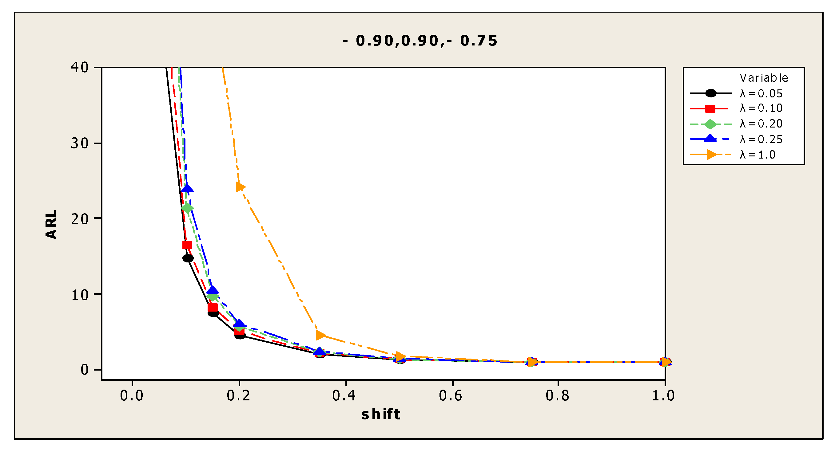
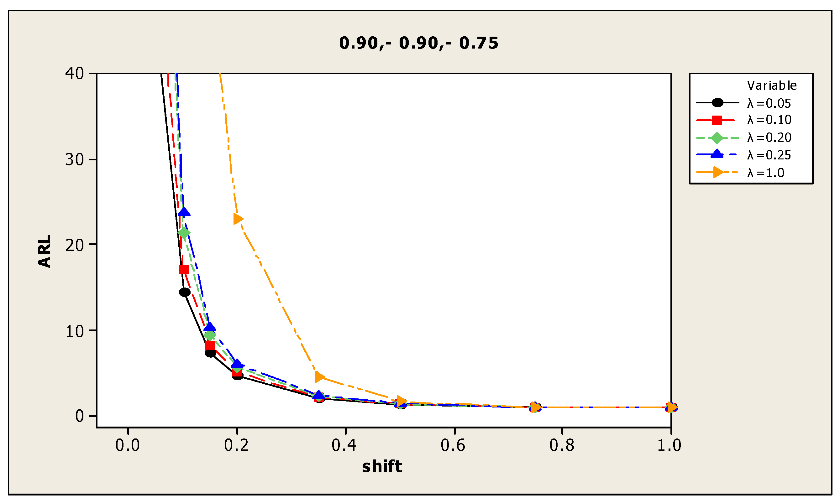
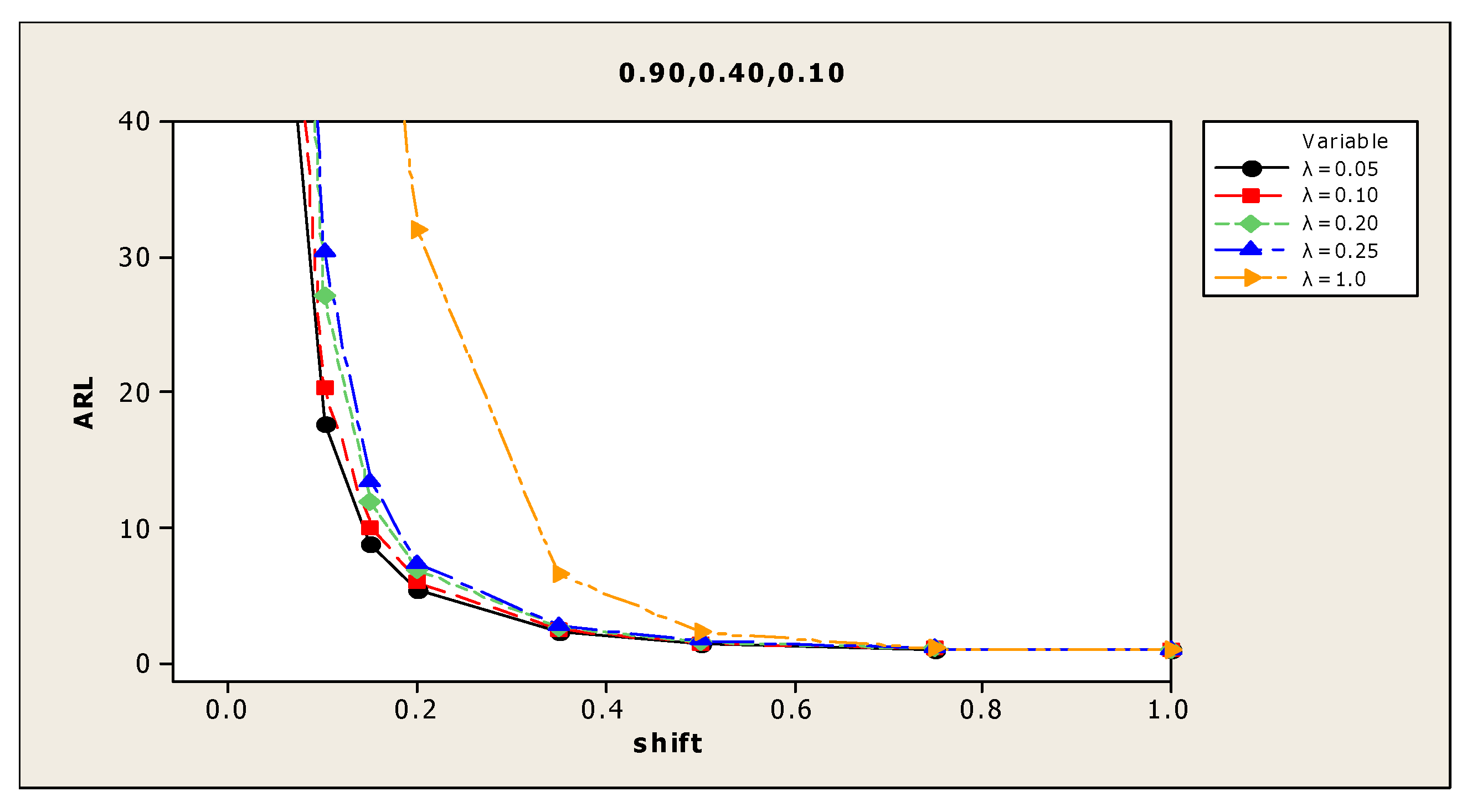
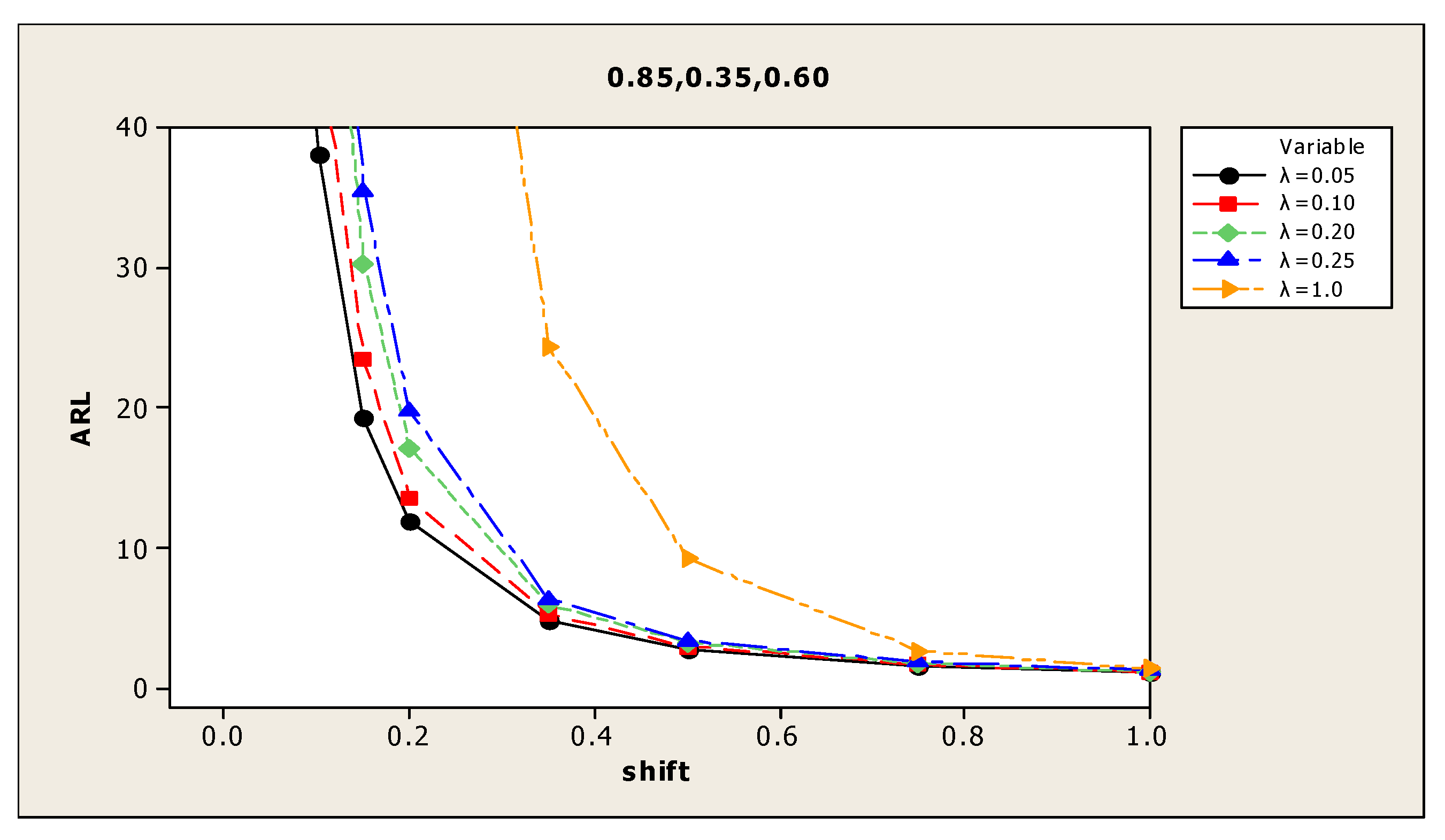
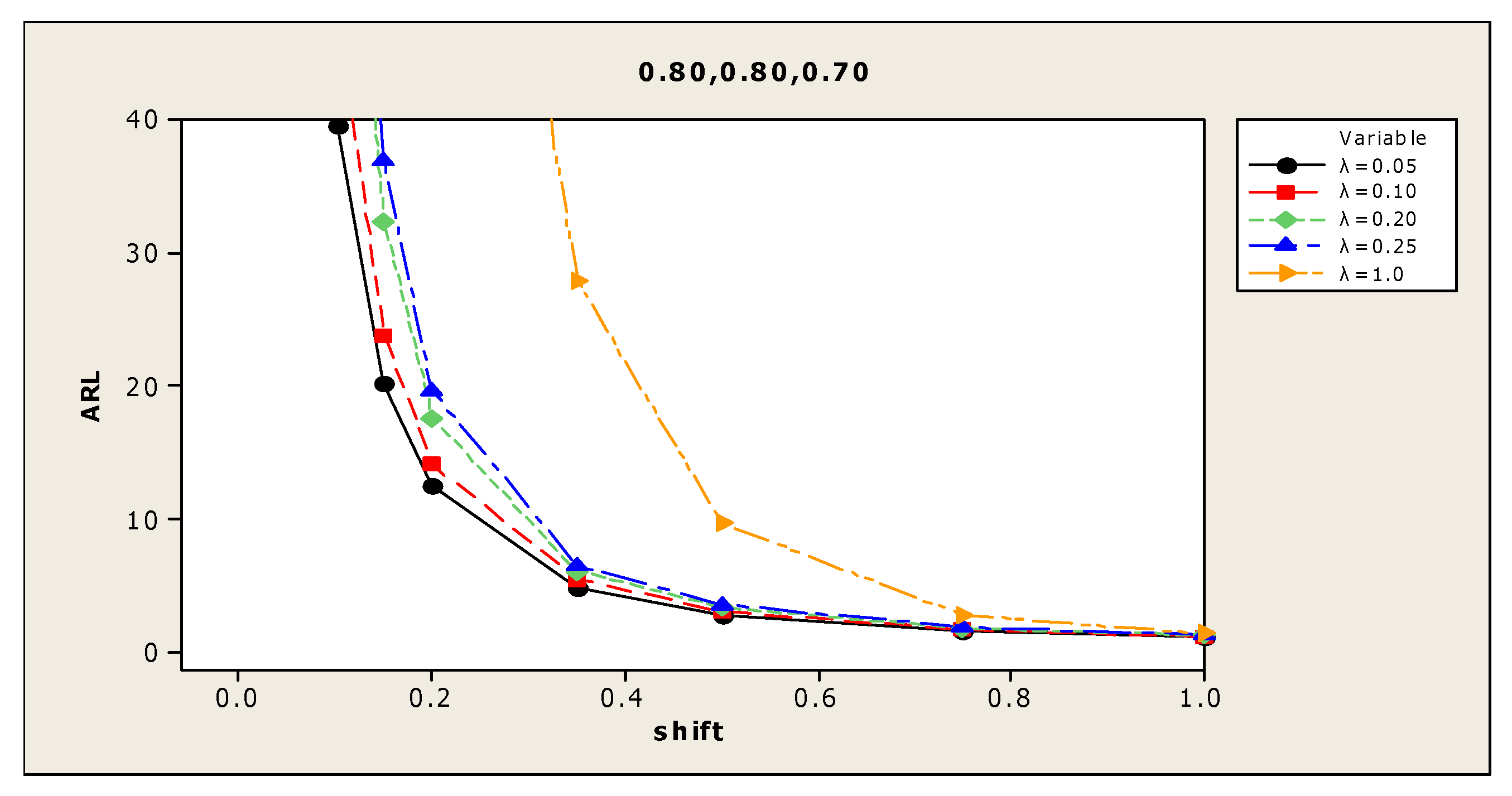
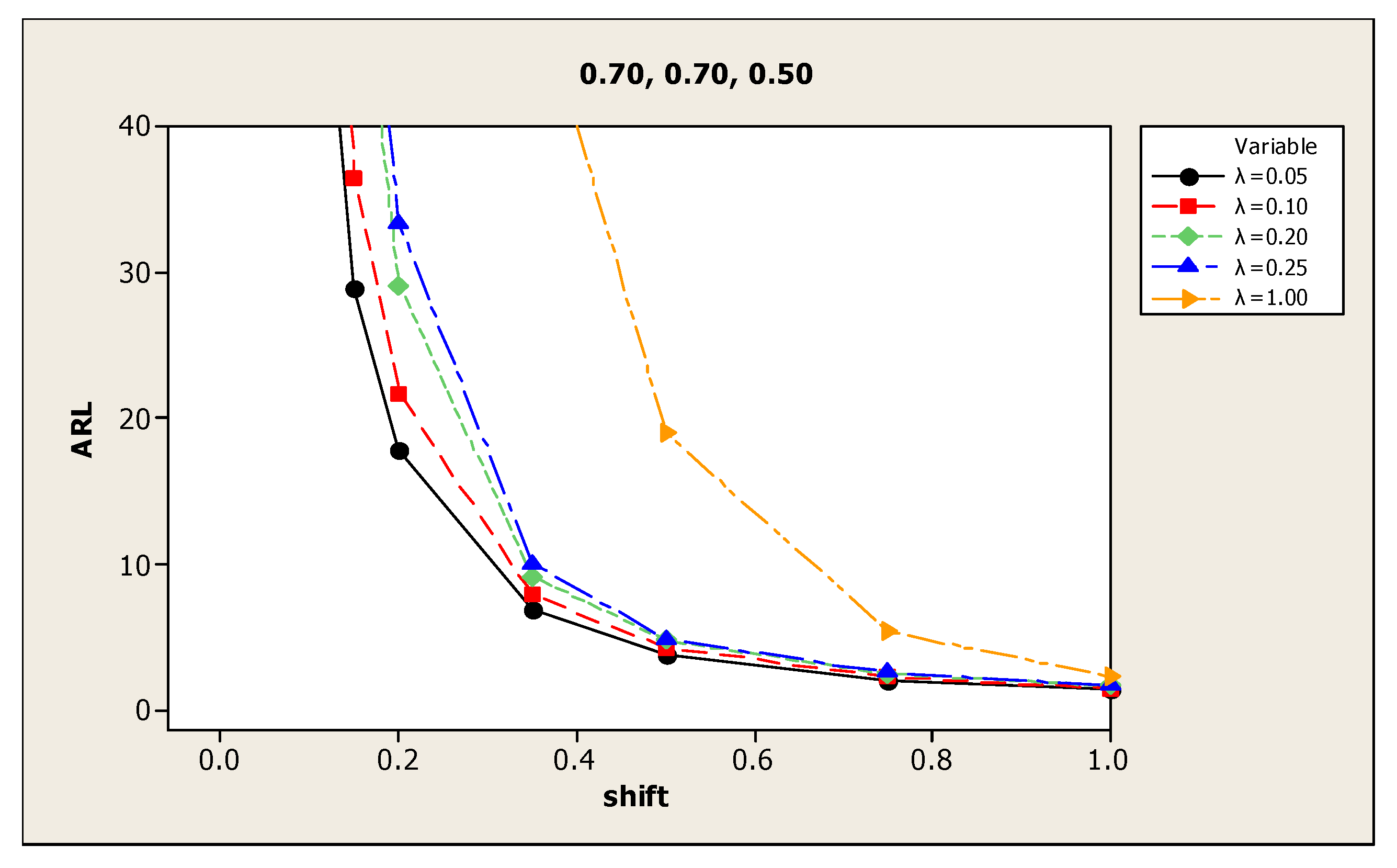
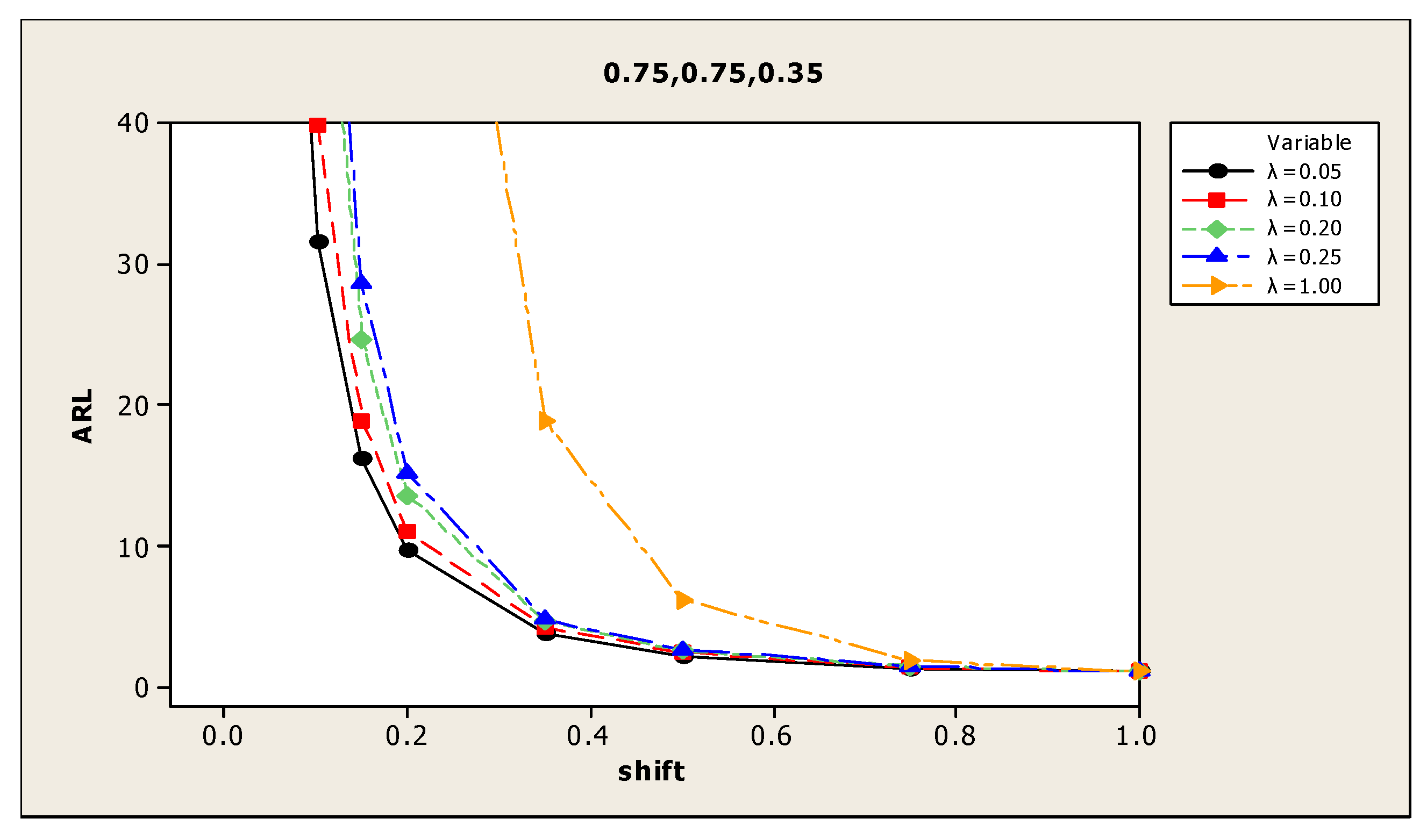
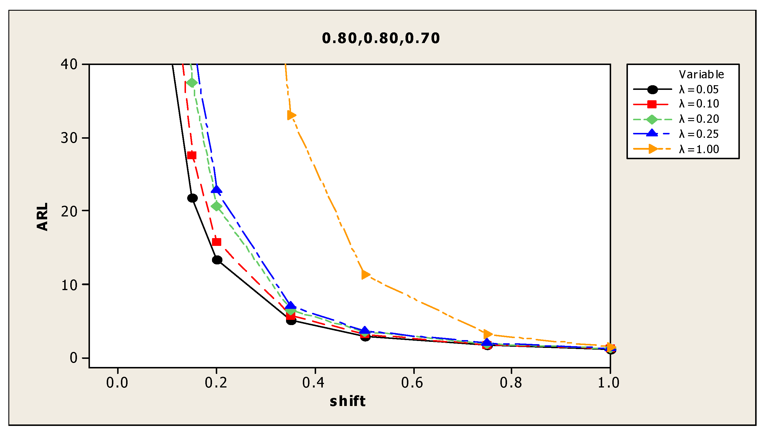
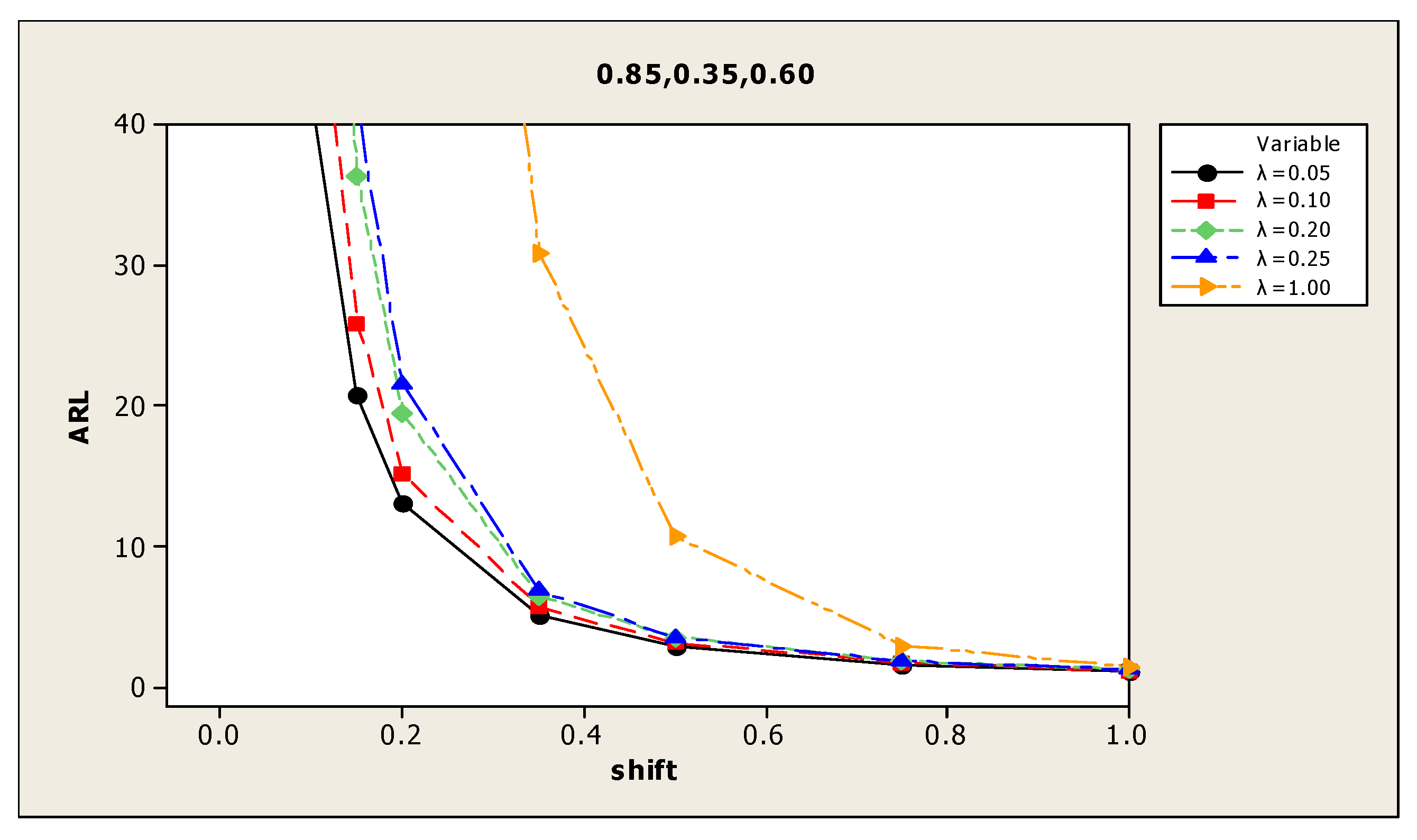
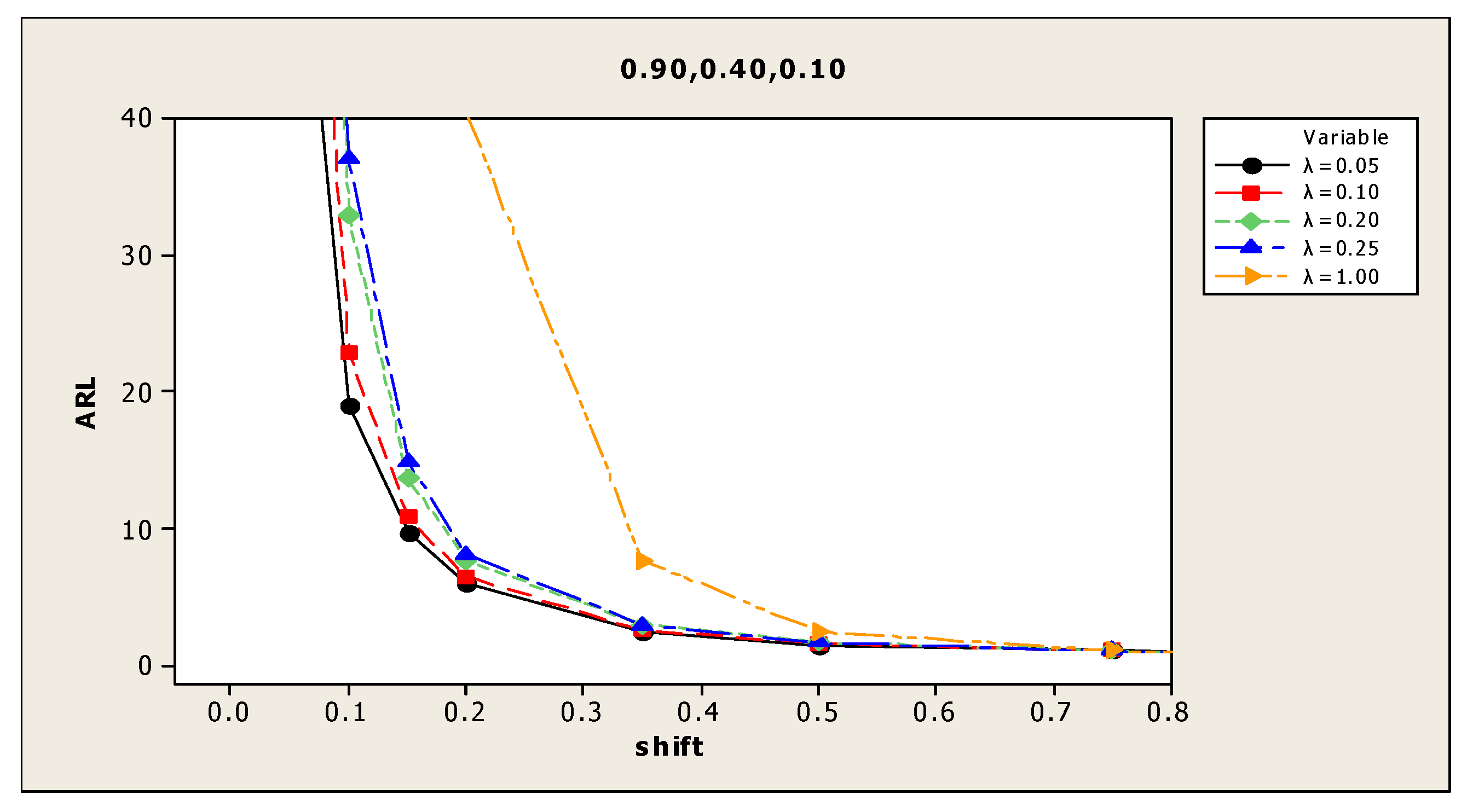
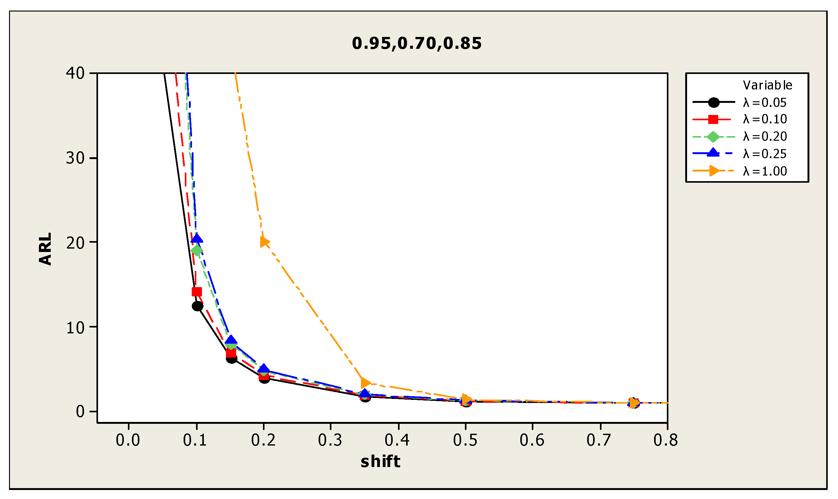
To observe the performance of proposed chart graphically, ARL curves have been represented in the Figure 1, Figure 2, Figure 3, Figure 4, Figure 5, Figure 6, Figure 7, Figure 8, Figure 9, Figure 10, Figure 11, Figure 12, Figure 13 and Figure 14. In the Figure 1, Figure 2, Figure 3, Figure 4, Figure 5, Figure 6 and Figure 7, ARL curves are corresponding to ARL0 = 370 and Figure 8, Figure 9, Figure 10, Figure 11, Figure 12, Figure 13 and Figure 14 are pertaining to ARL0 = 500. In all these Figure 1, Figure 2, Figure 3, Figure 4, Figure 5, Figure 6, Figure 7, Figure 8, Figure 9, Figure 10, Figure 11, Figure 12, Figure 13 and Figure 14, ARL curves corresponding to “λ = 1” represent the performance of existing chart whereas other curves are representing the performance of proposed chart. It is quite clear from the given Figure 1, Figure 2, Figure 3, Figure 4, Figure 5, Figure 6, Figure 7, Figure 8, Figure 9, Figure 10, Figure 11, Figure 12, Figure 13 and Figure 14, that chart performs better when “λ ≠ 1” and moreover, it’s performance improves as the value of “λ” decreases.
The ARLs in the below mentioned tables have been computed by selecting few combinations of correlation coefficients where results can be compared with the performance of the existing chart. It is quite clear that the proposed chart outperforms the existing chart in all the correlation combinations where ARLs have been simulated. It can also be proved that at any scenario of the correlation combination, the proposed chart performs better. Now discussing the proposed chart individually, it is very clear that its performance is highly dependent on the choice value of “λ”. At the smaller values of this parameter, the chart is more sensitive to capture the shifts. As the value of “λ” increases the sensitivity of the chart decreases, so the usefulness of the chart lies in the appropriate selection of “λ”. Another advantage of the chart is that even on correlation coefficients that are not very strong; the chart is quite smart to handle the case.
Following are ARL Curves of the Proposed Charts at few selective correlation combinations. In the given charts the curve corresponding to λ = 1 represents performance of existing chart.

4. Comparison of EWMA-DiD Control Chart with Other Control Charts

In the below mentioned Table 4, ARLs of different commonly used techniques have been compared. It is quite clear from the comparison that X ¯ -chart, CUSUM, and EWMA charts are performing equally for shifts greater than 1, CUSUM and EWMA charts are performing equally for moderate shifts; i.e., 0.5 to 1 (both inclusive) and for the same shift size X ¯ D i D is performing better than CUSUM and EWMA. Therefore, as far as small shifts are concerned, the proposed EWMA-DiD is best in performance. ARLs in the above mentioned table have been computed from tri-variate normal, simulated data with parameters as μ y =   μ u = μ v = 0 and σ y =   σ u = σ v = 1 with ρ y u = 0.8 , ρ y v = 0.8 , ρ u v = 0.7 . The sample size has been taken as n = 3 for the simulated data. The correlations and other information related to auxiliary variables U and V, are applicable for EWMA-DiD and X ¯ D i D control charts, whereas, X ¯ -chart, CUSUM and EWMA charts are using parameters related to variable Y only. In computing the ARLs of the proposed chart, the weighing constant λ assumes values of 0.05, 0.10, 0.20, and 0.25. As the chart takes one variable for quality control monitoring and two as auxiliary variables, there is no need to compare the performance with multivariate charts. This has also been advised by Shabbir and Awan [2].

5. Application of Proposed Chart on Real Data Obtained from Industry

The data were taken from an industry producing Yarn. The variables are related to the Auto cone department, which are RH% (Relative Humidity Percentage), Ambient Temperature in Celsius, and Ambient RH. RH% is very important to maintain in the department because the tensile strength of the yarn as well as the final quality of their end product is highly dependent on it. Their procedures are well standardized to control the defect rate and quality of their product.
They provided around 11,000 observations that were recorded from the actual process and, after the filtration by removing the rows containing missing entries, 10,266 rows were available for the parameter estimation and charting purpose. For parameter estimation, 1000 samples of 1000 size each without replacement were selected assuming that the process is well in control from first 8000 entries and the remaining were kept for charting purpose.
The parameters were computed as follows (Table 5):
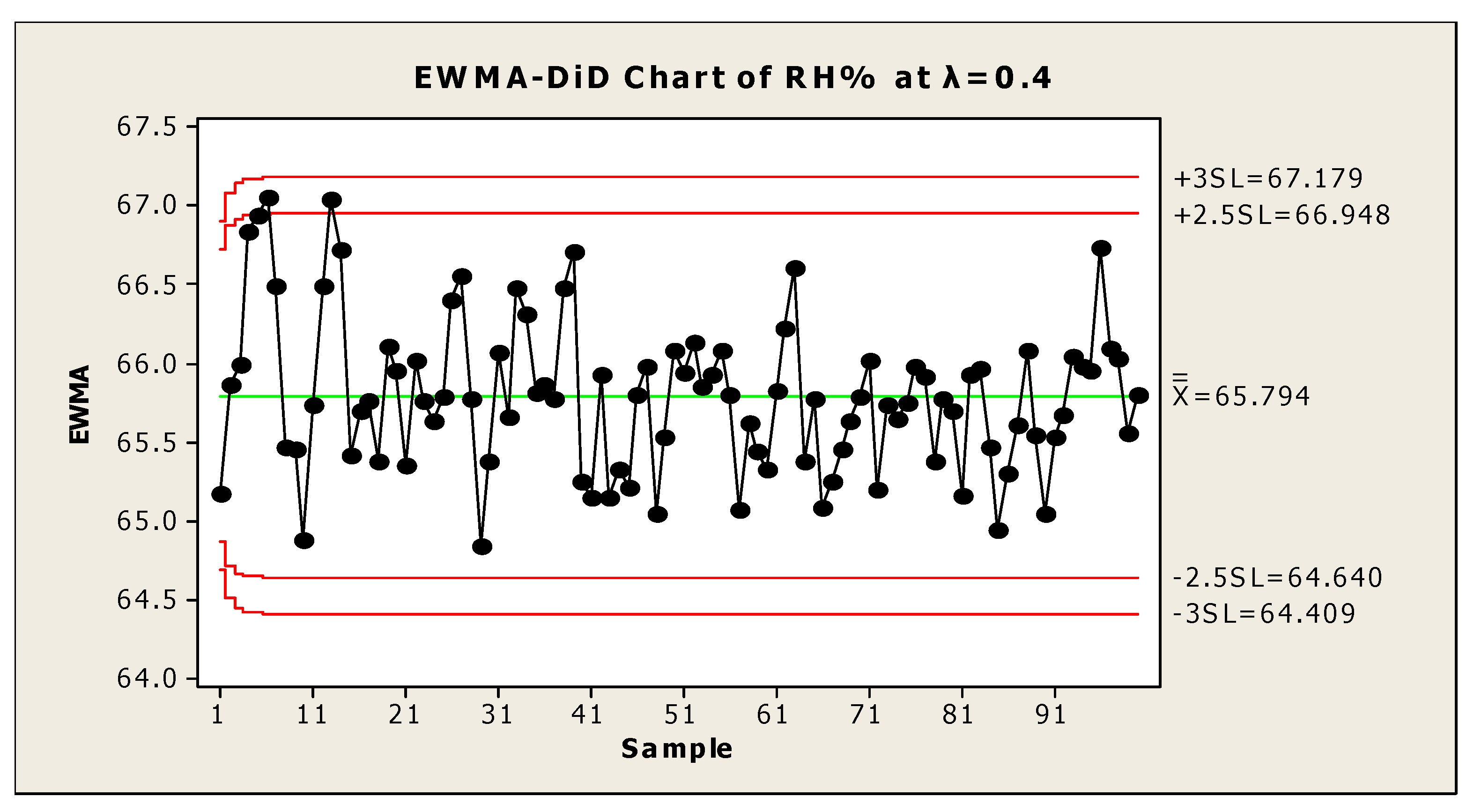
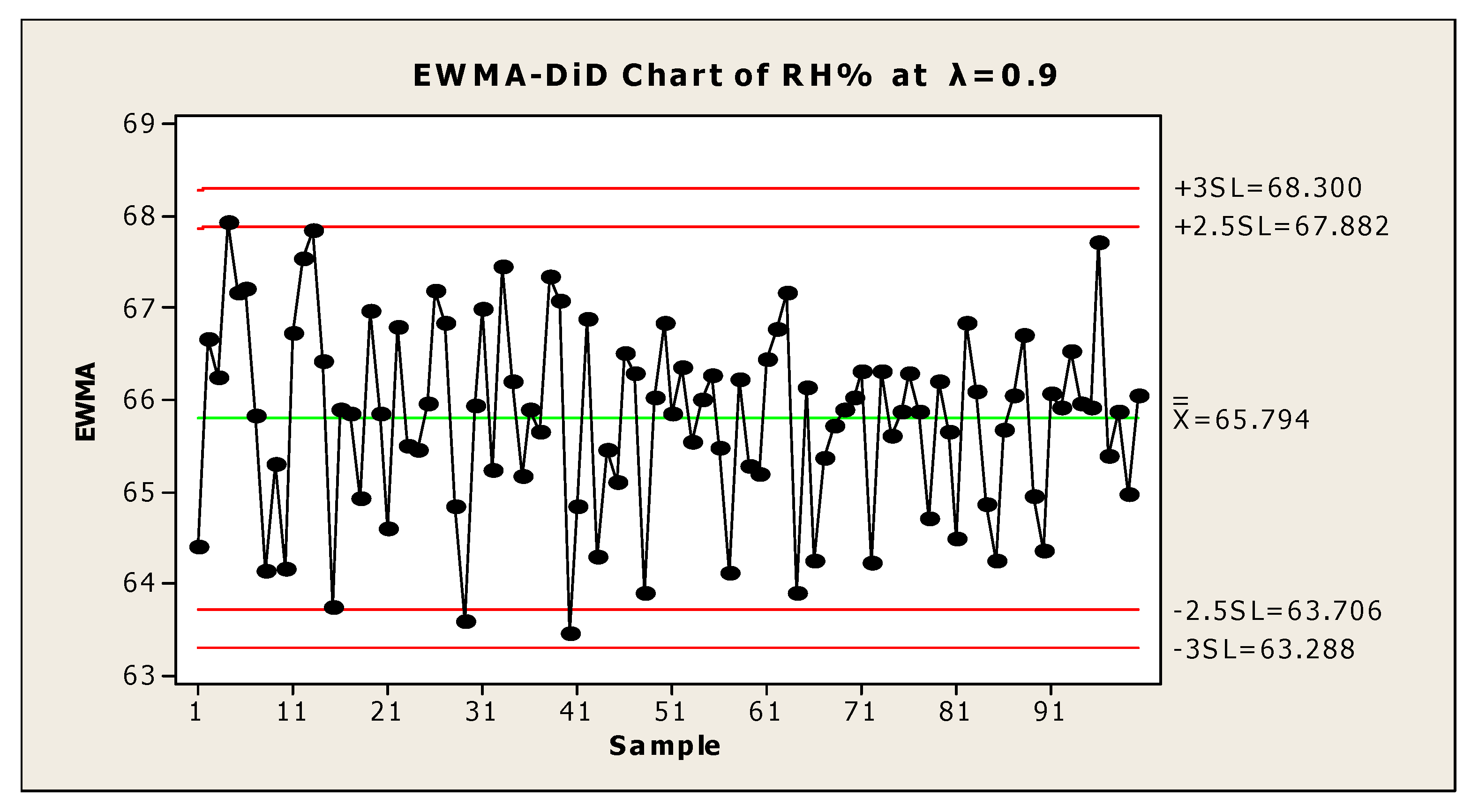
From the data pool kept for charting, 100 subgroups of size 3 each were selected for the construction of the control chart. The charts have been constructed in Figure 15, Figure 16 and Figure 17, selecting different values of λ. The control lines have been drawn at L = 3.00 as Action limits and Warning limits are at L = 2.50.

6. Conclusions

From the application and the simulation results of the proposed chart, we observe that the chart mechanism is very smart in detecting shifts if the main quality concerned variable is strongly correlated with at least one of the auxiliary variables. Otherwise, as the correlation becomes weaker, the performance of the chart becomes less efficient. In case one of the auxiliary variables is uncorrelated, the chart’s efficiency is close to a simple X-bar chart. In the above mentioned application, there are three charts in Figure 15, Figure 16 and Figure 17, from the same data at different values of λ. As the value of λ decreases from 0.5, the weight-age to present value of statistic becomes smaller than previous information. As such the chart shows different behaviors of the process control at varying values of λ. At smaller value of this weighting constant, minor drifts in the process are in pattern; at the higher value of λ the points that are close to upper action limits are highlighted. It is suggested in light of the above mentioned findings, for an in-depth analysis of the process the chart should be assigned different values of λ to listen to the voice of the process.

Author Contributions

Conceptualization, M.A.M., M.A. (Muhammad Azam) and M.A. (Muhammad Aslam); Methodology, M.A.M., M.A. (Muhammad Azam) and M.A. (Muhammad Aslam); Software, M.A.M., M.A. (Muhammad Azam) and M.A. (Muhammad Aslam); Validation, M.A.M., M.A. (Muhammad Azam) and M.A. (Muhammad Aslam); Formal Analysis, M.A. (Muhammad Azam) and M.A. (Muhammad Aslam); Investigation, M.A.M., M.A. (Muhammad Azam) and M.A. (Muhammad Aslam); Writing-Original Draft Preparation, M.A.M; Writing-Review & Editing, M.A.M., M.A. (Muhammad Azam) and M.A. (Muhammad Aslam); Supervision, M.A. (Muhammad Azam) and M.A. (Muhammad Aslam).

Funding

This research received no external funding.

Acknowledgments

The authors are deeply thankful to reviewers and the editor for their valuable suggestions to improve the quality and presentation of this manuscript.

Conflicts of Interest

The authors declare no conflict of interest.

References

  1. Roberts, S.W. Control Chart Tests Based on Geometric Moving Averages. Technometrics 1959, 1, 239–250. [Google Scholar] [CrossRef]
  2. Shabbir, J.; Awan, W.H. An efficient Shewhart-Type control chart to monitor moderate size shifts in the process mean in phase-ii. Qual. Reliab. Eng. Int. 2015, 32, 1597–1619. [Google Scholar] [CrossRef]
  3. Abbas, N.; Riaz, M.; Does, R.J.M.M. Mixed exponentially weighted moving average-cumulative sum charts for process monitoring. Qual. Reliab. Int. 2013, 29, 345–356. [Google Scholar] [CrossRef]
  4. Haq, A. A new hybrid exponentially weighted moving average control chart for monitoring process mean. Qual. Reliab. Eng. Int. 2013, 29, 1015–1025. [Google Scholar] [CrossRef]
  5. Lucas, J.M.; Saccucci, M.S. Exponentially Weighted Moving Average Control Schemes: Properties and Enhancements. Technometrics 1990, 32, 1–12. [Google Scholar] [CrossRef]
  6. Capizzi, G.; Masarotto, G. An adaptive exponentially weighted moving average control chart. Technometrics 2003, 45, 199–207. [Google Scholar] [CrossRef]
  7. Jiang, W.; Shu, L.; Aplet, D.W. Adaptive CUSUM procedures with EWMA-based shift estimators. IIE Trans. 2008, 40, 992–1003. [Google Scholar]
  8. Abbasi, S.A.; Miller, A. On Proper Choice of Variability Control Chart for Normal and Non-Normal Processes; John Wiley & Sons, Ltd.: Hoboken, NJ, USA, 2011. [Google Scholar]
  9. Aslam, M.; Azam, M.; Khan, N.; Jun, C.-H. A mixed control chart to monitor the process. Int. J. Prod. Res. 2015, 53, 4684–4693. [Google Scholar] [CrossRef]
  10. Azam, M.; Aslam, M.; Jun, C.-H. Designing of a hybrid exponentially weighted moving average control chart using repetitive sampling. Int. J. Adv. Manuf. Technol. 2014, 77, 1927–1933. [Google Scholar]
  11. Haq, A.; Brown, J.; Moltchanova, E. A new maximum exponentially weighted moving average control chart for monitoring process mean and dispersion. Qual. Reliab. Eng. Int. 2014. [Google Scholar] [CrossRef]
  12. Haq, A.; Brown, J.; Moltchanova, E.; Al-Omari, A.I. Effect of measurement error on exponentially weighted moving average control charts under ranked set sampling schemes. J. Stat. Comput. Simul. 2014, 85, 1224–1246. [Google Scholar] [CrossRef]
  13. Aslam, M.; Khan, N.; Aldosari, M.S.; Jun, C.-H. Mixed Control Chart Using EWMA Statistics. IEEE Access 2016, 4, 8286–8293. [Google Scholar] [CrossRef]
  14. Ali, R.; Haq, A. A mixed GWMA–CUSUM control chart for monitoring the process mean. Commun. Stat. Theory Methods 2018, 47, 3779–3801. [Google Scholar] [CrossRef]
  15. Sheu, S.H.; Lin, T.C. The generally weighted moving average control chart for detecting small shifts in the process mean. Qual. Eng. 2003, 16, 209–231. [Google Scholar] [CrossRef]
  16. Ajadi, J.O.; Riaz, M. Mixed multivariate EWMACUSUM control charts for an improved process monitoring. Commun. Stat. Theory Methods 2017, 46, 6980–6993. [Google Scholar] [CrossRef]
  17. Riaz, M.; Khaliq, Q.-U.-A.; Gul, S. Mixed Tukey EWMA-CUSUM control chart and its applications. Qual. Technol. Quant. Manag. 2017, 14, 378–411. [Google Scholar] [CrossRef]
  18. Hanif, M.; Hamad, N.; Shahbaz, Q. A modified regression type estimator in survey sampling. World Appl. Sci. J. 2009, 7, 1559–1561. [Google Scholar]
  19. Hamad, N.; Hanif, M.; Haider, N. A regression type estimator with auxiliary variables for two-phase sampling. Open J. Stat. 2013, 3, 74–78. [Google Scholar] [CrossRef]
  20. Awan, W.H.; Shabbir, J. On optimum regression estimator for population mean using two auxiliary variables in simple random sampling. Commun. Stat. Simul. Comput. 2014, 43, 1508–1522. [Google Scholar]
  21. Abbassi, S.A.; Riaz, M. On enhanced control charting for process monitoring. Int. J. Phys. Sci. 2013, 8, 759–775. [Google Scholar]
  22. Zhang, G.X. Cause-selecting control charts—A new type of control charts. QR J. 1985, 12, 221–225. [Google Scholar]
  23. Abbas, N.; Riaz, M.; Does, J.M.M.R. An EWMA-Type control chart for monitoring the process mean using auxiliary information. Commun. Stat. Theory Methods 2014, 43, 3485–3498. [Google Scholar] [CrossRef]
Figure 1. Average run length (ARL) curves when ρ y u = 0.65 , ρ y v = 0.30 ,   ρ u v = 0.50 at above values of λ.
Technologies 06 00069 g001
Figure 2. ARL curves when ρ y u = 0.9 , ρ y v = 0.9 , ρ u v = 0.75 at above values of λ.
Technologies 06 00069 g002
Figure 3. ARL curves when ρ y u = 0.9 , ρ y v = 0.9 , ρ u v = 0.75 at above values of λ.
Technologies 06 00069 g003
Figure 4. ARL curves when ρ y u = 0.9 , ρ y v = 0.9 , ρ u v   = 0.75 at above values of λ.
Technologies 06 00069 g004
Figure 5. ARL curves when ρ y u = 0.9 , ρ y v = 0.4 , ρ u v = 0.1 at above values of λ.
Technologies 06 00069 g005
Figure 6. ARL curves when ρ y u = 0.85 , ρ y v = 0.35 , ρ u v = 0.60 at above values of λ.
Technologies 06 00069 g006
Figure 7. ARL curves when ρ y u = 0.8 , ρ y v = 0.8 , ρ u v = 0.7 at above values of λ.
Technologies 06 00069 g007
Figure 8. ARL curves when ρ y u = 0.7 , ρ y v = 0.7 , ρ u v = 0.5 at above values of λ.
Technologies 06 00069 g008
Figure 9. ARL curves when ρ y u = 0.7 , ρ y v = 0.7 , ρ u v = 0.35 at above values of λ.
Technologies 06 00069 g009
Figure 10. ARL curves when ρ y u = 0.8 , ρ y v = 0.8 , ρ u v = 0.7 at above values of λ.
Technologies 06 00069 g010
Figure 11. ARL curves when ρ y u = 0.85 , ρ y v = 0.35 , ρ u v = 0.60 at above values of λ.
Technologies 06 00069 g011
Figure 12. ARL curves when ρ y u = 0.9 , ρ y v = 0.4 , ρ u v = 0.1 at above values of λ.
Technologies 06 00069 g012
Figure 13. ARL curves when ρ y u = 0.9 , ρ y v = 0.9 , ρ u v   = 0.75 at above values of λ.
Technologies 06 00069 g013
Figure 14. ARL curves when ρ y u = 0.95 , ρ y v = 0.7 , ρ u v = 0.85 at above values of λ.
Technologies 06 00069 g014
Figure 15. EWMA-DiD Chart of RH% at λ = 0.20.
Technologies 06 00069 g015
Figure 16. EWMA-DiD Chart of RH% at λ = 0.40.
Technologies 06 00069 g016
Figure 17. EWMA-DiD Chart of RH% at λ = 0.90.
Technologies 06 00069 g017
Table 1. Percentage relative efficiency of estimators.
Simple MeanRatio EstimatorClassical Regression EstimatorRegression Estimator with Two Auxiliary VariablesEstimator Used in Proposed Chart
100603.37635.08233.3711,620.59
Table 2. ARL0 = 370.
ρ y u , ρ y v ,
ρ u v
Shift(f)λ = 0.05λ = 0.10λ = 0.20λ = 0.25λ = 1.00 ρ y u , ρ y v ,
ρ u v
λ = 0.05λ = 0.10λ = 0.20λ = 0.25λ = 1.00
(1)
0.95,
0.95,
0.85
0.00375.5374.1368.1349.5355.1(7)
0.90,
0.10,
0.52
364.1375.0365.3374.7366.8
0.0518.320.927.732.5130.64.45.05.25.721.7
0.105.66.47.37.634.61.61.71.81.92.8
0.153.03.33.73.711.21.11.11.11.21.2
0.202.02.22.32.34.51.01.01.01.01.0
0.351.11.11.21.21.21.01.01.01.01.0
0.501.01.01.01.01.01.01.01.01.01.0
0.751.01.01.01.01.01.01.01.01.01.0
1.001.01.01.01.01.01.01.01.01.01.0
(2)
0.95,
0.70,
0.85
0.00370.7366.1347.9374.9369.2(8)
0.85,
0.35,
0.60
375.4370.8355.2367.3358.1
0.0536.145.161.272.6215.0109.6146.6179.3186.6316.3
0.1011.113.315.618.485.638.147.465.678.0216.4
0.156.16.67.47.734.119.323.430.335.4139.0
0.203.64.14.54.716.212.013.617.119.890.1
0.351.71.81.91.93.04.85.36.06.424.4
0.501.11.21.21.21.32.83.03.33.49.3
0.751.01.01.01.01.01.61.71.81.92.7
1.001.01.01.01.01.01.21.21.21.31.4
(3)
0.90,
0.90,
0.75
0.00376.0368.0371.6365.6365.5(9)
0.80,
0.80,
0.70
388.4360.1364.0375.0358.9
0.0545.556.682.094.0250.3115.9140.8185.7204.4331.1
0.1014.717.021.324.0111.139.548.769.779.1225.5
0.157.38.49.510.448.520.223.832.336.9148.6
0.204.75.15.76.023.912.514.117.619.693.0
0.351.92.22.32.34.64.95.56.16.527.9
0.501.31.41.41.41.72.83.13.43.69.7
0.751.01.01.01.01.01.61.71.81.92.8
1.001.01.01.01.01.01.21.21.31.31.4
(4)
0.90,
0.40,
0.10
0.00359.7374.7359.2363.6372.3(10)
0.75,
0.75,
0.35
381.2367.8361.0365.1362.7
0.0556.370.497.6113.6265.190.0108.2150.8165.7301.5
0.1017.720.427.230.4124.428.335.349.454.8195.9
0.158.910.111.913.460.414.216.622.225.1106.0
0.205.56.06.97.432.08.910.111.713.566.8
0.352.32.52.72.86.63.54.04.44.515.3
0.501.41.51.61.72.32.12.32.52.65.3
0.751.01.11.11.11.11.31.41.41.41.7
1.001.01.01.01.01.01.01.11.11.11.1
(5)
0.70,
0.70,
0.50
0.00373.0359.8359.0371.0378.5(11)
−0.90,
0.90,
−0.75
370.8373.7373.0357.3357.4
0.05145.3173.3208.6227.1326.746.657.980.794.6239.5
0.1053.668.090.5109.6248.614.816.521.423.9107.0
0.1527.332.544.349.6185.57.58.39.810.549.2
0.2016.519.225.027.4126.34.65.15.76.124.2
0.356.37.18.48.841.42.02.22.32.44.6
0.503.64.04.54.715.51.31.41.41.51.8
0.752.02.22.32.44.61.01.01.01.01.0
1.001.41.51.61.62.11.01.01.01.01.0
(6)
0.65,
0.30,
0.50
0.00369.2382.1359.9359.6367.4(12)
0.90,
−0.90,
−0.75
387.2380.6350.2367.5364.0
0.05188.7225.1257.2274.9350.145.957.283.993.5242.0
0.1077.6100.7130.1146.9297.114.417.121.423.8107.4
0.1540.751.370.680.0237.47.38.39.410.349.4
0.2025.630.742.048.8165.94.75.15.76.123.0
0.3510.211.113.415.468.92.02.22.32.44.6
0.505.56.16.87.231.11.31.41.41.51.7
0.752.93.23.43.79.91.01.01.01.01.0
1.001.92.12.32.34.21.01.01.01.01.0
Table 3. ARL0 = 500.
ρ y u , ρ y v ,
ρ u v
Shift(f)λ = 0.05λ = 0.10λ = 0.20λ = 0.25λ = 1.00 ρ y u , ρ y v ,
ρ u v
λ = 0.05λ = 0.10λ = 0.20λ = 0.25λ = 1.00
(1)
0.95,
0.95,
0.85
0.00508.7490.9521.9478.7489.6(7)
0.90,
0.10,
0.52
499.8478.4508.7491.7490.1
0.0520.023.733.837.8173.94.85.25.86.126.8
0.106.36.87.98.441.31.71.81.92.03.2
0.153.23.63.84.013.11.11.11.21.21.3
0.202.12.32.52.55.01.01.01.01.01.0
0.351.11.11.21.21.31.01.01.01.01.0
0.501.01.01.01.01.01.01.01.01.01.0
0.751.01.01.01.01.01.01.01.01.01.0
1.001.01.01.01.01.01.01.01.01.01.0
(2)
0.95,
0.70,
0.85
0.00506.0478.7508.1485.5484.0(8)
0.85,
0.35,
0.60
487.9479.4515.5502.1485.7
0.0541.054.078.990.5292.9138.9173.8255.2270.1426.6
0.1012.514.119.120.4109.941.355.686.394.9286.3
0.156.47.08.08.443.220.825.936.341.3187.7
0.204.04.34.85.020.113.215.219.521.6119.0
0.351.71.92.02.03.45.15.76.56.930.9
0.501.21.21.31.31.42.93.23.63.610.7
0.751.01.01.01.01.01.61.81.91.93.0
1.001.01.01.01.01.01.21.21.31.31.5
(3)
0.90,
0.90,
0.75
0.00493.9490.7533.6494.9498.0(9)
0.80,
0.80,
0.70
485.0475.5495.2495.2482.5
0.0551.768.8109.3117.9329.9138.6181.2256.7278.6429.6
0.1015.318.525.928.7146.144.060.286.398.2305.5
0.158.09.010.711.661.821.927.637.543.9188.4
0.205.15.66.26.528.713.415.820.722.8118.9
0.352.12.32.52.55.45.25.86.57.133.1
0.501.31.41.51.51.93.03.23.63.711.3
0.751.01.01.01.01.01.71.81.92.03.2
1.001.01.01.01.01.01.21.31.31.31.5
(4)
0.90,
0.40,
0.10
0.00461.8480.6499.1489.2481.8(10)
0.75,
0.75,
0.35
487.0486.5501.6487.5488.0
0.0565.086.5127.9137.1348.7100.8135.3193.9222.5424.0
0.1019.122.932.937.0173.431.639.960.267.7246.1
0.159.710.913.714.980.616.218.924.628.6140.5
0.206.16.57.78.140.49.711.013.615.278.6
0.352.52.63.03.07.73.94.24.74.818.9
0.501.51.61.71.72.52.22.52.62.76.2
0.751.11.11.11.11.11.31.41.51.51.9
1.001.01.01.01.01.01.11.11.11.11.1
(5)
0.70,
0.70,
0.50
0.00488.9498.3520.7495.9507.6(11)
−0.90,
0.90,
−0.75
484.4476.7505.3508.4490.3
0.05174.5222.7311.6323.5417.851.367.9102.5116.4330.6
0.1059.380.2119.4138.2346.815.818.624.428.3137.9
0.1529.036.455.763.2237.68.09.010.711.660.6
0.2017.821.729.133.3155.24.95.46.36.429.1
0.357.07.99.210.150.72.12.32.52.55.2
0.503.94.34.84.919.01.31.41.51.51.9
0.752.12.32.52.65.41.01.01.01.01.1
1.001.51.51.71.72.31.01.01.01.01.0
(6)
0.65,
0.30,
0.50
0.00489.9507.5506.1486.0493.2(12)
0.90,
−0.90,
−0.75
488.0478.9516.1477.2492.1
0.05236.4290.7358.0393.0471.053.268.6105.7117.2337.2
0.1092.0120.9176.3197.8386.316.117.825.327.8136.4
0.1546.261.989.3104.0311.47.98.910.811.659.1
0.2028.633.853.557.9228.44.95.56.36.528.8
0.3510.912.015.416.692.52.12.32.52.55.1
0.505.96.77.97.939.71.31.41.51.51.9
0.753.03.43.73.811.61.01.01.01.01.1
1.002.02.22.42.44.81.01.01.01.01.0
Table 4. Comparison of different control charts.
Shift X ¯ Chart CUSUM k = 0.5EWMA ChartEWMA-DiD X ¯ D i D - Chart
λ = 0.05λ = 0.1λ = 0.2λ = 0.25λ = 0.5
0.00500.5502.8499.9499.8499.6500.0500.5495.8490.1
0.25241.252.435.540.555.864.8116.9<13.078.1
0.5076.213.413.612.713.714.925.1<3.711.3
0.7527.37.18.37.36.86.99.1<2.03.2
1.0011.54.86.15.14.54.44.8<1.31.5
1.503.23.04.03.32.82.62.41.01.0
2.001.52.33.12.52.12.01.61.01.0
2.501.11.92.52.11.71.61.21.01.0
3.001.01.62.11.91.41.31.01.01.0
Table 5. Process parameters.
VariablesParametersVariable Type
RH% μ y = 65.794 σ y = 2.0266 ρ y u =   0.3498 Quality Concern
Amb TC μ u = 26.403 σ u = 3.3591 ρ y v =   0.3374 Auxiliary Information
Amb RH μ v = 69.6995 σ v = 9.3185 ρ u v =   0.6688