3D Localization of Near-Field Sources with Symmetric Enhanced Nested Arrays

Abstract

Sparse arrays can effectively reduce antenna cost and implementation complexity. However, most existing research in sparse array design mainly focuses on far-field scenarios, which cannot be directly applied to near-field (NF) source localization, where the delay term and source incident parameters exhibit a nonlinear relationship. In this paper, employing a symmetric enhanced nested array, a high-precision underdetermined three-dimensional (3D) NF localization method is proposed. Firstly, the symmetry of the array and the fourth-order cumulant are utilized to construct the equivalent virtual far-field (FF) received data. Then, a gridless, sparse, and parametric approach combined with an l₁-singular value decomposition-based pairing procedure is employed to obtain estimates of two paired angles. Finally, a one-dimensional (1D) spectral estimator is applied to obtain the estimate of the range parameter. By analyzing the virtual aperture, the optimal parameter configuration for a given number of elements is obtained. As shown by simulation results, the proposed method can handle underdetermined estimation. Compared with the other algorithms, the proposed algorithm achieves significant improvements in both angular and distance accuracy, with enhancements of 65% and 61.7%, respectively.

1. Introduction

Direction of arrival (DOA) estimation and source localization are key research topics in array signal processing and have many applications in wireless communications, radar, and sonar [1,2,3,4,5]. Recently, there has been an increasing interest in applications related to near-field (NF) source localization, such as indoor positioning and autonomous driving [6,7], and many far-field (FF) source localization (known as DOA estimation) algorithms have been adapted for NF localization. By exploiting the symmetric uniform linear arrays (ULAs) to eliminate the quadratic term about range information, the conventional method for DOA estimation of FF sources, such as MUSIC-like methods [8,9], generalized ESPRIT methods [10,11], and gridless sparse methods [12,13], is extended to the NF case, achieving considerable estimation performance. However, compared with sparse arrays [14,15,16], traditional ULAs exhibit poor performance since their degrees of freedom (DOFs) are quite limited, and they fail in DOA estimation in the underdetermined scenario and also require more physical sensors for the same estimation accuracy.

A sparse array is a kind of sensor array with a physically non-uniform distribution, and its element positions are specially designed. Common sparse arrays include the minimum redundant array (MRA) [17], the coprime array (CPA) [18], and the nested array (NA) [19], followed by their evolving arrays [20,21,22,23,24,25,26,27]. Moreover, most existing NF source localization algorithms do not fully utilize the spatial-temporal information of the received data, which limits the potential for further improvement in estimation performance.

Compared with ULA-based NF localization algorithms [8,28,29,30], non-uniform linear arrays (NLA) with associated algorithms [31,32,33,34,35] have more DOFs and can perform effective underdetermined estimation. In [31], a mixed NF and FF source localization scheme based on symmetric double nested arrays is proposed by applying oblique projection and spatial smoothing MUSIC to estimate angle and range parameters. In [32], a hybrid source localization method based on generalized symmetric sparse linear arrays and second-order statistics is proposed. The atomic norm is introduced into the NF source localization algorithm based on sparse arrays. In [33], an NF source localization estimation algorithm based on coprime arrays is proposed by establishing an off-grid model containing only angle parameters to estimate 1D angles iteratively. As deep learning technology continues to mature, reference [34] utilizes the geometric structure of symmetric nested arrays to apply convolutional neural networks (CNNs) for the classification and localization of mixed sources in both near and far fields. Subsequently, in [35], a new symmetric shifted coprime array is proposed, which obtains estimated angle and range through spatial smoothing of the virtual received data. Compared with traditional sparse arrays, this new sparse configuration can provide more consecutive virtual segments and higher DOFs.

Compared with the 2D parameter estimation (azimuth and range) mentioned in [8,28,29,30,31,32,33,34,35], three-dimensional (3D) (azimuth, elevation, and distance) parameter estimation is more relevant to practical applications. In the 3D case, several notable studies utilizing uniform cross arrays have been reported [36,37,38]. As for non-uniform arrays, apart from the 3D NF localization method based on symmetric non-uniform cross arrays [39], research results on 3D NF source localization using NLAs are rather limited, especially in underdetermined situations where the number of sources is greater than the number of array elements.

To fill this gap, in this work, a 3D NF parameter estimation method based on a symmetric enhanced nested array (SENA) is proposed. We firstly utilize the spatial-temporal information of the received signals with fourth-order cumulant (FOC) calculations, providing increased DOFs; then, a gridless sparse and parametric approach (SPA) [40], combined with an l₁-SVD-based pairing procedure, is employed to obtain estimates for two paired angles; finally, a 1D spectral estimator is used for range estimation. The main contributions of this paper are as follows:

•

A SENA array is proposed, which unfolds the nested array and introduces central symmetry, facilitating the elimination nonlinear range-related information inherent in the phase component of the steering matrix for NF signals. An analysis of the SENA array’s properties is provided, followed by a proposal of the optimal virtual array parameter configuration for the proposed SENA array.

•

The FOC calculation is applied to the SENA array’s output, which is vectorized to expand the virtual array aperture, enhancing the parameter estimation performance. Simulation results demonstrate the proposed algorithm’s superiority in parameter estimation accuracy and its abilities in underdetermined and mixed source estimation.

The organization of this paper is as follows: Section 2 provides an introduction to the signal model and array structure. Section 3 describes the content of the algorithm, followed by the total elements of the virtual array, as well as the design optimization of the virtual aperture and complexity analyses in Section 4. Section 5 demonstrates the effectiveness of the proposed algorithm through a series of simulations. Finally, Section 6 concludes with a synopsis.

Notations: Matrices and vectors are denoted by boldfaced capital letters and lower-case letters, respectively. ${(·)}^T$, ${(·)}^{\ast }$, ${(·)}^H$ respectively represent transpose, conjugate, and conjugate transpose. The symbols $E\left\{·\right\}$ and $∥·∥$ represent expectation and norm, respectively. $tr\left(·\right)$ returns the sum of diagonal elements of the corresponding matrix while $vec\left(·\right)$ is the vectorization operation.

2. Signal Model

The symmetric enhanced nested array shown in Figure 1 consists of two subarrays located on the x-axis and y-axis, respectively. The structures of the two subarrays are the same, and both are symmetric about the origin. Among them, each sparse array consists of three parts: a dense subarray, a sparse subarray, and an isolated subarray. The dense subarray referred to as subarray 1 is located at the center of the array, and the position set of the subarray 1 is represented as ${\mathbb{L}}_1=\left\{m_{1}d,1-M_1⩽m_1⩽M_1-1\right\}$, where d is the element spacing unit, and $M_1$ represents the number of subarrays on the positive half axis of subarray 1. The two sparse subarrays are located on the positive and negative axes on both sides of the origin, where the positive segment, denoted as subarray 2 is ${\mathbb{L}}_2=\left\{\left(D{m}_2-1\right)d,1⩽m_2⩽M_2\right\}$ with $D=2M_1$ and $M_2$ representing the number of elements in subarray 2. Using ${\mathbb{L}}_3$ and $M_3$ to represent the position set and number of elements in subarray 3 located on the negative half axis, respectively, we have ${\mathbb{L}}_3=-{\mathbb{L}}_2$ and $M_3=M_2$. The two isolated subarrays are located at both ends of the array, namely subarray 4 and subarray 5. The element position of subarray 4 located on the positive axis is ${\mathbb{L}}_4=\left\{{\mathbb{L}}_4|{\mathbb{L}}_4=\left[D\left(M_2+1\right)+M_1-2\right]d\right\}$, and the number of elements is 1. ${\mathbb{L}}_5$ represents the element positions of subarray 5, and ${\mathbb{L}}_5=-{\mathbb{L}}_4$. Finally, the whole set of array element positions is the union of five subarray position sets, namely $\mathbb{L}={\mathbb{L}}_1\cup {\mathbb{L}}_2\cup {\mathbb{L}}_3\cup {\mathbb{L}}_4\cup {\mathbb{L}}_5$. The total number of elements in a single axis is the sum of the element numbers in five subarrays, denoted as $M_x=M_y=2M_1+2M_2+1$, where $M_x$ and $M_y$ represent the total number of elements on the x and y axes, respectively. The total number of elements in the considered cross array is $M=M_x+M_y-1=4M_1+4M_2+1$.

Assume that there are K narrowband NF sources impinging on the array shown in Figure 1, where the 2D angles of the k-th source relative to the x-axis and y-axis are represented as ${\alpha }_k$ and ${\beta }_k$, respectively, and the range measured from the origin is $r_k$. The received signals of the $m_x$-th element on the x-axis and the $m_y$-th element on the y-axis at time t can be represented as

$$\begin{array}{c}x\left(m_x,t\right)=\sum _{k=1}^K{s}_k\left(t\right)e^{-j{\tau }_{m_x}\left(k\right)}+n_{m_x}\left(t\right)\hfill \\ y\left(m_y,t\right)=\sum _{k=1}^K{s}_k\left(t\right)e^{-j{\tau }_{m_y}\left(k\right)}+n_{m_y}\left(t\right)\hfill \end{array}$$

(1)

where $m_x\in \mathbb{L}$ and $m_y\in \mathbb{L}$ represent the index of the array element position, $s_k\left(t\right)$ is the k-th incident signal, $n_{m_y}\left(t\right)$ and $n_{m_x}\left(t\right)$ are the additive white Gaussian noise at the two corresponding subarrays, and ${\tau }_{m_x}\left(k\right)$ and ${\tau }_{m_y}\left(k\right)$ respectively represent the k-th incident signal’s phase difference from the reference element to the $m_x$-th element on the x-axis and the $m_y$-th element on the y-axis, respectively. According to Taylor’s approximation, (1) can be approximated as

$$\begin{array}{c}x\left(m_x,t\right)=\sum _{k=1}^K{s}_k\left(t\right)e^{-j\left({\omega }_{xk}{m}_x+{\varphi }_{xk}{m_x}^2\right)}+n_{m_x}\left(t\right)\hfill \\ y\left(m_y,t\right)=\sum _{k=1}^K{s}_k\left(t\right)e^{-j\left({\omega }_{yk}{m}_y+{\varphi }_{yk}{m_y}^2\right)}+n_{m_y}\left(t\right)\hfill \end{array}$$

(2)

where ${\omega }_{xk},{\omega }_{yk},{\varphi }_{xk}$ and ${\varphi }_{yk}$ are denoted as

$$\begin{array}{c}{\omega }_{xk}=-{\displaystyle \frac{2\pi cos\left({\alpha }_k\right)}{\lambda }},{\varphi }_{xk}={\displaystyle \frac{\pi {sin}^2\left({\alpha }_k\right)}{\lambda r_k}}\hfill \\ {\omega }_{yk}=-{\displaystyle \frac{2\pi cos\left({\beta }_k\right)}{\lambda }},{\varphi }_{yk}={\displaystyle \frac{\pi {sin}^2\left({\beta }_k\right)}{\lambda r_k}}\hfill \end{array}$$

(3)

3. Proposed Algorithm

3.1. Construction of Virtual FF Data

Based on the FOC of the observed data, a virtual FF co-array can be constructed, which has a larger array aperture and more DOFs than the physical array, resulting in improved parameter estimation accuracy.

With the definition and properties of FOC, we have

$$\begin{array}{cc}\hfill {\mathbf{C}}_x\left(m,n,\tau \right)& =cum\left\{\mathbf{x}\left(m,t+\tau \right),{\mathbf{x}}^{\ast }\left(-m,t\right),\mathbf{x}\left(-n,t+\tau \right),{\mathbf{x}}^{\ast }\left(n,t\right)\right\}\hfill \\ \hfill & =\sum _{k=1}^K{e}^{-j2\left(m-n\right){\omega }_{xk}}{c}_{sk}\left(\tau \right)\hfill \end{array}$$

(4)

$$\begin{array}{cc}\hfill {\mathbf{C}}_y\left(m,n,\tau \right)& =cum\left\{\mathbf{y}\left(m,t+\tau \right),{\mathbf{y}}^{\ast }\left(-m,t\right),\mathbf{y}\left(-n,t+\tau \right),{\mathbf{y}}^{\ast }\left(n,t\right)\right\}\hfill \\ \hfill & =\sum _{k=1}^K{e}^{-j2\left(m-n\right){\omega }_{yk}}{c}_{sk}\left(\tau \right)\hfill \end{array}$$

(5)

where $m\in \mathbb{L}$ and $n\in \mathbb{L}$ represent the element position index, $\tau$ is the delay, and $c_{sk}\left(\tau \right)=cum\left(s_k\left(t+\tau \right),s_k^{\ast }\left(t\right),s_k\left(t+\tau \right),s_k^{\ast }\left(t\right)\right)$ is the FOC of the k-th signal at delay $\tau$. For each delay, vectorizing ${\mathbf{C}}_x$ and ${\mathbf{C}}_y$ separately yields

$$\begin{array}{c}{\mathbf{c}}_x\left(\tau \right)=vec\left({\mathbf{C}}_x\left(:,:,\tau \right)\right)=\mathbf{B}\left({\omega }_{xk}\right){\mathbf{c}}_s\left(\tau \right)\hfill \\ {\mathbf{c}}_y\left(\tau \right)=vec\left({\mathbf{C}}_y\left(:,:,\tau \right)\right)=\mathbf{B}\left({\omega }_{yk}\right){\mathbf{c}}_s\left(\tau \right)\hfill \end{array}$$

(6)

where ${\mathbf{c}}_s\left(\tau \right)={\left[c_{s1}\left(\tau \right),c_{s2}\left(\tau \right),\dots ,c_{sK}\left(\tau \right)\right]}^T$. ${\mathbf{c}}_x\left(\tau \right)$ and ${\mathbf{c}}_y\left(\tau \right)$ are the virtual received data related to subarrays on x and y axis, respectively, $\mathbf{B}\left({\omega }_{xk}\right)=[{\mathbf{b}}_1\left({\omega }_{x1}\right),{\mathbf{b}}_2\left({\omega }_{x2}\right),\cdots ,{\mathbf{b}}_k\left({\omega }_{xk}\right)]$, where ${\mathbf{b}}_k\left({\omega }_{xk}\right)={\overline{\mathbf{b}}}_k\left({\omega }_{xk}\right)\otimes {\overline{\mathbf{b}}}_k\left({\omega }_{xk}\right)$, ${\overline{\mathbf{b}}}_k\left({\omega }_{xk}\right)=\left[e^{-j2{\mathbb{L}}_5{\omega }_{xk}},\cdots ,e^{j2{\omega }_{xk}}, 1, e^{-j2{\omega }_{xk}},\cdots ,\right.$ ${\left.e^{-j2{\mathbb{L}}_4{\omega }_{xk}}\right]}^{\mathrm{T}}$. Similarly, $\mathbf{B}\left({\omega }_{yk}\right)$ follows the same form. Obviously, the virtual array element positions of the x-axis and y-axis are the sets of difference co-array (DCA) of the physical array. Due to the presence of repeated elements in the two DCA sets, it is necessary to remove the redundancy and then rearrange the two sets of virtual received data according to the order of virtual array element positions, which can be represented as

$$\begin{array}{c}{\tilde{\mathbf{c}}}_x\left(\tau \right)=\tilde{\mathbf{B}}\left({\omega }_{xk}\right){\mathbf{c}}_s\left(\tau \right)\hfill \\ {\tilde{\mathbf{c}}}_y\left(\tau \right)=\tilde{\mathbf{B}}\left({\omega }_{yk}\right){\mathbf{c}}_s\left(\tau \right)\hfill \end{array}$$

(7)

By uniform sampling of the delay $\tau$ in $\tau =T_s,2T_s,\dots L{T}_s$, L pseudo snapshots of the virtual received data are obtained, which can be combined and denoted as

$$\begin{array}{cc}\hfill {\tilde{\mathbf{C}}}_x& =\left[{\tilde{\mathbf{c}}}_x\left(T_s\right),{\tilde{\mathbf{c}}}_x\left(2T_s\right),\dots ,{\tilde{\mathbf{c}}}_x\left(L{T}_s\right)\right]\hfill \\ \hfill & =\tilde{\mathbf{B}}\left({\omega }_{xk}\right){\mathbf{C}}_s\hfill \\ \hfill {\tilde{\mathbf{C}}}_y& =\left[{\tilde{\mathbf{c}}}_y\left(T_s\right),{\tilde{\mathbf{c}}}_y\left(2T_s\right),\dots ,{\tilde{\mathbf{c}}}_y\left(L{T}_s\right)\right]\hfill \\ \hfill & =\tilde{\mathbf{B}}\left({\omega }_{yk}\right){\mathbf{C}}_s\hfill \end{array}$$

(8)

Compared with the original array data, the number of virtual array elements constructed in this way has been significantly increased, and the range parameters are no longer included, which facilitates the subsequent estimation process.

3.2. 2D Angle Estimation

In this section, the virtual FF data constructed from the subarrays are used to separately estimate 2D angles ${\alpha }_k$ and ${\beta }_k$. Since holes exist in the virtual arrays, the angle parameters of interest are estimated with SPA [40], which is a gridless method. To begin with, let ${\mathbf{B}}_{\Sigma }$ denote the manifold matrix of the DCA of the virtual array on the x-axis and y-axis, which behaves like the manifold matrix of a ULA. Then, the relationship between $\tilde{\mathbf{B}}$ and ${\mathbf{B}}_{\Sigma }$ can be written as

$$\tilde{\mathbf{B}}=\mathbf{\Gamma }{\mathbf{B}}_{\Sigma }$$

(9)

where $\mathbf{\Gamma }$ is a $P\times Q$ matrix, P is the number of elements in the virtual array including repetitions, and Q is the number of elements in the corresponding ULA.

The virtual received data ${\tilde{\mathbf{C}}}_x$ and ${\tilde{\mathbf{C}}}_y$ are collectively denoted as $\tilde{\mathbf{C}}$, and then the virtual covariance matrix can be expressed as

$$\begin{array}{cc}\hfill \mathbf{R}& =E\left\{\tilde{\mathbf{C}}{\tilde{\mathbf{C}}}^H\right\}\hfill \\ \hfill & =\tilde{\mathbf{B}}{\mathbf{R}}_s{\tilde{\mathbf{B}}}^H\hfill \\ \hfill & =\mathbf{\Gamma }{\mathbf{B}}_{\Sigma }{\mathbf{R}}_s{{\mathbf{B}}_{\Sigma }}^H{\mathbf{\Gamma }}^H\hfill \end{array}$$

(10)

where ${\mathbf{R}}_s$ represents the covariance matrix of the virtual incident signal, and ${\mathbf{R}}_{\Sigma }={\mathbf{B}}_{\Sigma }{\mathbf{R}}_s{\mathbf{B}}_{\Sigma }^H$. As ${\mathbf{B}}_{\Sigma }$ is a Vandermonde matrix, ${\mathbf{R}}_{\Sigma }$ is a Toeplitz matrix with ${\mathbf{R}}_{\Sigma }=\mathbf{T}\left(\mathbf{u}\right)$ as follows:

$$\begin{array}{c}\hfill \mathbf{T}\left(\mathbf{u}\right)=\left[\begin{array}{cccc}{u}_1& u_2& \dots & u_Q\\ u_2^{\ast }& u_1& \dots & u_{Q-1}\\ ⋮& ⋮& \ddots & ⋮\\ u_Q^{\ast }& u_{Q-1}^{\ast }& \dots & u_1\end{array}\right]\end{array}$$

(11)

where $\mathbf{u}$ represents the horizontal quantity in $\mathbf{T}\left(\mathbf{u}\right)$. However, in practice, due to a limited number of snapshots, the covariance matrix is generally replaced by the sample covariance matrix:

$$\begin{array}{c}\hfill \tilde{\mathbf{R}}={\displaystyle \frac{1}{L}}\tilde{\mathbf{C}}{\tilde{\mathbf{C}}}^H\end{array}$$

(12)

Then, SPA is applied to recover the matrix $\mathbf{T}\left(\mathbf{u}\right)$. Since the sample covariance matrix $\tilde{\mathbf{R}}$ is nonsingular, the optimization is formulated as follows:

$$\begin{array}{c}\underset{\mathbf{W},\mathbf{u}}{min}tr\left(\mathbf{W}\right)+tr\left({\tilde{\mathbf{R}}}^{-1}\mathbf{R}\right)\hfill \\ subject\mathrm{to}\left[\begin{array}{ccc}\mathbf{W}& {\tilde{\mathbf{R}}}^{{\displaystyle \frac{\mathbf{1}}{\mathbf{2}}}}& \\ {\tilde{\mathbf{R}}}^{{\displaystyle \frac{\mathbf{1}}{\mathbf{2}}}}& \mathbf{R}& \\ & & \mathbf{T}\left(\mathbf{u}\right)\end{array}\right]⩾0\hfill \end{array}$$

(13)

Finally, $\mathbf{T}\left(\mathbf{u}\right)$ can be obtained by using an SDP solver, and then 2D angle estimates of ${\widehat{\alpha }}_k$ and ${\widehat{\beta }}_k$ can be respectively obtained by using the root MUSIC algorithm.

3.3. 2D Angle Pairing

To correctly pair the estimated angles ${\widehat{\alpha }}_k$ and ${\widehat{\beta }}_k$, we construct a $2\tilde{M}\times K^2$ overcomplete matrix ${\mathbf{\Theta }}_{xy}$, where $\tilde{M}$ represents the row number of cascaded virtual arrays. The column vectors of ${\mathbf{\Theta }}_{xy}$ represent $K^2$ combinations of ${\widehat{\alpha }}_k$ and ${\widehat{\beta }}_k$. Obviously, the correct pairing information must lie in the column vectors of the matrix. Therefore, the received data ${\mathbf{Z}}_{xy}=\left[\begin{array}{c}{\tilde{\mathbf{C}}}_x\\ {\tilde{\mathbf{C}}}_y\end{array}\right]$ can be denoted as

$$\begin{array}{c}{\mathbf{Z}}_{xy}={\mathbf{\Theta }}_{xy}\mathbf{\Phi }+{\mathrm{N}}_{xy}\end{array}$$

(14)

where $\mathbf{\Phi }$ represents a $K^2\times L$ sparse vector, in which the positions of non-zero elements represent the correct pairing combination.

Then, singular value decomposition is performed on the cascaded virtual received data ${\mathbf{Z}}_{xy}$ and we have

$$\begin{array}{c}{\mathbf{Z}}_{xy}=\mathbf{U}\mathbf{\Sigma }{\mathbf{V}}^T\end{array}$$

(15)

where orthogonal matrix ${\mathbf{U}}^{2\tilde{M}\times 2\tilde{M}}$ consists of the left singular vectors, ${\mathbf{V}}^{L\times L}$ the right singular vectors, and ${\mathbf{\Sigma }}^{2\tilde{M}\times L}$ is the diagonal matrix. Defining ${\mathbf{D}}_K={\left[{\mathbf{\Sigma }}_{K\times K}{\mathbf{O}}_{K\times \left(L-K\right)}\right]}^H$, ${\overline{\mathbf{Z}}}_{xy}={\mathbf{Z}}_{xy}\mathbf{V}{\mathbf{D}}_K$, $\overline{\mathbf{\Phi }}=\mathbf{\Phi }\mathbf{V}{\mathbf{D}}_K$ and ${\overline{\mathbf{N}}}_{xy}={\mathbf{N}}_{xy}\mathbf{V}{\mathbf{D}}_K$ yields

$$\begin{array}{c}{\overline{\mathbf{Z}}}_{xy}={\mathbf{\Theta }}_{xy}\overline{\mathbf{\Phi }}+{\overline{\mathrm{N}}}_{xy}\end{array}$$

(16)

In order to obtain ${\overline{\mathbf{\Phi }}}^{K^2\times K}$, the optimization problem is constructed as follows:

$$\begin{array}{c}minq\hfill \\ subject\mathrm{to}{∥\overline{\mathbf{\Phi }}∥}_1+\mu {∥{\overline{\mathbf{Z}}}_{xy}-{\mathbf{\Theta }}_{xy}\overline{\mathbf{\Phi }}∥}_2^2⩽q\hfill \end{array}$$

(17)

where $\mu$ is the weight factor, and q is the term related to errors. Then, the position of the non-zero element corresponding to each column vector in matrix $\overline{\mathbf{\Phi }}$ is the correct angle-matching combination.

3.4. Range Estimation

Firstly, cascade the received data on the x-axis and y-axis as follows:

$$\begin{array}{c}\mathbf{Z}={\left[\mathbf{X}\mathbf{Y}\right]}^T\end{array}$$

(18)

Then, apply the cross-correlation operation to the received data of each physical element and that of the origin element and we have

$$\begin{array}{c}\begin{array}{cc}\hfill {\mathbf{r}}_z\left(\tau \right)& =E\left\{\mathbf{Z}\left(t+\tau \right)Z_0\left(t\right)\right\}\hfill \\ \hfill & ={\mathbf{A}}_z{\mathbf{r}}_s\left(\tau \right)\hfill \end{array}\\ \begin{array}{cc}\hfill {\mathbf{r}}_z\left(-\tau \right)& =E\left\{\mathbf{Z}\left(t\right)Z_0\left(t+\tau \right)\right\}\hfill \\ \hfill & ={\mathbf{A}}_z{\mathbf{r}}_s\left(-\tau \right)\hfill \end{array}\end{array}$$

(19)

where $Z_0\left(t\right)$ represents the received data of the origin element at time t, and ${\mathbf{r}}_s\left(\tau \right)=diag\left\{E\left\{s\left(t+\tau \right)s^H\left(t\right)\right\}\right\}$.

As ${\mathbf{r}}_s\left(\tau \right)={\mathbf{r}}_s^{\ast }\left(-\tau \right)$, we have:

$$\begin{array}{cc}\hfill {\mathbf{r}}_z^{\ast }\left(-\tau \right)& ={\left({\mathbf{A}}_z{\mathbf{r}}_s\left(-\tau \right)\right)}^{\ast }\hfill \\ \hfill & ={\mathbf{A}}_z^{\ast }{\mathbf{r}}_s^{\ast }\left(-\tau \right)\hfill \\ \hfill & ={\mathbf{A}}_z^{\ast }{\mathbf{r}}_s\left(\tau \right)\hfill \end{array}$$

(20)

By cascading ${\mathbf{r}}_y\left(\tau \right)$ and ${\mathbf{r}}_y^{\ast }\left(-\tau \right)$, it yields

$$\begin{array}{cc}\hfill {\overline{\mathbf{r}}}_z\left(\tau \right)& =\left[\begin{array}{c}{\mathbf{r}}_z\left(\tau \right)\\ {\mathbf{r}}_z^{\ast }\left(-\tau \right)\end{array}\right]=\left[\begin{array}{c}{\mathbf{A}}_z{\mathbf{r}}_z\left(\tau \right)\\ {\mathbf{A}}_z^{\ast }{\mathbf{r}}_z^{\ast }\left(-\tau \right)\end{array}\right]\hfill \\ \hfill & =\left[\begin{array}{c}{\mathbf{A}}_z\\ {\mathbf{A}}_z^{\ast }\end{array}\right]{\mathbf{r}}_s\left(\tau \right)={\tilde{\mathbf{A}}}_z{\mathbf{r}}_s\left(\tau \right)\hfill \end{array}$$

(21)

By uniformly sampling the delay, we obtain L pseudo snapshots of data ${\tilde{\mathbf{R}}}_z\left(\tau \right)$, which is denoted as

$$\begin{array}{cc}\hfill {\tilde{\mathbf{R}}}_z& =\left[{\tilde{\mathbf{r}}}_z\left(T_s\right),\tilde{\mathbf{r}}\left(2T_s\right),\dots ,\tilde{\mathbf{r}}\left(L{T}_s\right)\right]\hfill \\ \hfill & ={\tilde{\mathbf{A}}}_z{\mathbf{R}}_s\hfill \end{array}$$

(22)

Finally, 1D MUSIC search can be used to obtain the range estimate. The proposed algorithm is summarized in

Table 1. Algorithm summary.

Proposed Method
Step 1 Construct the virtually extended receiving matrix using Equation (8).
Step 2 Obtain the noise free covariance matrix using Equation (13).
Step 3 Obtain estimated values $\widehat{\alpha }$ and $\widehat{\beta }$ of angle parameters using the root            MUSIC algorithm and Equation (3).
Step 4 Pair the electrical angles $\widehat{\alpha }$ and $\widehat{\beta }$ through Equation (17).
Step 5 Construct received data containing only range information using Equation (22).
Step 6 Based on the MUSIC algorithm, for each $k\in [1, K]$ execution, the            distance parameter ${\widehat{r}}_k$ is obtained.

.

4. Property Analysis of the Proposed Array

4.1. Total Elements of Virtual Array

Due to the symmetry of the proposed symmetric nested array, the difference set of the entire array can be regarded as the union of the positive difference set and the sum set, and only the positive part of the virtual array needs to be considered.

Firstly, the difference set $l_{11}^{+}$ and the sum set $s_{11}^{+}$ of the positive part of subarray 1 are considered:

$$\begin{array}{c}{l}_{11}^{+}=\left\{m,0⩽m⩽M_1-1\right\}\hfill \\ s_{11}^{+}=\left\{m,0⩽m⩽2M_1-2\right\}\hfill \end{array}$$

(23)

Then, $l_{21}=m_{2}D-m_1-1$ and $s_{21}=m_{2}D+m_1-1$, where $0⩽m_1⩽M_1-1$, $1⩽m_2⩽M_2$, and $D=2M_1$. Thus, we have

$$\begin{array}{c}{m}_2=1l_{21}\in \left\{\begin{array}{ccccc}{M}_1=2M_1-M_1+1-1,& M_1+1,& M_1+2,& \dots ,& 2M_1-1=2M_1-0-1\end{array}\right\}\hfill \\ m_2=1s_{21}\in \left\{\begin{array}{ccccc}2M_1-1=2M_1+0-1,& 2M_1,& 2M_1+1,& \dots ,& 3M_1-2=2M_1+M_1-1\end{array}-1\right\}\hfill \\ m_2=2l_{21}\in \left\{\begin{array}{ccccc}3M_1=4M_1-M_1+1-1,& 3M_1+1,& 3M_1+2,& \dots ,& 4M_1-1=4M_1-0-1\end{array}\right\}\hfill \\ m_2=2s_{21}\in \left\{\begin{array}{ccccc}4M_1-1=4M_1+0-1,& 4M_1,& 4M_1+1,& \dots ,& 5M_1-2=4M_1+M_1-1\end{array}-1\right\}\hfill \\ m_2=3l_{21}\in \left\{\begin{array}{ccccc}5M_1=6M_1-M_1+1-1,& 5M_1+1,& 5M_1+2,& \dots ,& 6M_1-1=6M_1-0-1\end{array}\right\}\hfill \\ m_2=3s_{21}\in \left\{\begin{array}{ccccc}6M_1-1=6M_1+0-1,& 6M_1,& 6M_1+1,& \dots ,& 7M_1-2=6M_1+M_1-1\end{array}-1\right\}\hfill \\ \dots \hfill \\ m_2=M_2{l}_{21}\in \left\{\begin{array}{ccccc}{\alpha }_0=2M_1{M}_2-M_1,& {\alpha }_0+1,& {\alpha }_0+2,& \dots ,& {\alpha }_1=2M_1{M}_2-1\end{array}\right\}\hfill \\ m_2=M_2{s}_{21}\in \left\{\begin{array}{ccccc}{{\alpha }^{\prime }}_0=2M_1{M}_2-1,& {{\alpha }^{\prime }}_0+1,& {{\alpha }^{\prime }}_0+2,& \dots ,& {{\alpha }^{\prime }}_0=2M_1{M}_2+M_1-2\end{array}\right\}\hfill \end{array}$$

(24)

Obviously, for $l_{21}\cup s_{21}$, the hole positions satisfy ${\mathbb{H}}_{21}=\{t{M}_1-1,t=3, 5,\dots , 2M_2-1\}$ Considering the difference set $l_{42}=\left\{\left(2M_2+1-2u\right)M_1-1,\right.$ $\left.0⩽u⩽M_2-1\right\}$ between subarray 4 and subarray 2, it can be found that the structure of difference set $l_{42}$ is consistent with ${\mathbb{H}}_{21}$.The value range of $2M_2+1-2u$ is $\left[3, 5,\dots 2M_2+1\right]$. Set $l_{42}$ not only fills the holes in set $l_{21}\cup s_{21}$ exactly but also adds an additional continuous element. So the continuous segment of $l_{21}\cup s_{21}\cup l_{42}$ is $\left[M_1,2M_1{M}_2+M_1-1\right]$. For $M_1⩾2$, we have $M_1⩽2M_1-2$. So $l_{11}\cup l_{21}\cup s_{21}\cup l_{42}$ has the first continuous segment ${\mathbb{C}}_1=\left[0,2M_1{M}_2+M_1-1\right]$.

Next, consider the sum and difference sets of subarray 4 and subarray 1:

$$\begin{array}{c}{l}_{41}=\left\{2M_1{M}_2+3M_1-2-m_1,0⩽m_1⩽M_1-1\right\}\hfill \\ s_{41}=\left\{2M_1{M}_2+3M_1-2+m_1,0⩽m_1⩽M_1-1\right\}\hfill \end{array}$$

(25)

Then, the second consecutive segment ${\mathbb{C}}_2=\left[2M_1{M}_2+2M_1-1,2M_1{M}_2+4M_1-3\right.$ is obtained, which contains $2M_1-1$ virtual array elements. Note that $min\left({\mathbb{C}}_2\right)-max\left({\mathbb{C}}_1\right)=M_1$, indicating $M_1-1$ holes between two consecutive segments.

Then, the self-difference $l_{22}$ and self-sum $s_{22}$ of subarray 2 are considered (only considering the positive virtual arrays):

$$\begin{array}{c}{l}_{22}=\left\{(2M_1{m}_{a1}-1)-(2M_1{m}_{b1}-1),1⩽m_{a1}⩽M_2,1⩽m_{b1}⩽M_2\right\}\hfill \\ s_{22}=\left\{(2M_1{m}_{a2}-1)+(2M_1{m}_{b2}-1),1⩽m_{a2}⩽M_2,1⩽m_{b2}⩽M_2\right\}\hfill \end{array}$$

(26)

where $l_{22}$ and $s_{22}$ are in the range of $\left[0,2M_1{M}_2-2M_1\right]$ and $\left[4M_1-2,4M_1{M}_2-2\right.$, respectively. Since $2M_1{M}_2-2M_1<2M_1{M}_2+M_1-1$, the consecutive segment of virtual array elements includes the self-difference set $l_{22}$.

And there is no need to calculate the number of elements in this part. For $M_2⩾2,M_1⩾2$, $4M_1{M}_2-2>2M_1{M}_2+M_1-1$, so there are some elements in $s_{22}$ that are not in the first continuous segment. Since $2M_1{M}_2+M_1-1$ is clearly not in the set $s_{22}$, it is necessary to find the smallest element greater than $2M_1{M}_2+M_1-1$ in the set $s_{22}$, which is $2M_1{M}_2+2M_1-2$, because the next element after $2M_1{M}_2+2M_1-2$ is $2M_1{M}_2+4M_1-2$. Thus, all elements in set A that are not in ${\mathbb{C}}_1$ are not included in ${\mathbb{C}}_2$. Therefore, the number of elements in $s_{22}$ that are not in the range of $\left[0,2M_1{M}_2+M_1-1\right]$ is $M_2$.

$s_{42}=\left\{2M_1{m}_2+2M_1{M}_2+3M_1-3,1⩽m_2⩽M_2\right\}$, Since $s_{42}$ and $s_{22}$ are both sets of intervals $2M_1$ while $2M_1{M}_2+5M_1-3\in s_{42}$ and $2M_1{M}_2+5M_1-3\notin s_{22}$, $2M_1{M}_2+4M_1-3<2M_1{M}_2+5M_1-3$, so $s_{42}$ does not overlap with $s_{41}$ and $s_{22}$.The number of virtual elements in this section is $M_2$.

The self-difference $l_{44}$ and self-sum $s_{44}$ of subarray 4 are 0 and $4M_1{M}_2+6M_1-4$, respectively. This part has no overlap with the previous virtual array elements, and it contains only one virtual element.

In summary, the total number of virtual array elements is

$$\begin{array}{cc}\hfill N_{sum}& =(2M_1{M}_2+M_1-1+2M_1-1+M_2+M_2+1)\times 2-1\hfill \\ \hfill & =4M_1{M}_2+6M_1+4M_2-1\hfill \end{array}$$

(27)

4.2. Design Optimization of Virtual Aperture

The array structure of this algorithm is determined by $M_1$ and $M_2$, where $M_1⩾M_2$. Adjusting $M_1$ and $M_2$ will affect the parameter estimation accuracy of the algorithm and the array aperture of the virtual array. The virtual array is symmetric about the origin, and the coordinates of the edge elements are $-(4M_1{M}_2+6M_1-4)$ and $(4M_1{M}_2+6M_1-4)$. Obviously, with a fixed number of array elements, by appropriately adjusting $M_1$ and $M_2$, we can obtain a larger virtual array aperture.

According to the analysis in Section 4.1, it can be seen that the total number of physical sensors is $Q=4(M_1+M_2)+1$, and the virtual array is symmetric about the origin, where the maximum virtual sensor position in the positive half is $(4M_1{M}_2+6M_1-4)d$. With a fixed number of array elements, a larger virtual array aperture can be obtained by optimizing the values of $M_1$ and $M_2$, thereby improving the parameter estimation accuracy of the algorithm. A detailed analysis of the optimization on $M_1$ and $M_2$ is provided in the following.

Let $L=(4M_1{M}_2+6M_1-4)$ and $w=M_1+M_2$. Substituting $M_2=w-M_1$ into L yields

$$\begin{array}{c}\hfill L=4M_1(w-M_1)+6M_1-4\\ \hfill =-4M_1^2+(4w+6)M_1-4\end{array}$$

(28)

Note that the quadratic function reaches its maximum value at $M_1={\displaystyle \frac{2w+3}{4}}$. However, ${\displaystyle \frac{2w+3}{4}}$ is not an integer since w is an integer. Next, we discuss different cases.

Case 1 (w is odd, $M_1$ is odd, and $M_2$ is even): In this case, the maximum value L is taken at $M_1={\displaystyle \frac{w+1}{2}}$ and $M_2={\displaystyle \frac{w-1}{2}}$. Based on the relationship between Q and w, it can be obtained that $M_1={\displaystyle \frac{Q+3}{8}}$, $M_2={\displaystyle \frac{Q-5}{8}}$ and $L={\displaystyle \frac{Q^2+10Q-43}{16}}$.

Case 2 (w and $w/2$ are even while $M_1$ and $M_2$ are odd): In this case, the maximum value L is taken at $M_1={\displaystyle \frac{w+2}{2}}$ and $M_2={\displaystyle \frac{w-2}{2}}$ since $M_1⩾M_2$. Based on the relationship between Q and w, $M_1={\displaystyle \frac{Q+7}{8}}$, $M_2={\displaystyle \frac{Q-9}{8}}$, and then $L={\displaystyle \frac{Q^2+10Q-43}{16}}$.

Case 3 (w, $w/2$, $M_1$ and $M_2$ are all even): In this case, the maximum value L is taken at $M_1={\displaystyle \frac{w}{2}}$ and $M_2={\displaystyle \frac{w}{2}}$ since $M_1⩾M_2$. Based on the relationship between Q and w, $M_1={\displaystyle \frac{Q-1}{8}}$, $M_2={\displaystyle \frac{Q-1}{8}}$, and then $L={\displaystyle \frac{Q^2+10Q-75}{16}}$.

Case 4 (w is even, $w/2$, $M_1$ and $M_2$ are odd): In this case, the maximum value L is taken at $M_1={\displaystyle \frac{w}{2}}$ and $M_2={\displaystyle \frac{w}{2}}$. Based on the relationship between Q and w, $M_1={\displaystyle \frac{Q-1}{8}}$, $M_2={\displaystyle \frac{Q-1}{8}}$, and then $L={\displaystyle \frac{Q^2+10Q-75}{16}}$.

Case 5 (w is even and $w/2$ is odd, while $M_1$ and $M_2$ are even): In this case, the maximum value L is taken at $M_1={\displaystyle \frac{w+2}{2}}$ and $M_2={\displaystyle \frac{w-2}{2}}$. Based on the relationship between Q and w, $M_1={\displaystyle \frac{Q+7}{8}}$, $M_2={\displaystyle \frac{Q-9}{8}}$, and then $L={\displaystyle \frac{Q^2+10Q-43}{16}}$.

The above discussion is summarized in

Table 2. Optimal parameter configuration.

Number of Array Elements	${\mathit{M}}_1+{\mathit{M}}_2$	$\frac{{\mathit{M}}_1+{\mathit{M}}_2}{2}$	${\mathit{M}}_1$ ${\mathit{M}}_2$	${\mathit{M}}_1$	${\mathit{M}}_2$	Virtual Array Aperture
$\begin{array}{c}Q=4(M_1+M_2)+1\end{array}$	even	even	all odd	${\displaystyle \frac{Q+7}{8}}$	${\displaystyle \frac{Q-9}{8}}$	${\displaystyle \frac{Q^2+10Q-43}{8}}$
$\begin{array}{c}Q=4(M_1+M_2)+1\end{array}$	even	even	all even	${\displaystyle \frac{Q-1}{8}}$	${\displaystyle \frac{Q-1}{8}}$	${\displaystyle \frac{Q^2+10Q-75}{8}}$
$\begin{array}{c}Q=4(M_1+M_2)+1\end{array}$	even	odd	all odd	${\displaystyle \frac{Q-1}{8}}$	${\displaystyle \frac{Q-1}{8}}$	${\displaystyle \frac{Q^2+10Q-75}{8}}$
$\begin{array}{c}Q=4(M_1+M_2)+1\end{array}$	even	odd	all even	${\displaystyle \frac{Q+7}{8}}$	${\displaystyle \frac{Q-9}{8}}$	${\displaystyle \frac{Q^2+10Q-43}{8}}$
$\begin{array}{c}Q=4(M_1+M_2)+1\end{array}$	odd		one odd, one even	${\displaystyle \frac{Q+3}{8}}$	${\displaystyle \frac{Q-5}{8}}$	${\displaystyle \frac{Q^2+10Q-43}{8}}$

.

4.3. Complexity Analysis

In this part, the computational complexity of the proposed algorithm in comparison with some representative existing algorithms is analyzed. The following aspects are mainly considered: (1) construction of the expansion matrix, (2) covariance matrix calculation, (3) eigenvalue decomposition, (4) spectral peak search, and (5) optimization operations. $\Delta {\theta }_{\alpha }$, $\Delta {\theta }_{\beta }$, and $\Delta r$ are the search intervals for angle $\alpha$, angle $\beta$, and the range, respectively. Let $Ran=2D^2/\lambda -0.62\sqrt{\left(D^3/\lambda \right)}$ and $DoF$ represent the DOF of the virtual array. For the proposed algorithm, constructing two FOC matrix requires $O\left\{9\left(M_x^2+M_y^2\right)L\right\}$ and one covariance matrix requires $O\left\{M^{2}L\right\}$, optimization operations require about $O\left\{Do{F}^3+DoF\times logDoF+Do{F}^{3.5}+Do{F}^2\times L+K\times {\left(K^2\right)}^{3}log{K}_2\right\}$, eigenvalue decomposition is of $O\left\{{\left(M_x+M_y\right)}^3\right\}$, and spectral peak search requires about $O\left\{{\left(M_x+M_y\right)}^{2}Ran/\Delta r\right\}$.

Table 3. Algorithm complexity.

Algorithm	Complexity
Challa [38]	$\begin{array}{c}\hfill O\{9({(M_x-1)}^2+{(M_y-1)}^2)(L-N)N+2N({(M_x-1)}^2+\\ \hfill {(M_y-1)}^2)+{(M_x-1)}^6+{(M_y-1)}^6+K^3\}\end{array}$
Liang [9]	$\begin{array}{c}\hfill O\{9(M_x^2+M_y^2)L+9{((M_x-1)/2+1)}^{2}L+M_x^3+M_y^2+9{((M_y-1)/2+1)}^{2}L+\\ \hfill {((M_x-1)/2+1)}^3+{((M_y-1)/2+1)}^3+\pi M_x^2/\Delta {\theta }_{\alpha }+\pi M_y^2/\Delta {\theta }_{\beta }+M_y^{2}Ran/\Delta r\}\end{array}$
Wu [37]	$\begin{array}{c}\hfill O\{9M_x{M}_{y}L+M_x{M}_y^2+K^3+L{(M_x+M_y)}^{2}TRan/\Delta r\}\end{array}$
Proposed	$\begin{array}{c}\hfill O\{9\left(M_x^2+M_y^2\right)L+M^{2}L+Do{F}^3+DoF\ast logDoF+Do{F}^{3.5}+\\ \hfill Do{F}^2\ast L+K\ast {\left(K^2\right)}^{3}log{K}_2+{\left(M_x+M_y\right)}^3+{\left(M_x+M_y\right)}^{2}Ran/\Delta r\}\end{array}$

shows the computational complexity of the proposed algorithm and the comparison algorithms.

5. Simulation Results

To demonstrate the effectiveness of the proposed algorithm, four sets of numerical results are provided, where the first one and the second one verify the ability of the proposed algorithm in the case of an underdetermined scenario, while the others compare the estimation performance of the proposed algorithm, Liang’s [9], Wu’s [37], and Challa’s algorithms [38], as well as CRLB [41].

The common simulation parameters are set as follows. The inter-element spacing is $d=\lambda /\phantom{\lambda 4}4$. The power of NF sources is ${\sigma }_s^2$, and the SNR is defined as $10{log}_{10}\left({\sigma }_s^2/\phantom{{\sigma }_s^2{\sigma }_n^2}{\sigma }_n^2\right)$. The root mean square error (RMSE) is defined as $RMSE=\sqrt{{\displaystyle \frac{1}{\overline{M}K}}{\displaystyle \sum _{\overline{m}=1}^{\overline{M}}}{\displaystyle \sum _{k=1}^K}{\left({\widehat{\eta }}_{\overline{m},k}-{\eta }_k\right)}^2}$, where $\overline{M}$ is the number of Monte Carlo trials, ${\widehat{\eta }}_{\overline{m},k}$ is the estimated value of the k-th source parameter in the $\overline{m}$-th Monte Carlo trial, while ${\eta }_k$ is the corresponding theoretical value, and $\eta$ represents the angles ${\alpha }_k$, ${\beta }_k$, or range $r_k$.

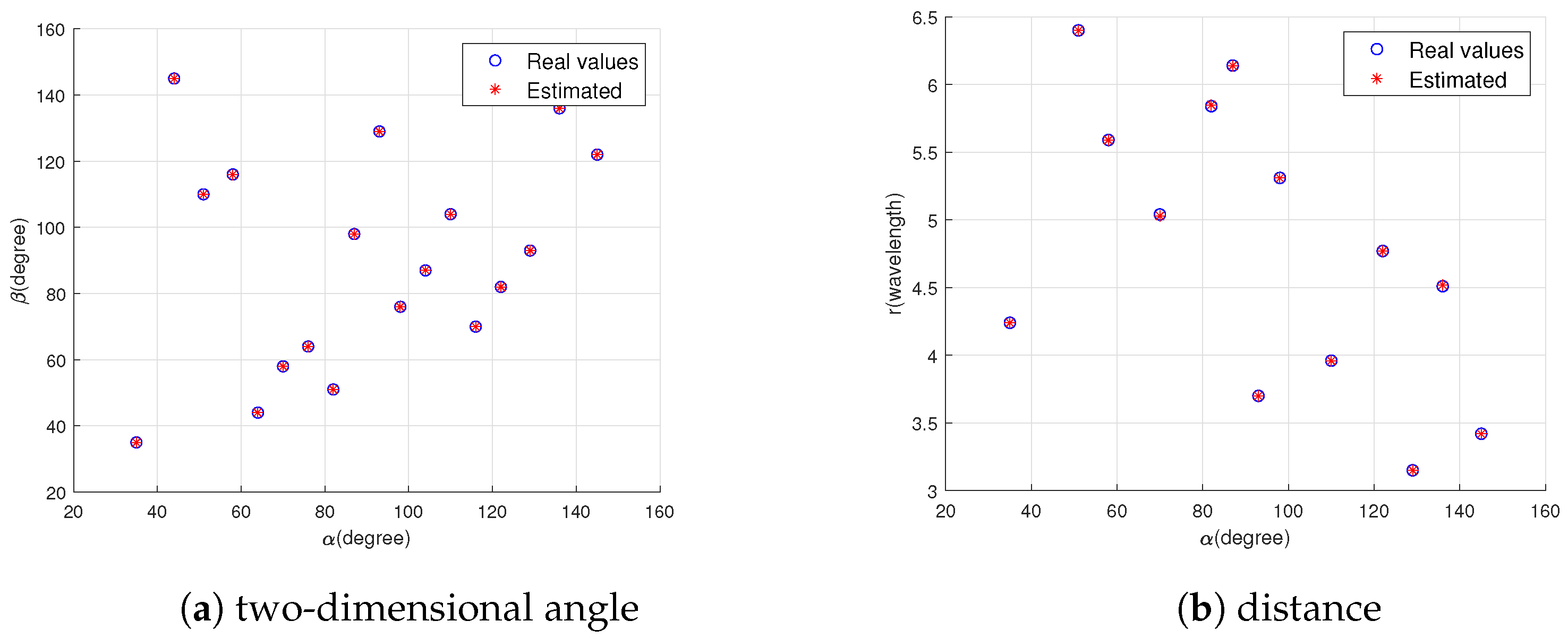
Experiment 1: Localization of Mixed NF and FF Sources. In this simulation, there are five narrowband FF sources and 13 narrowband NF sources in space. The number of elements on the positive half-axis of subarray 1 is set to $M_1=2$, for subarrays 2 and 3 to $M_2=M_3=2$, and for subarrays 4 and 5 to 1. The SNR is 30dB and the number of snapshots is 5200 (including 200 pseudo snapshots). The results are shown in Figure 2. It can be seen that, in scenarios where NF and FF sources coexist, the proposed algorithm can accurately estimate the 2D angle and range of the NF sources, as well as the 2D angle parameters of the FF sources, and correctly pair them, validating the superior performance of the proposed algorithm.

Experiment 2: RMSE versus SNR. There are two narrowband NF sources impinging from $\left\{{80}^{\circ },{70}^{\circ },5.12\lambda \right\}$ and $\left\{{130}^{\circ },{140}^{\circ },6.33\lambda \right\}$, respectively. Except for Challa’s algorithm, which sets 10 elements for each subarray on two axes with a total of 19 elements, the number of elements for each axis for all other algorithms is 9, resulting in a total of 17 elements. The total number of snapshots is set to 2200, including 200 pseudo snapshots. The SNR increases from 0 dB to 25 dB at a step size of 5 dB, and $\overline{M}$ is set to 500. The results are shown in Figure 3. It can be observed that the proposed algorithm has significantly better estimation performance for $\alpha$ and $\beta$ than the existing algorithms, as the SNR varies. For range estimation, the performance of the proposed algorithm is better than that of the other algorithms, too. Over the SNR interval 0–25 dB, the proposed algorithm remains close to the CRB, confirming its closer proximity to the theoretical limit compared with competing methods under the given array configuration and parameter set.

Experiment 3: RMSE versus snapshot. The RMSE result with respect to the number of snapshots is plotted in Figure 4, where the number of snapshots ranges from 400 to 4000, while other parameters are consistent with those in the third simulation. It is shown that the RMSE of DOA and distance estimation exhibits a monotonic improvement with SNR. The proposed algorithm outperforms subspace and optimization techniques based on uniform arrays when a small number of snapshots are available. The algorithm’s effectiveness stems from its ability to fully exploit the spatio-temporal information of received signals and the SENA framework, which generates significantly more virtual elements than the physical array. In addition, the comparison of algorithms’ runtime is shown in

Table 4. The runtime of different algorithms with snapshot = 3000.

Algorithm	Challa [38]	Liang [9]	Wu [37]	Proposed Algorithm
Runtime(s)	2.58	3.56	4.00	21.77

, where it can be seen that the proposed algorithm costs more runtime than others in exchange for performance improvement.

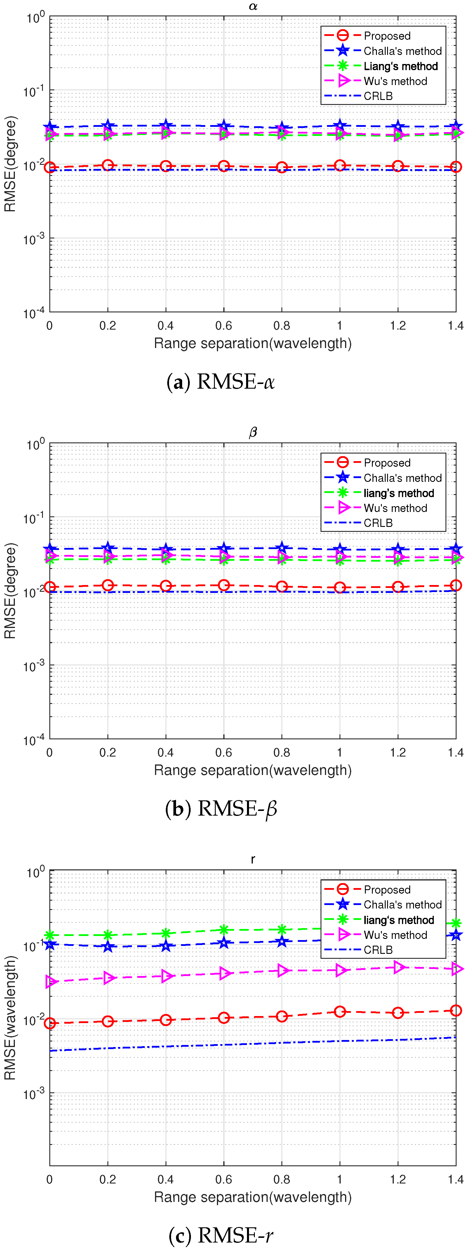
Experiment 4: RMSE versus range separation. The performance is examined by varying the range, while keeping the SNR and snapshot number fixed. The basic parameters are the same as in the third simulation. The SNR is set to 10, and the snapshot number is 2200, which includes 200 pseudo snapshots. The distance of the first signal is 3.2$\lambda$, and the distance of the second signal is 3.2$\lambda$ + $\Delta \lambda$, varying from 0.1$\lambda$ to 1.1$\lambda$. The results are presented in Figure 5, showing that while the angle estimation accuracy remains stable across varying distances, the distance estimation performance shows clear trend of degradation. The proposed algorithm still outperforms other methods as the range separation increases. It is demonstrated that, through effective utilization of spatial-temporal information with its SENA-based array structure that possesses a significantly larger number of virtual elements than the physical elements, the proposed algorithm still exhibits enhanced estimation performance.

6. Conclusions

A NF 3D parameter estimation algorithm based on a symmetric enhanced nested array is proposed, which jointly utilizes the spatial-temporal information of the received data and the FOC results. And the array aperture is analyzed, which obtains the maximum virtual aperture under different M1 and M2 conditions. Compared with other algorithms, the proposed algorithm has improved angle and distance accuracy by 65% and 61.7%, respectively. The viability of the proposed algorithm has been evidenced by the extensive simulation results provided.

References

1. Levy-Israel, M.; Bilik, I.; Tabrikian, J. MCRB on DOA Estimation for Automotive MIMO Radar in the Presence of Multipath. IEEE Trans. Aerosp. Electron. Syst. 2023, 59, 4831–4843. [Google Scholar] [CrossRef]
2. Sorkhabi, S.E.; Rambabu, K. Multi-Target DoA Estimation with mmWave MIMO Radar using Limited Number of Sensors. IEEE Trans. Veh. Technol. 2025, 1–13. [Google Scholar] [CrossRef]
3. Pote, R.R.; Rao, B.D. Maximum Likelihood-Based Gridless DoA Estimation Using Structured Covariance Matrix Recovery and SBL With Grid Refinement. IEEE Trans. Signal Process. 2023, 71, 802–815. [Google Scholar] [CrossRef]
4. Sakhnini, A.; Bourdoux, A.; Pollin, S. Estimation of Array Locations, Orientations, Timing Offsets and Target Locations in Bistatic Radars. IEEE Trans. Radar Syst. 2023, 1, 520–531. [Google Scholar] [CrossRef]
5. Chen, H.; Fang, J.; Wang, W.; Liu, W.; Tian, Y.; Wang, Q.; Wang, G. Near-Field Target Localization for EMVS-MIMO Radar With Arbitrary Configuration. IEEE Trans. Aerosp. Electron. Syst. 2024, 60, 5406–5417. [Google Scholar] [CrossRef]
6. Shamsian, M.R.; Sadeghi, M.; Behnia, F. Joint TDOA and DOA Single Site Localization in NLOS Environment Using Virtual Stations. IEEE Trans. Instrum. Meas. 2024, 73, 5500710. [Google Scholar] [CrossRef]
7. Yuan, S.; Fioranelli, F.; Yarovoy, A.G. Vehicular-Motion-Based DOA Estimation With a Limited Amount of Snapshots for Automotive MIMO Radar. IEEE Trans. Aerosp. Electron. Syst. 2023, 59, 7611–7625. [Google Scholar] [CrossRef]
8. He, J.; Swamy, M.N.S.; Ahmad, M.O. Efficient Application of MUSIC Algorithm Under the Coexistence of Far-Field and Near-Field Sources. IEEE Trans. Signal Process. 2012, 60, 2066–2070. [Google Scholar] [CrossRef]
9. Liang, J.; Liu, D. Passive Localization of Mixed Near-Field and Far-Field Sources Using Two-stage MUSIC Algorithm. IEEE Trans. Signal Process. 2010, 58, 108–120. [Google Scholar] [CrossRef]
10. Zhi, W.; Chia, M.Y.W. Near-Field Source Localization via Symmetric Subarrays. IEEE Signal Process. Lett. 2007, 14, 409–412. [Google Scholar] [CrossRef]
11. Xie, J.; Tao, H.; Rao, X.; Su, J. Efficient Method of Passive Localization for Near-Field Noncircular Sources. IEEE Antennas Wirel. Propag. Lett. 2015, 14, 1223–1226. [Google Scholar] [CrossRef]
12. Yan, H.; Chen, H.; Liu, W.; Yang, S.; Wang, G.; Yuen, C. RIS-Enabled Joint Near-Field 3D Localization and Synchronization in SISO Multipath Environments. IEEE Trans. Green Commun. Netw. 2025, 9, 367–379. [Google Scholar] [CrossRef]
13. Wu, X. Localization of far-field and near-field signals with mixed sparse approach: A generalized symmetric arrays perspective. Signal Process. 2020, 175, 107665. [Google Scholar] [CrossRef]
14. Guo, H.; Chen, H.; Liu, W.; Yang, S.; Yuen, C.; So, H.C. Third-Order Sum-Difference Expansion: An Array Extension Strategy Based on Third-Order Cumulants. IEEE Trans. Signal Process. 2025, 73, 2099–2109. [Google Scholar] [CrossRef]
15. Leite, W.S.; Lamare, R.C.d.; Zakharov, Y.; Liu, W.; Haardt, M. Direction Finding With Sparse Subarrays: Design, Algorithms, and Analysis. IEEE Trans. Aerosp. Electron. Syst. 2024, 60, 8149–8165. [Google Scholar] [CrossRef]
16. Chen, H.; Lin, H.; Liu, W.; Wang, Q.; Shen, Q.; Wang, G. Augmented Multi-Subarray Dilated Nested Array With Enhanced Degrees of Freedom and Reduced Mutual Coupling. IEEE Trans. Signal Process. 2024, 72, 1387–1399. [Google Scholar] [CrossRef]
17. Moffet, A. Minimum-redundancy linear arrays. IEEE Trans. Antennas Propag. 1968, 16, 172–175. [Google Scholar] [CrossRef]
18. Vaidyanathan, P.P.; Pal, P. Sparse Sensing With Co-Prime Samplers and Arrays. IEEE Trans. Signal Process. 2011, 59, 573–586. [Google Scholar] [CrossRef]
19. Pal, P.; Vaidyanathan, P.P. Nested Arrays: A Novel Approach to Array Processing With Enhanced Degrees of Freedom. IEEE Trans. Signal Process. 2010, 58, 4167–4181. [Google Scholar] [CrossRef]
20. Kulkarni, P.; Vaidyanathan, P.P. Weight-Constrained Sparse Arrays For Direction of Arrival Estimation Under High Mutual Coupling. IEEE Trans. Signal Process. 2024, 72, 4444–4462. [Google Scholar] [CrossRef]
21. Sarangi, P.; Hücümenoğlu, M.C.; Rajamäki, R.; Pal, P. Super-Resolution With Sparse Arrays: A Nonasymptotic Analysis of Spatiotemporal Trade-Offs. IEEE Trans. Signal Process. 2023, 71, 4288–4302. [Google Scholar] [CrossRef]
22. Chen, Y.P.; Liu, C.L. Half-Inverted Array Design Scheme for Large Hole-Free Fourth-Order Difference Co-Arrays. IEEE Trans. Signal Process. 2023, 71, 3296–3311. [Google Scholar] [CrossRef]
23. Patra, R.K. A Novel Third-Order Nested Array for DOA Estimation With Increased Degrees of Freedom. IEEE Signal Process. Lett. 2025, 32, 1475–1479. [Google Scholar] [CrossRef]
24. Shaikh, A.H.; Liu, X. Super Fragmented Coprime Arrays for DOA Estimation. IEEE Signal Process. Lett. 2025, 32, 1825–1829. [Google Scholar] [CrossRef]
25. S., J.; Yadav, S.K.; George, N.V. Coarray LMS: Adaptive Underdetermined DOA Estimation With Increased Degrees of Freedom. IEEE Signal Process. Lett. 2024, 31, 591–595. [Google Scholar] [CrossRef]
26. Sheng, X.; Lu, D.; Li, Y.; de Lamare, R.C. Enhanced MISC-Based Sparse Array With High uDOFs and Low Mutual Coupling. IEEE Trans. Circuits Syst. II Express Briefs 2024, 71, 972–976. [Google Scholar] [CrossRef]
27. Chen, H.; Guo, H.; Liu, W.; Shen, Q.; Wang, G.; So, H.C. Fourth-Order Sparse Array Design From a Sum-Difference Co-Array Perspective. IEEE Trans. Signal Process. 2025, 73, 2243–2254. [Google Scholar] [CrossRef]
28. Ebadi, Z.; Molaei, A.M.; Alexandropoulos, G.C.; Abbasi, M.A.B.; Cotton, S.; Tukmanov, A.; Yurduseven, O. Near-Field Localization With Antenna Arrays in the Presence of Direction-Dependent Mutual Coupling. IEEE Trans. Veh. Technol. 2025, 74, 7033–7048. [Google Scholar] [CrossRef]
29. Gast, A.; Le Magoarou, L.; Shlezinger, N. DCD-MUSIC: Deep-Learning-Aided Cascaded Differentiable MUSIC Algorithm for Near-Field Localization of Multiple Sources. In Proceedings of the ICASSP 2025—2025 IEEE International Conference on Acoustics, Speech and Signal Processing (ICASSP), Hyderabad, India, 6–11 April 2025; pp. 1–5. [Google Scholar] [CrossRef]
30. Fang, J.; Chen, H.; Liu, W.; Yang, S.; Yuen, C.; So, H.C. Three-Dimensional Localization of Mixed Near-Field and Far-Field Sources Based on a Unified Exact Propagation Model. IEEE Trans. Signal Process. 2025, 73, 245–258. [Google Scholar] [CrossRef]
31. Zheng, Z.; Fu, M.; Wang, W.Q.; Zhang, S.; Liao, Y. Localization of Mixed Near-Field and Far-Field Sources Using Symmetric Double-Nested Arrays. IEEE Trans. Antennas Propag. 2019, 67, 7059–7070. [Google Scholar] [CrossRef]
32. Wu, X.; Yan, J. A Second-Order Statistics-Based Mixed Sources Localization Method With Symmetric Sparse Arrays. IEEE Commun. Lett. 2020, 24, 1695–1699. [Google Scholar] [CrossRef]
33. Tian, Y.; Wang, X.; Jin, X.; Hou, Y. Near-field Source Location Estimation Algorithm Based on Coprime Array. In Proceedings of the 2022 IEEE International Conference on Signal Processing, Communications and Computing (ICSPCC), Xi’an, Chian, 25–27 October 2022; pp. 1–5. [Google Scholar] [CrossRef]
34. Su, X.; Hu, P.; Liu, Z.; Liu, T.; Peng, B.; Li, X. Mixed Near-Field and Far-Field Source Localization Based On Convolution Neural Networks via Symmetric Nested Array. IEEE Trans. Veh. Technol. 2021, 70, 7908–7920. [Google Scholar] [CrossRef]
35. Zheng, Z.; Fu, M.; Wang, W.Q.; So, H.C. Symmetric Displaced Coprime Array Configurations for Mixed Near- and Far-Field Source Localization. IEEE Trans. Antennas Propag. 2021, 69, 465–477. [Google Scholar] [CrossRef]
36. Wu, X.; Zhu, W.P. Single Far-Field or Near-Field Source Localization With Sparse or Uniform Cross Array. IEEE Trans. Veh. Technol. 2020, 69, 9135–9139. [Google Scholar] [CrossRef]
37. Wu, X.; Yan, J. 3-D Mixed Far-Field and Near-Field Sources Localization With Cross Array. IEEE Trans. Veh. Technol. 2020, 69, 6833–6837. [Google Scholar] [CrossRef]
38. Challa, R.N.; Shamsunder, S. Passive near-field localization of multiple non-Gaussian sources in 3-D using cumulants. Signal Process. 1998, 65, 39–53. [Google Scholar] [CrossRef]
39. Chen, H.; Yi, Z.; Jiang, Z.; Liu, W.; Tian, Y.; Wang, Q.; Wang, G. Spatial-temporal-based Underdetermined Near-field 3-D Localization Employing a Nonuniform Cross Array. IEEE J. Sel. Top. Signal Process. 2024, 18, 561–571. [Google Scholar] [CrossRef]
40. Yang, Z.; Xie, L.; Zhang, C. A Discretization-Free Sparse and Parametric Approach for Linear Array Signal Processing. IEEE Trans. Signal Process. 2014, 62, 4959–4973. [Google Scholar] [CrossRef]
41. Chen, H.; Wang, W.; Liu, W. Joint DOA, Range, and Polarization Estimation for Rectilinear Sources With a COLD Array. IEEE Wirel. Commun. Lett. 2019, 8, 1398–1401. [Google Scholar] [CrossRef]
Figure 1. 3D localization model for SENA of NF sources.
Technologies 13 00415 g001
Figure 2. Scattergram for mixed-source localization.
Technologies 13 00415 g002
Figure 3. RMSE versus SNR.
Technologies 13 00415 g003
Figure 4. RMSE versus the number of snapshots.
Technologies 13 00415 g004
Figure 5. RMSE versus range separation.
Technologies 13 00415 g005