1. Introduction
Industrial modernization has increased energy demand over the past decade. However, while supply is still limited, demand must rise faster than supply. The decreasing availability of resources such as, coal, petroleum, and natural gas has contributed to a growing imbalance between energy demand and supply, leading to an energy crisis. To mitigate pollution and alleviate pressure on conventional energy sources, researchers are exploring renewable energy resources such as wind, solar, geothermal, water, and biomass [
1,
2]. Solar radiation (SR) is a widely available renewable energy source in many regions around the world. In recent years, the focus on accurate and reliable SR prediction has intensified, driven by the need to optimize solar energy systems and enhance their efficiency. Accurate SR prediction improves the design and operation of solar power plants, leading to better energy management, reduced costs, and enhanced grid integration [
3,
4]. In this study, we focus on SR prediction, which plays a vital role in optimizing solar energy systems and improving the efficiency of renewable energy generation.
The literature has reported the prediction of SR using several ML models. Fan et al. compared SR prediction using Extreme Gradient Boosting (XGBoost) and SVM for SR prediction. They used the Turkish State Meteorological dataset. XGBoost performed the best regarding computational time and prediction accuracy [
5]. Edna et al. used the Brazilian National Institute of Meteorology dataset for SR prediction. They compare several ML algorithms, including Support Vector Regression (SVR), XGBoost, Categorical Boosting (CatBoost), and a Voting-Average (VOA) ensemble method. The authors reported that selecting ensemble features enhances forecasting performance, with the VOA method outperforming the other algorithms across various predictions [
6]. Wu et al. compared the Gradient Boosting (GB) and kernel-based nonlinear extension of Arps Decline (AD) models with categorical features to support daily global SR prediction using South China meteorological regional data. The AD model provided the best prediction accuracy, while the GB model provided the smallest computational time reported for SR [
7]. Basaran et al. developed bagging and boosting ensemble models of SVM, decision tree (DT), and ANN models for SR prediction using five years of meteorological and air pollution data from Beijing, China. The results demonstrated that ensemble models achieved higher performance than individual base models [
8].
Ibrahim and Khatib developed a firefly algorithm to select the optimal number of leaves per tree in the RF for the hourly global SR, utilizing meteorological data from Malaysia. The results indicated that the RF-FFA-optimized model surpassed the conventional RF, ANN, and ANN-FFA models in terms of accuracy and computational time [
9]. Gupta et al. developed an SR prediction system using Particle Swarm Optimization (PSO) to optimize RF parameters. The results showed that the optimized RF improved the individual DT, RF, and ANN for the prediction of SR [
10]. Srivastava et al. compared RF, classification and regression tree (CART), multivariate adaptive regression splines (MARS), and M5 tree-based ML models for SR prediction. RF outperformed the other models [
11]. Benali et al. compared intelligent persistence, RF, and ANN to predict SR using components of solar irradiation, which are diffuse horizontal, beam normal, and horizontal components in France. They reported that RF predicted all components more effectively than other methods [
12]. Belmahdi et al. compared seven ML models for SR prediction and reported that RF models had a more reliable SR forecast prediction [
13]. Guermoui et al. reported that they developed a hybrid ML model that utilizes a convolutional neural network, an extreme learning machine, a least squares SVM, and a nonparametric Gaussian process regression for multihour global SR prediction. The experimental results showed that the hybrid deep learning (DL) model approach achieved better accuracy than other popular ML models [
14]. Faisal et al. used a Recurrent Neural Network, Gated Recurrent Unit (GRU), and Long Short-Term Memory for a predicted SR [
15]. The GRU outperformed all other models. Geshnigani et al. used conventional Multiple Linear Regression, an Adaptive Neuro-Fuzzy Inference System, and a Multilayer Perceptron Neural Network using several optimization algorithms [
16]. The ANFIS with the genetic algorithm model effectively enhanced the prediction of the SR. Wu et al. used the Cuckoo Search, Gray Wolf Optimization (GWO), and Ant Colony Optimization algorithms to improve the SVM model capabilities for SR prediction. The findings showed that GWO-SVM gained the best results [
17]. These studies indicate that optimization-based feature selection can improve model performance compared to using all available features.
Goliatt and Yaseen used a computationally intelligent model that hybridized Covariance Matrix Adaptive Evolution Strategies (CMAES) with XGBoost and MARS models. CMAES managed the internal parameters of the XGBoost and MARS models and produced a hybrid approach for daily SR prediction. The results demonstrated that the hybrid approach enhanced prediction accuracy [
18]. The variance inflation factor and mutual information were used by Gupta et al. to choose the most important features to feed into a stack ensemble extra trees model for SR prediction. Results showed that the ensemble model with selected features effectively reduced prediction errors [
19].
The literature highlighted that ML and DL models are highly effective tools for SR estimation. Researchers have used diverse datasets from various geographical locations, including India, France, Brazil, China, and Bangladesh, to enhance SR prediction accuracy. However, several challenges arise from the inherent variability of SR across different regions and seasons. Numerous factors influence SR prediction, varying widely across geographical locations and seasons. Training a model on data from one geographical region may not translate well to another, resulting in inaccuracies. The literature also indicates that applying feature selection techniques based on optimization and hybrid models can enhance the performance of individual models.
Despite their success, many of these models operate as opaque systems, hindering the interpretation of results and decision-making processes. This complexity can hinder trust and acceptance in critical energy applications that require reliable decision-making. XAI techniques help make these models more transparent and interpretable. Song et al. applied the SHAP-based XAI method to tree-based ensemble models, facilitating a clear understanding of feature importance and interaction effects in SR prediction [
20]. In the same way, Nallakaruppan et al. employed LIME to elucidate the impact of critical parameters such as solar irradiance and temperature on energy yield, thereby improving model transparency [
21]. In this study, we compare the performance of a set of ML models for SR prediction using a publicly available dataset collected from different site locations in Saudi Arabia, facilitating broader model generalization. The best-performing model is further analyzed using two XAI techniques, LIME and SHAP, to provide global and local explanations. Building on this, we employ LIME and SHAP not only for global and local explanations of the best-performing model but, distinctively, to guide feature selection for retraining and optimizing this model’s explanations. Unlike previous works, we leverage XAI methods not only to better understand the feature space but also to identify the most impactful features for SR prediction, which are subsequently used to retrain the best model. This approach enhances the SR prediction system’s performance, interpretability, and trustworthiness. The paper offers the following key contributions:
Improve SR prediction by using the XAI-based feature selection method for SR prediction.
Evaluate and compare six ML models using a publicly available dataset and a set of quantitative measures.
Analyze the top-performing model among the evaluated techniques using SHAP and LIME XAI methods to quantify feature contributions and select the most influential features.
Use selected features as inputs to the best model to optimize its efficiency and performance.
The organization of this paper is as follows: A detailed analysis of the SR dataset, ML models, and XAI techniques is provided in
Section 2.
Section 3 presents the statistical metrics to evaluate the ML models;
Section 4 compares the models and discusses XAI-selected features. Finally, concludes the paper.
2. Materials and Methods
SR provides a clean and sustainable solution, helping to reduce greenhouse gas emissions and combat climate change. The quantity of SR obtained depends on several factors, including geographic location and meteorological conditions. As shown in
Figure 1, the system outlines the workflow for feature selection influenced by XAI methods in conjunction with ML models and the evaluation parameters used for performance assessment. This approach promotes the identification of the most relevant features for model prediction while enhancing transparency and interpretability in SR prediction.
The Atomic and Renewable Energy Department at King Abdullah City in Saudi Arabia collects and maintains a publicly available SR prediction dataset. The dataset is available on the OpenData platform, a Saudi Arabian government repository for all experimental evaluations. It consists of 1265 records, each defined by 26 unique features. These features represent different parameters related to solar power generation and meteorological conditions. The data was gathered from 41 solar power plants across Saudi Arabia between 2017 and 2021.
Table 1 provides an organized list of solar power facilities and corresponding records in the dataset. The minimum number of records was obtained from Princess Norah University, with six records, while the maximum was collected from K.A. CARE Olaya and K.A. CARE City, with 42 records each. This dataset reflects the variability of SR across diverse locations in Saudi Arabia. It is crucial for developing accurate predictive models. The mean and standard deviation of GHI are 30.853 and 8.777 across all records before normalization. These statistics are essential for understanding the dataset’s distribution and enhancing the reliability of the predictive models.
We performed several preprocessing steps to enhance the predictive efficacy of the dataset. The preliminary analysis of the data revealed the absence of the attribute “Wind Speed at 3 m (SD) Uncertainty (m/s)” for all site locations, leading to its exclusion from the dataset. The dataset excludes four records that lack sun radiation values.
Table 2 summarizes the count of missing values for each feature in the dataset. Wind-related variables (e.g., wind speed, wind direction, peak wind speed, and their uncertainties) each have around 60–62 missing values, accounting for approximately 4.7% to 4.9% of the data. Both DHI and DNI have minimal missing values. Standard deviation components (e.g., for DHI, DNI, and GHI) exhibit significantly higher missingness, with around 260–264 missing entries, or roughly 20.6% of the dataset. Additionally, non-predictive metadata fields (e.g., date, latitude, and longitude) were excluded after feature engineering. The mean values of the respective features were used to substitute the missing values in all other imputed data. Subsequent to processing, each feature was subjected to independent normalization, resulting in a mean of zero and a standard deviation of one. All features were normalized using StandardScaler scaling. Similarly, we set the SR values, which are shown by the Global Horizontal Irradiance (GHI) scale, using the Min-Max Scaler to account for differences in how much power different solar stations produce.
Table 3 presents detailed statistics for all the features in the dataset. The final dataset consists of 1261 records and 21 attributes.
2.1. ML Models
ML models offer diverse approaches to regression tasks, each with unique strengths and motivations. When evaluating ML model performance, factors such as interpretability, model complexity, computational efficiency, and the nature of the data, such as linear and non-linear, play a crucial role in determining the most proper model.
Linear Regression (LR) establishes a linear relationship between input features and the output variable, and it is one of the simplest ML models. Its strength lies in its ease of implementation and interpretability, particularly when the data displays linear trends. SVR extends the principles of SVM to regression, employing kernel functions to handle non-linear patterns effectively, making it a versatile option for diverse datasets. RF offers further improvements by combining multiple decision trees to create a robust, stable model. RF is known for reducing overfitting and handling noisy data, making it well-suited for complex, non-linear datasets with large feature spaces. BR integrates prior beliefs into the regression model by treating model parameters as probability distributions; it is functional when uncertainty quantification is crucial. The GBR builds models sequentially by minimizing errors from previous models, resulting in a robust prediction model that boosts weak learners. An ANN functions similarly to a human neuron system, consisting of interconnected layers of neurons capable of capturing complex patterns in data. The ANN features multiple fully connected hidden layers between the input and output layers with ReLU activation. It is connected to every neuron in the preceding and following layers, enabling the network to capture intricate data patterns [
22]. An output layer with a linear activation function suitable for regression tasks. Its ability to model non-linear interactions makes it powerful for large datasets where traditional models may struggle to capture underlying data dynamics.
2.2. Explainable AI
XAI refers to techniques designed to enhance transparency and interpretability by making the decisions and predictions of AI models understandable to humans. As ML models become more complex, their “black box” nature poses challenges for users attempting to comprehend their decisions. XAI techniques offer insights into the influence of input features on model predictions, either locally or globally. This work explores two techniques: Local Interpretable Model-agnostic Explanations (LIME) and Shapley Additive Explanations (SHAP). LIME focuses on local interpretations, while SHAP provides a global perspective, making the two techniques complementary within the field of XAI [
23].
2.2.1. LIME
Ribeiro et al. introduced LIME to bridge the gap between human and AI systems by providing precise and local explanations of model predictions [
24]. LIME operates independently of the internal workings of the ML model and focuses on explaining predictions at the data level.
For input feature x, LIME identifies the interpretable model by minimizing the loss and the complexity regularization as , where represents the complexity of the explanation model and the minimizing promotes the selection of simpler and more interpretable models, while a small ensures that the chosen model accurately reflects the predictions of the underlying model. The proximity function captures how similar perturbed instances are to the instance being explained. LIME provides a reliable local explanation for a model with complex global interpretation, where “locality” is defined by . LIME perturbs the input features based on the statistical characteristics of the training data to generate explanations for specific predictions.
2.2.2. SHAP
This technique is rooted in cooperative game theory that allocates significance to each feature based on its contribution to the model’s decision-making process [
25]. The value for a feature
i is calculated as
where
N is the total number of features and
is a set of all possible combinations of features.
S is a subset of features in
N,
is the model’s prediction when using only the features in subset S, and
is the SHAP value indicating the contribution of feature i to the prediction.
is the cumulative contribution value of feature
j. The Shapley value ensures that each feature’s contribution is fairly evaluated by considering all possible combinations of features. In addition to computing individual feature contributions, the SHAP maintains the property of additivity, which can be expressed in the equation
Here,
represents the model’s prediction for input
x, and
is the average prediction across the dataset. This equation confirms that the total contribution to model prediction is averaged over all different combinations of features. The Shapley value has various valuable properties such as additivity, symmetry, dummy, and efficiency [
26,
27]. The additivity property requires that the aggregate sum of individual models’ predictions matches the combined model’s prediction. Symmetry means features with equal contributions to the model receive the same Shapley values. The dummy property states that if a feature’s marginal contribution is zero across all possible models, its Shapley value will also be zero. The efficiency means that the sum of all feature contributions equals the difference between the model’s prediction and the average [
27]. The SHAP values are consistent and interpretable to obtain global insights into feature importance and influence on complex ML model predictions.
3. Experiments and Results
SR prediction models were implemented using the Python-based Scikit-Learn library. All the experiments were conducted on a Windows 10 operating system with an Intel i7 3.13 GHz processor and 64 GB of RAM. The optimum hyperparameter for these models based on cross-validation is listed in
Table 4.
3.1. Evaluation Metrics
The ML models are assessed using five measurements: MAE, RMSE, RMSRE,
, PC, and MAPE. The metrics are selected based on SR prediction literature and are defined as follows:
where
N is the number of SR values recorded,
is the ith measured SR value,
is the
ith predicted SR value, and
is the mean of the measured SR values.
MAE and MSE range from 0 to ∞, and both are better when lower, indicating smaller prediction errors. R2 ranges from to 1, with higher values closer to 1 being better, signifying a better model fit. The PC quantifies a linear relationship between two variables, ranging from −1 to +1, where negative and positive values represent a perfect negative and positive correlation, respectively. A zero PC signifies no linear correlation. This helps analysts understand how closely related the predictor and response variables are. MAPE measures the average percentage difference between the and . The RMSER calculates the square root of the mean of squared relative errors, normalized by the . It provides a scale-independent measure of error.
3.2. Predictive Performance
In
Table 5, each station was iteratively used as the test set, while the remaining stations served as the training data, a strategy known as leave-one-station-out cross-validation.
Table 5 represents the performance averaged across all such station-wise evaluations.
The observed results indicated that the RF model performed the best in terms of accuracy and generalizability across different sites. The MLP reported overfitting or poor generalization, indicating a need for tuning, more data, or regularization. The RF and GBR demonstrate excellent generalization, making them suitable for real-world deployment.
A comparative analysis of six ML models using three measures is presented in
Table 6. Each model is trained using a complete feature set and is 10-fold cross-validated, and the mean and standard deviation (SD) of each measure across all folds are used for comparison. The LR, the simplest ML model, performs the worst in all measures due to its limited linear nature. The SR prediction using SVM improved significantly compared to LR. The GB performs well but is slightly less accurate than RF, BR, and ANN. RF and BR perform similarly, outperforming LR, SVR, and GB. The ANN model performs best among all ML models. ANN achieved the best performance with the lowest MAE of 0.0093, RMSE of 0.0127, and the highest
of 0.9913. The MAPE and RMSRE values are also the lowest compared to other models. It is observed that percentage-based metrics such as MAPE and RMSRE exhibit high standard deviations relative to their mean values (e.g., MAPE: 1.4728 ± 2.3999). This high variability is attributed to the sensitivity of these metrics to small true target values in the solar radiation dataset. When true values approach zero, even small absolute errors can result in disproportionately large percentage errors, leading to outliers and skewed distributions. The ANN model’s ability to capture complex, non-linear patterns and interactions between features makes it the most accurate and reliable choice for SR prediction. The Adam optimizer (Adaptive Moment Estimation) gives computational efficiency and a minimal memory requirement, making it well-suited for ANN models with large datasets and complex architectures [
28]. The learning rate was set to 0.01 to ensure stable and efficient convergence of the ANN model.
Table 7 presents the architecture of the proposed ANN model and the configuration details of its layers, output shapes, and parameters. The model contains three dense layers with 64, 32, and 1 neurons, respectively. The model uses 3521 parameters, demonstrating its complexity and learning capacity. The model provides a detailed equation for calculating the parameters [
29]. The ANN model is fitted with a training set of a batch size of 32 and runs for 200 epochs. With this configuration, we can train the model iteratively, updating the weights after each batch of 32 samples. We compile the models using the MSE as the loss function, a standard regression task metric. We design the ANN architecture to balance complexity and performance, enabling the model to effectively learn from the training data while maintaining its generalization capabilities.
Figure 2 compares the performance of different ML models using various evaluation metrics. When comparing models across the metrics such as MAE, RMSE, and MAPE, a lower median and a smaller spread within the box plot indicate better and more stable performance. A low median suggests that the model consistently achieves minimal errors. This figure highlights the importance of evaluating central tendencies and data distribution to ensure robust and reliable model performance. The ANN model archives the minimum values of MAE, RMSE, and MAPE. The ANN model exhibits the highest
score among all the ML models, signifying its strong ability to explain the variance in the dataset. Hence, the trained ANN model is investigated using XAI techniques.
3.3. XAI-Based ANN Optimization
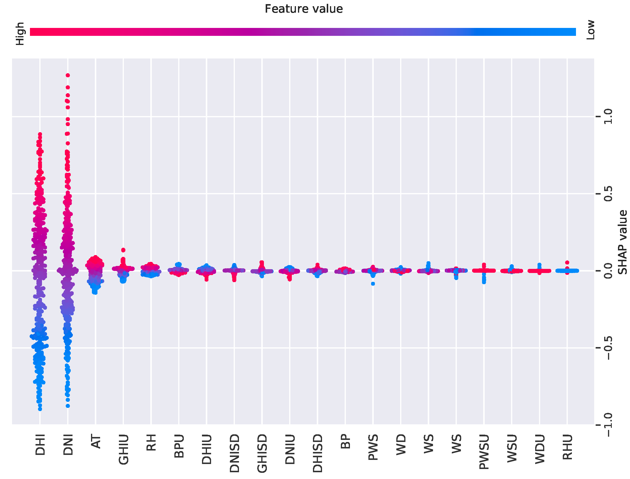
SHAP and LIME are effective tools for interpreting ML models, transforming black-box models into white-box models and enabling better local and global analysis. See
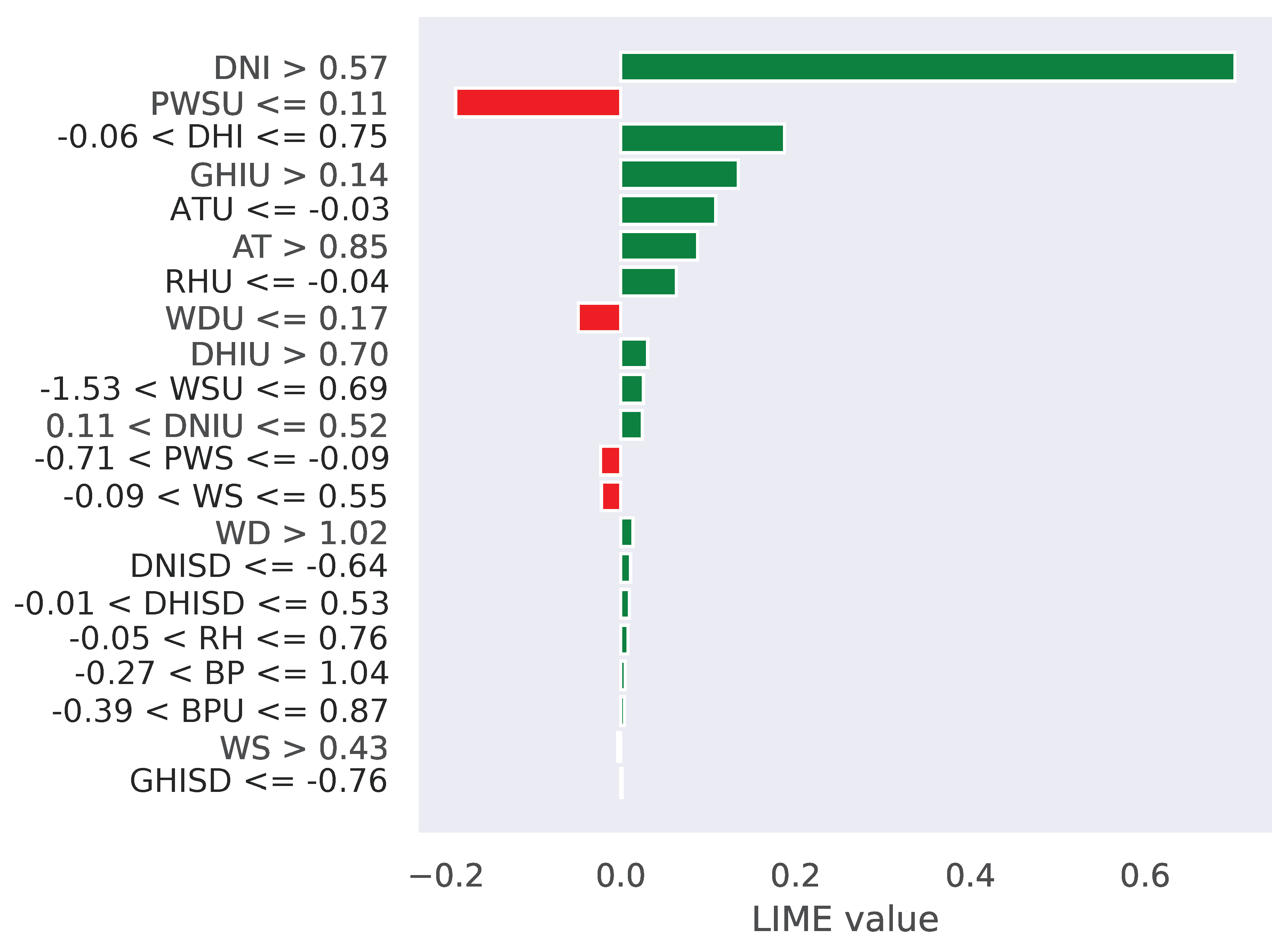
Figure 3. For global interpretation, the output using SHAP for the ANN model revealed that the first features in red are the most contributory ones for SR prediction. Additionally, the local interpretation by the LIME, shown in
Figure 4, indicated that the green features (DNI, DHI, GHIU, ATU, and AT) had a positive effect on the output. These figures demonstrate how SHAP and LIME techniques provided a clearer understanding of the most informative features influencing SR prediction. In this case, selecting only the most informative features simplifies the model structure and could improve generalization and accuracy and reduce both training times and the risk of overfitting [
30,
31]. XAI eliminates features that add little value to reduce the complexity of the ANN. This results in faster training times and less risk of overfitting, where the model learns noise instead of meaningful patterns. In this case, selecting only the top five features simplifies the model structure and may improve generalization and accuracy.
The ANN model is retrained using features selected through XAI-based methods. This improved version of the model is called the optimized ANN. The details of the optimized ANN parameters are shown in
Table 8. The optimized ANN model achieved an MAE of 0.0024, RMSE of 0.0111,
of 0.9980, and PC of 0.9966, comparatively more increased than the base model. This approach shows that using XAI to select key features can lead to better results while minimizing model complexity. The relative change (RC) in terms of a performance metric is calculated as
Table 9 presents the comparative performance of the best ANN model using all features and the optimized ANN model using the top five features. The optimized model performs better, with a decrease in MAE and RMSE and an increase in
and PC. The optimized ANN model requires less computation and memory, making it more efficient. The optimized ANN’s average inference time is 0.000358 s with
Floating Point Operations (FLOPs) in K. Similarly, for ANN, it is 0.000506 s with
. XAI contributes to this by streamlining the input data, which reduces the ANN’s overall training time and inference cost. This is particularly important in practical applications requiring large-scale data and real-time predictions.
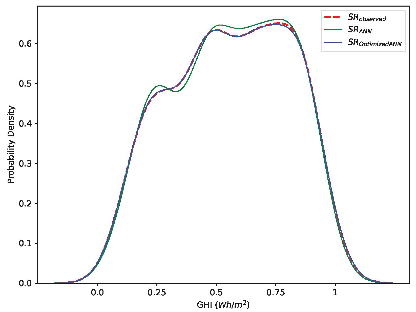
The comparison of Kernel Density Estimation (KDE)-based probability density for SR observed data, standard ANN, and optimized ANN is shown in
Figure 5. The figure indicates the effectiveness of model optimization in replicating the observed SR data’s distribution. The initial ANN model’s KDE shows some discrepancies due to its inability to make perfect predictions. The optimized ANN’s KDE closely matches the SR observed data, indicating that the optimization process successfully tunes the model to predict the data’s characteristics better. This similarity between the observed and optimized ANN KDEs signifies that the model has improved in capturing central tendencies, variability, and other statistical properties, offering more accurate and reliable predictions.
DHI, DNI, AT, GHIU, and RH are the most important features selected through XAI techniques for SR prediction. DHI represents the amount of solar radiation received per unit area by a horizontal surface that comes indirectly from the sky. Similarly, DNI quantifies the SR received in a direct beam on a surface perpendicular to the sun’s rays. AT is particularly influential in SR measurements, as it can affect the atmospheric conditions that scatter SR, impacting both GHI and DNI values. The uncertainty is the error, or variability, in the recorded values. These uncertainties can arise from various factors, including instrument calibration, atmospheric variability, and data processing methodologies. The RHU indicates the uncertainty or measurement error/margin associated with the relative humidity. According to the XAI analysis, these features are important for accurate SR prediction. Understanding their relationships and influences enhances the robustness of predictive models, ultimately improving the efficiency and reliability of solar energy systems. These features were selected based on their global importance ranking from the SHAP analysis. XAI contributes to this by streamlining the feature selection process, which has the potential to reduce the complexity and training time. A detailed ablation study to empirically validate this effect is planned as part of future work.


