Time-to-Fault Prediction Framework for Automated Manufacturing in Humanoid Robotics Using Deep Learning

Abstract

Industry 4.0 is transforming predictive failure management by utilizing deep learning to enhance maintenance strategies and automate production processes. Traditional methods often fail to predict failures in time. This research addresses this issue by developing a time-to-fault prediction framework that utilizes an enhanced long short-term memory (LSTM) model to predict machine faults. The proposed method integrates real-time sensor data, including current, voltage, and temperature calibrated via ultra-sensitive optical sensing technologies based on the typical whispering gallery optical mode (WGM) to create a robust dataset. Due to the high-quality factor that these sensors exhibit, any minute change on the surrounding medium will makes a significant change on its transmission spectrum. The LSTM model trained on these data demonstrated rapid and stable convergence, outperforming other deep learning techniques with a mean absolute error (MAE) of 0.83, a root mean squared error (RMSE) of 1.62, and a coefficient of determination (R²) of 0.99. The results show the superior performance of LSTM in predicting machine failures early in real-world environments within 10 min lead time, improving productivity and reducing downtime. This framework advances smart industries by improving fault prediction in manufacturing precision robotics components, demonstrated through two humanoid robots, GUCnoid 1.0 and ARAtronica.

1. Introduction

Industry 4.0 is transforming manufacturing through the integration of automation, data exchange, and artificial intelligence, improving efficiency and product quality across various sectors. These advancements are reshaping traditional manufacturing systems and optimizing operations. Effective control, monitoring, and maintenance of production equipment are crucial to ensuring high-quality and efficient manufacturing processes [1,2,3,4]. Sensors are pivotal to the effective operation of a wide range of industrial machinery, including systems such as packaging lines, hydraulic presses, turbine engines, heat exchangers, and computer numerical control (CNC) milling machines. Ensuring these components remain in optimal working condition is crucial, as any malfunction can disrupt the entire production process. To prevent such disruptions, continuous monitoring is employed, along with two primary maintenance strategies such as corrective maintenance and scheduled maintenance. Corrective maintenance is reactive, addressing critical equipment failures when they occur, which often results in unplanned production line downtimes. Scheduled maintenance is proactive, involving regular inspections and replacements to avert unexpected failures [2,5,6].

While scheduled maintenance is less disruptive, both strategies can still cause production losses and added costs. To reduce these issues, industries are adopting condition-based maintenance, which uses predictive assessments to schedule maintenance. This approach is integral to smart industrial maintenance practices, reducing the frequency of unplanned downtimes and avoiding unnecessary maintenance, thereby lowering costs and improving overall efficiency [2,4,6,7,8,9,10]. By integrating smart sensor systems and data analytics, industries can proactively monitor equipment health, detect early signs of failure, and optimize maintenance schedules to prevent unplanned downtimes. These sensors facilitate the connection of devices and systems, enabling machine communication for the continuous monitoring of industrial systems. By processing data locally and enabling rapid decision-making, sensors enhance product quality, reduce production costs, and boost operational efficiency. The evolution of sensor technologies, combined with innovations like big data, artificial intelligence, and cloud computing, is pushing industry 4.0 towards smarter, more automated production environments. This shift is creating new commercial opportunities as sensors become increasingly integral to driving innovation and maintaining market competitiveness [11].

In the manufacturing sector, both machines and operators encounter daily challenges related to managing vast amounts of data and customizing production processes. Predictive maintenance has emerged as a crucial strategy for anticipating equipment failures through advanced analytics, optimizing process efficiency, and enabling proactive resource management. This approach is essential in achieving operational excellence in manufacturing operations [12,13,14,15,16]. Given the growing volume of data generated in industries, the use of advanced techniques to develop accurate prediction models has become essential. Machine learning techniques have proven particularly effective in this context, utilizing algorithms to analyze data in real-time and predict outcomes [17]. These techniques enable comprehensive analysis and empower strategic decision-making based on large datasets, addressing the challenges of data variety, velocity, and volume in industrial settings [12].

Numerous studies have highlighted the value of artificial intelligence techniques in providing actionable insights for decision-making related to machine failures in industrial environments. Machine learning methods, such as artificial neural networks (ANNs), regression trees (RTs), random forests (RFs), and support vector machines (SVMs), are increasingly employed for regression and prediction tasks across different applications [9,18,19,20,21,22,23,24,25,26,27]. These techniques have paved the way for the development of predictive condition monitoring systems and remaining useful life (RUL) systems, which leverage a diverse range of production variables to anticipate equipment and machine failures and optimize maintenance strategies [9,28,29,30].

Beyond traditional industrial settings, predictive maintenance is vital in the production of precision components for advanced robotics, particularly humanoid robots. For instance, GUCnoid 1.0, humanoid robot equipped with a flexible spine [31], and ARAtronica, a telepresence humanoid robot equipped with two human-like arms and a Telepresence Camera for remote interaction, both require Teflon parts to achieve smoother and more durable rotational motion for their mechanical structures. These parts demand an exceptional level of precision that cannot be achieved through standard 3D printing methods. Automated industrial turning machines play a key role in fabricating such components, and implementing a fault prediction framework ensures consistent production quality while minimizing machine downtime during the manufacturing of these vital humanoid robot parts.

This research advances predictive fault detection by introducing a novel framework that integrates ultra-sensitive whispering gallery mode (WGM) optical sensors for precise data calibration of current, voltage, and temperature. Unlike traditional approaches, the proposed system utilizes real-time sensor data from a customized industrial turning machine. To overcome the limitations of scarce real-world failure data, an innovative method is employed to artificially generate time-to-failure datasets, enabling controlled training of the enhanced long short-term memory (LSTM) model. The enhanced LSTM model converges rapidly and stably, outperforming other models with a mean absolute error (MAE) of 0.83, a root mean squared error (RMSE) of 1.62, and a coefficient of determination (R²) of 0.99. This approach is specifically applied to the manufacturing of high-precision components for humanoid robotics, a unique focus in predictive maintenance research, and aims to achieve accurate fault predictions within a critical 10 min lead time, improving productivity, saving costs, and reducing downtime.

The framework is specifically developed for predicting faults in turning machines that are used in the manufacturing of high-precision components required for humanoid robots. These robots rely on intricate mechanical structures and therefore require components with a high degree of precision and durability. Predictive maintenance is thus paramount to minimize downtime in the manufacturing process of these critical parts. While the proposed methodology is applicable to other industrial applications, this work focuses on the field of advanced robotics. The key contributions of this paper are outlined as follows:

• Developing a novel time-to-fault prediction framework using an enhanced LSTM model to predict machine failures in industrial turning machines, offering 10 min of lead time to reduce downtime and enhance productivity.
• Creating a novel dataset by integrating real-time sensor data, including current, voltage, and temperature, from a customized turning machine provides a robust foundation for fault prediction.
• Exploiting the use of ultra-sensitive WGM-based optical sensors for calibration with high-precision data acquisition (current, voltage, temperature) technologies.
• Comparing three time-to-fault prediction scenarios in a real environment by analyzing actual failure time and the model’s performance, offering insights into its robustness and accuracy under varying operational conditions.
• Using the enhanced LSTM model, which demonstrates rapid and stable convergence, outperforming other deep learning techniques with an MAE of 0.83, an RMSE of 1.62, and an R² of 0.99.

This paper is structured into sections: Section 2 presents literature reviews; Section 3 describes the methodologies applied in system development; Section 4 shows the results of predictive tests and accuracy assessments; Section 5 presents challenges and limitations; and Section 6 discusses conclusions and future work.

2. Related Works

Industry 4.0 is revolutionizing industries by integrating advanced technologies such as the internet of things (IoT) and machine learning, driving predictive maintenance in accurate fault prediction, and efficient management of industrial assets. In industrial asset management, condition-based maintenance is a pivotal strategy focused on reducing unnecessary maintenance tasks, minimizing downtime, and lowering associated costs. This strategy revolves around three essential components, which are fault diagnosis, fault prognosis, and the optimization of maintenance procedures [7,8,10]. Fault diagnosis systems (FDSs) play a critical role in identifying and detecting faults, especially when system parameters or behaviors deviate from established norms [32,33,34]. Extensive research has been conducted on FDSs, addressing both small, localized systems and larger, more complex systems [32,33,34]. These systems are typically classified into two primary methodologies, like model-based approaches and model-free techniques. The model-based approach utilizes mathematical models to simulate the expected behavior of the monitored system, facilitating anomaly detection through comparison with actual performance. In contrast, model-free techniques apply machine learning algorithms to analyze historical data, identifying and classifying faults based on patterns and anomalies [33,34,35]. For instance, Ntalampiras developed a model-free FDS specifically for smart grids (SGs), utilizing physical layer data to effectively detect and isolate faults within the grid’s infrastructure [33]. While FDSs are primarily focused on detecting and classifying faults, fault prediction systems aim to forecast future equipment behavior and assess the likelihood of potential failures, which is crucial for making informed maintenance decisions.

Yildirim, Sun, and Gebraeel developed an advanced predictive framework aimed at refining maintenance strategies. Their approach utilizes Bayesian prognostic methods to dynamically estimate the remaining useful life of electric generators, thereby optimizing maintenance scheduling and cost forecasting [7,8]. This framework not only enables accurate predictions of maintenance costs, but also optimizes the scheduling of maintenance activities. Similarly, Verbert, Schutter, and Babuška developed a methodology for optimizing maintenance through effective failure prediction, utilizing a multivariate, multiple-model framework based on Wiener processes to model and predict equipment degradation [10]. This approach underscores the interconnection between fault diagnosis, fault prognosis, and maintenance process optimization, with ANNs being particularly noteworthy for their ability to perform predictive tasks with high accuracy and efficiency.

The rapid advancement of high-performance technologies has led to a significant surge in data collection, driven largely by the extensive integration of IoT devices. Sensors, crucial for capturing environmental data, have become indispensable across a broad spectrum of industries, including manufacturing, transportation, energy, retail, smart cities, healthcare, supply chain management, and agriculture [11,36,37]. The strategic implementation of IoT devices and sensors offers substantial opportunities for companies, yet it demands careful analysis to ensure successful deployment and a positive return on investment [11,36,37].

Recent research has increasingly highlighted the importance of advanced techniques such as machine learning and neural networks in predicting and diagnosing industrial failures. For instance, extreme learning machine (ELM) is introduced for diagnosing bearing failures, while other studies have developed models to assess the condition of rotating components [38,39,40]. The study employed an SVM-based system, whereas the authors combined SVM with feature selection methods like ReliefF and PCA, demonstrating the effectiveness of machine learning and feature selection in this domain [37,38,39,40,41,42,43,44,45,46,47,48,49,50,51,52,53]. Furthermore, a hybrid method for fault classification in power transmission networks is proposed, integrating feature selection via neighborhood component analysis (NCA) to enhance the precision of diagnostic strategies [52]. Moreover, some research has developed a model for predicting failures in beam–column junctions, employing various machine learning techniques, including KNN, linear regression (LR), SVM, ANN, DT, RF, ET, adaboost (AB), light gradient boosting machines (GBDTs), and extreme gradient boost (XGBoost), showcasing the versatility of machine learning approaches [54]. Research has increasingly delved into predicting failures in high-pressure fuel systems and forced blowers [38,39,40,41,42,43,44,45,46,47,48,49,50,51,52,53,54,55]. These investigations have utilized an array of advanced methodologies, including LR, RF, extreme gradient boosting (XGBoost), SVM, and artificial neural network multilayer perceptron (MLP). A significant body of research is dedicated to the development of machine learning algorithms, signal processing methods for sensor-acquired data, and image processing techniques for detecting visual anomalies in mechanical components [38,39,51,52,53,54,55,56,57,58,59]. These studies contribute to improving the efficiency, reliability, and safety of industrial operations, thus supporting predictive maintenance and reducing unplanned downtimes.

Some studies specifically tackle industrial challenges by identifying the most relevant variables and machine learning algorithms for predicting machine failures, which can adversely affect production planning. The insights from these studies are invaluable for guiding industries in selecting the most effective sensors and data collection methods for predicting machine failures [60]. A major advantage of ANNs is their high generalizability, allowing them to process data beyond the training set [21,30,61]. Li, Ren, and Lee demonstrated how ANNs could be used to predict wind speed, mitigating the effects of wind instability and enhancing energy generation efficiency by processing wind velocity data into average speed and turbulence intensity [62]. In railway engineering, research efforts have focused on predicting failure points in rail turnouts and assessing wear rates in wheels and rails [63,64]. In engine-related research, machine learning techniques have been employed to analyze current and temperature signals and predict equipment maintenance [65]. Gongora et al. used ANNs to classify induction motor bearing failures using motor stator current as input [2].

Autoencoder-based models have found widespread application in fault detection across various domains, including bearing fault classification, smart grids, industrial processes, and healthcare systems [66,67,68,69]. For instance, Liu and Lin introduced a bidirectional long short-term memory (Bi-LSTM) model utilizing multiple features to assess the impact of COVID-19 on electricity demand [70]. Their approach demonstrated strong forecasting performance over a 20-day period, evaluated using metrics like RMSE and mean squared logarithmic error (MSLE). Building on this, a modified encoder–decoder architecture was presented, where the encoder was constructed using LSTM cells, while the decoder comprised Bi-LSTM cells [71]. An intermediate temporal attention layer was added between the encoder and decoder to capture latent variables. The model was evaluated on five distinct datasets to predict up to six future time steps, showcasing its robustness in time series forecasting. Similarly, a novel deep learning framework called the spatiotemporal attention mechanism (STAM) was proposed for multivariate time series prediction and interpretation [72]. This model employed feed-forward networks and LSTM networks to generate spatial and temporal embeddings, respectively. Autoencoder-based deep learning models are especially effective for anomaly or fault detection in signals through a semi-supervised learning approach. These models are trained exclusively on normal signals, using the reconstruction error during inference to identify faults. A practical application of this methodology is found, where an LSTM-based variational autoencoder (VAE) was employed for fault detection in a maritime diesel engine [73]. The authors used a modified parameter, known as the log reconstruction probability, to serve as an anomaly score for identifying faults in the engine components. Another use case is documented, where a VAE was applied to detect process drift in a chemical vapor deposition system used in semiconductor manufacturing [74]. By training the model to learn the normal process drift, abnormal deviations were subsequently identified based on reconstruction errors derived from sensor data. An integrated, end-to-end fault analysis framework was introduced, combining two deep learning architectures, a convolutional neural network (CNN) and a convolutional autoencoder (CAE) [75].

The CNN was first employed to detect faults occurring in individual sensors among a network of ten sensors. Following fault detection, the CAE was utilized to reconstruct a normal estimation of the faulty sensor readings, providing a more accurate diagnosis. In another study, an LSTM-based encoder–decoder model was used for anomaly detection in internet traffic data [76]. This model predicted different horizons ranging from three to twelve time steps, with increments of three steps, offering a comprehensive examination of anomalous patterns over various time spans. Zhao et al. proposed a voltage fault diagnostic method for battery cells using a gated recurrent unit (GRU) neural network, implementing multi-step-ahead voltage prediction [77]. This model predicted cell voltages six time steps (one minute) into the future based on 30 previous time steps, with predictions compared against predefined thresholds to identify potential faults. For fault diagnosis in wind turbine blades, a CNN model is introduced that maps spatiotemporal relationships among sensors [78]. The model predicted individual sensor readings using data from all sensors, and then compared the predictions to actual readings to detect anomalies. More advanced convolutional neural network variants, such as generative adversarial networks (GANs), have also been adopted for fault analysis [79]. Md. Nazmul Hasan et al. further extended this research by proposing a sensor fault detection technique based on a long short-term memory autoencoder (LSTM-AE), showcasing the evolving landscape of deep learning in fault detection applications [80].

This paper introduces a predictive framework designed to estimate time-to-fault within 10 min for the industrial turning machine, leveraging a unique dataset and advanced deep learning methods. The system incorporates precise WGM optical sensors, protective mechanisms, and effective data management to ensure accurate fault predictions. The enhanced LSTM model, trained on historical data, delivers outstanding performance with an MAE of 0.83, an RMSE of 1.62, and an R² of 0.99, outperforming alternative techniques. By integrating predictive modeling with real-time monitoring, the system minimizes downtime, optimizes efficiency, and enhances safety, providing a proactive approach to forecasting machine failures in complex industrial settings.

3. Materials and Methods

In this paper, two humanoid robots are presented to demonstrate the application of automated manufacturing and predictive fault detection in complex robotic assemblies. GUCnoid 1.0, as seen in Figure 1a, a humanoid robot with a flexible spine [31], and ARAtronica, as seen in Figure 1b, a telepresence humanoid robot, are designed with advanced joint structures mimicking human arm motion. Both robots incorporate Teflon components in critical joints to achieve smoother and more durable rotational motion, essential for accurate and natural movement. As shown in the CAD model in Figure 1c, the forearm joints of both robots employ Teflon materials to reduce friction, allowing smooth articulation in the forearm and hand. The integration of this material supports enhanced joint mobility while reducing wear, which is a primary consideration in humanoid robot design. This configuration highlights the role of predictive maintenance in ensuring that such critical components, through their manufacturing in mass production, maintain their functionality all over the joints of the whole robot over extended operational periods.

This developed framework is applied to the manufacturing of Teflon components that are used in humanoid robots. These components require the highest precision and accuracy since they are integrated into joints to allow a smoother, more durable motion. The system described is aimed at minimizing machine failure during the manufacturing of these high-precision parts that are important for the production of high-quality humanoid robots.

In real-world systems, the process of collecting and analyzing data for deep learning training should be closely aligned with the points of interest, such as equipment failures. By identifying when a particular piece of equipment fails, a comprehensive dataset containing sensor data can be gathered. This dataset can then be enhanced with additional information, such as signal growth rates and the estimated time-to-failure. This paper introduces a methodology for generating training datasets for a real industrial turning machine, where the growth rates of current, voltage, and temperature signals, as well as the predicted failure time, are artificially generated. This approach allows for precise control over scenarios and testing for the LSTM model. The significance of this methodology lies not only in its results, but also in its ability to simulate the behaviors of current, voltage, and temperature, providing valuable data for training and testing deep learning models. The methodology has been successfully applied to the manufacturing of high-precision Teflon components for advanced robotics. Humanoid robots, such as GUCnoid 1.0 and ARAtronica, require durable and flexible elements for their joints and spines. Automated industrial turning machines are indispensable in producing these complex parts, and the proposed framework ensures optimal machine performance. By reducing the risk of machine failure during mass production, the framework supports smoother production cycles and greater reliability in fabricating these robotic components.

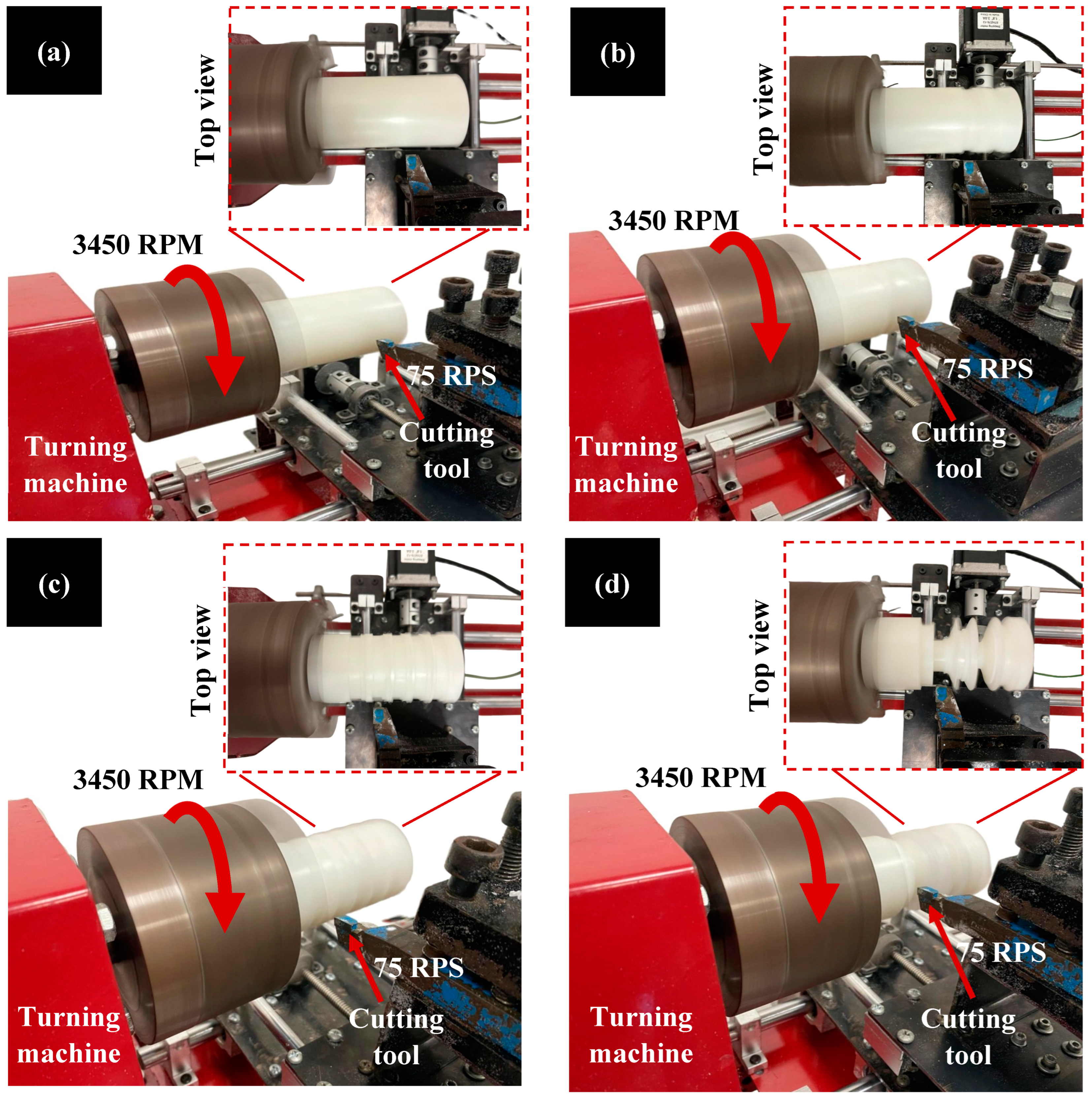
Figure 2 illustrates the sequential process of creating a high-precision Teflon component for the forearm joint of humanoid robots, specifically designed to enhance smooth rotational movement. The industrial turning machine operates at a fixed speed of 3450 RPM, and the cutting tool operates at a fixed 75 RPS, ensuring precise formation of the component. Figure 2a shows the Teflon material positioned and ready for machining. In Figure 2b, the cutting tool begins to shape the material, initiating contact and removing the initial layers. Figure 2c highlights the intermediate stage of shaping, with the cutting tool steadily advancing toward the final design. In Figure 2d, the desired Teflon part is completed and ready for use in the robot’s forearm joint, ensuring precision and durability in its movement. This automated approach underscores the importance of fault prediction and consistency in producing components critical to the functionality of advanced humanoid robots during mass production.

3.1. System Architecture of Time-to-Fault Prediction Framework

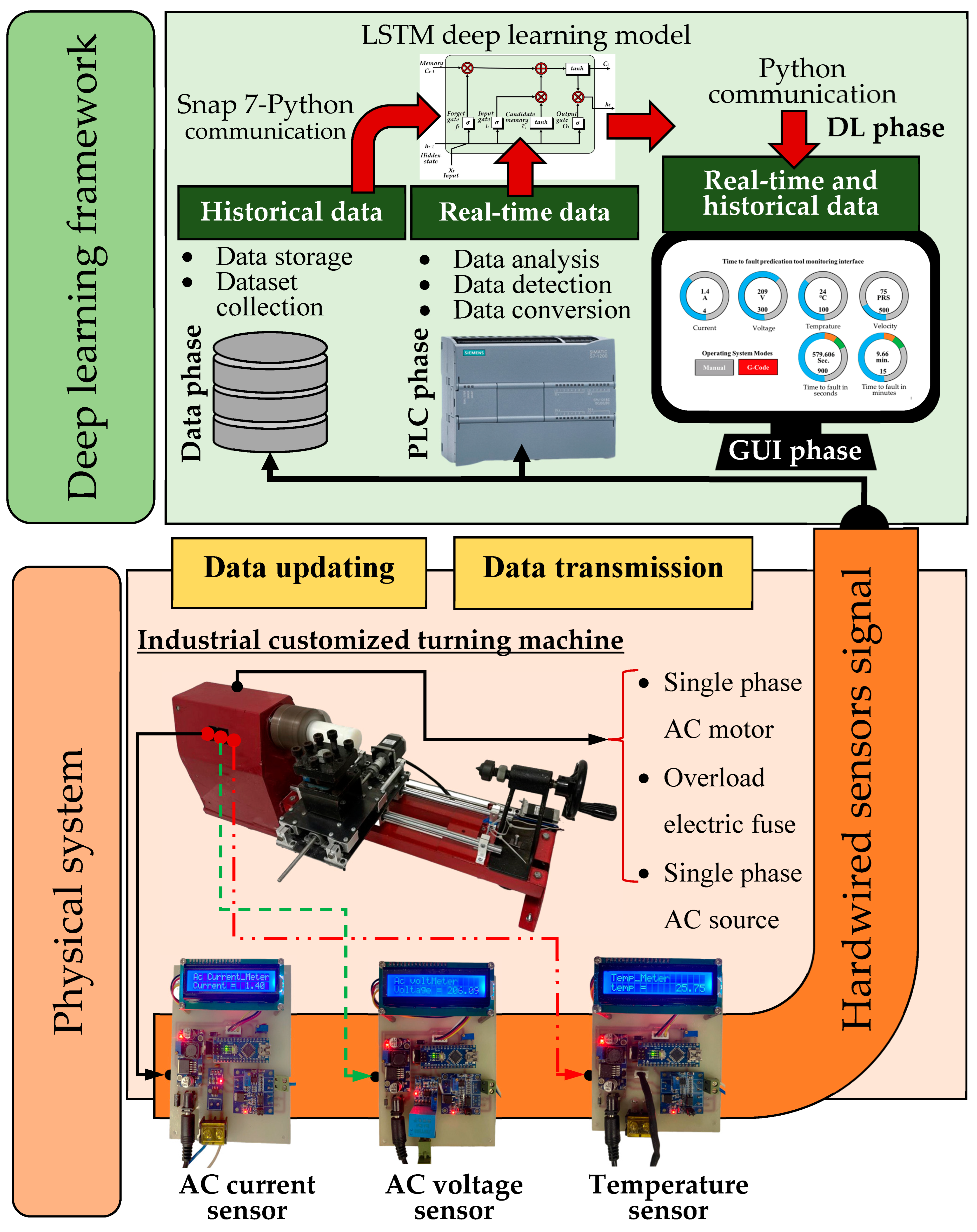
An overview of the proposed architecture for time-to-fault prediction in an actual industrial turning machine is presented in Figure 3. The architecture combines physical components with a deep learning framework to monitor, collect, analyze, and predict machine failure and performance. At the core of this architecture is the physical system, which includes the single-phase AC motor of an industrial turning machine. This motor is powered by a single-phase AC source and is protected by an overload fuse to ensure robust dataset development and operational stability. Hardwired sensors, including an AC current sensor, an AC voltage sensor, and a temperature sensor, continuously monitor the machine’s electrical and thermal parameters, capturing real-time data essential for predictive machine failures. These sensor data are transmitted to a programmable logic controller (Siemens AG (S7-1200 PLC): Munich, Germany) via a hardwired connection, ensuring accurate and reliable data capture.

The PLC phase analyzes, detects, and formats real-time data from the sensors for further processing. The PLC and human–machine interface (HMI) ensure that the data reflect the machine’s current operational status and is continuously updated. These data are then sent to the deep learning framework for advanced analysis.

The deep learning framework comprises several phases, including the data phase, the PLC phase, the DL phase, and the graphical user interface (GUI) phase. The data phase involves storing and managing historical data, which forms the basis for new dataset training and validating deep learning models. Historical data provide insights into long-term trends, while real-time data reflect the machine’s current state.

In the DL phase, an LSTM model is utilized to predict potential faults based on comparing both historical and real-time data. This model facilitates proactive maintenance by predicting time failures before they occur, minimizing unexpected downtimes. Python is used for communication within this phase, ensuring seamless data integration and model execution, with the Snap7 protocol enhancing communication between the PLC and the deep learning model.

The GUI phase provides users with an intuitive interface for monitoring machine performance. It visualizes historical and real-time data, displaying key metrics such as current, voltage, velocity, temperature, and time-to-fault predictions. This interface allows operators to interact with the system, observe trends, and make informed decisions based on the predictive insights generated by the deep learning model. Continuous data updating and transmission are critical in this architecture, ensuring that the deep learning model always works with the most current and relevant data. This continuous flow is essential for accurate fault time prediction, enabling the system to detect anomalies and predict potential failures effectively. By integrating real-time data acquisition, advanced data processing, sophisticated deep learning models, and user-friendly interfaces, this system architecture exemplifies the application of modern industrial automation technologies for proactive maintenance. It underscores the importance of data-driven decision-making in enhancing operational efficiency, reducing downtime, and extending the lifespan of industrial machinery.

3.2. Data Collection Based on Dataset Model Design

An advanced data collection system is specifically designed for predicting time-to-fault in a real industrial turning machine. This system employs a range of sensors and a robust control setup to meticulously monitor the machine’s performance, ensuring its reliable operation and safeguarding against potential failures. The main objective is to compile a detailed dataset that facilitates accurate fault predictions. At the core of the system is the S7-1200 PLC controller, which interfaces with an HMI and totally integrated automation portal (TIA Portal) V16 software through the TCP/IP protocol. This setup leverages historical data to develop a predictive model with high accuracy. The system is equipped with AC current, AC voltage, and temperature sensors, all connected using hardwired signals to track the operational parameters of a single-phase AC motor. These sensors continuously feed data into the system, allowing for real-time anomaly detection and fault prediction. An overload fuse is integrated into the system to develop a dataset without motor damage, while the dataset system model is designed to support comprehensive data collection and analysis. This enables proactive maintenance and minimizes downtime. Figure 4 provides a detailed system architecture, showcasing the approach for data collection of a time-to-fault prediction dataset in a real industrial turning machine. This system integrates advanced components and technologies to facilitate precise data collection, processing, and analysis, essential for predicting faults based on the time-to-failure and overload current relationship, as shown in Equation (1). The dataset is collected by examining time-to-failure alongside overload current across varying speeds on the x–y axis of a turning machine. The system architecture is meticulously divided into physical and digital components, thereby establishing a comprehensive framework for real-time monitoring and predictive maintenance. Electric motors play a pivotal role in numerous industrial and commercial applications, where their reliability is paramount for ensuring operational efficiency. To achieve optimal design and maintenance, it is crucial to understand the factors affecting motor lifespan. Mechanical and electrical stresses, particularly those induced by torque and current overloads, are significant determinants of motor durability. These stresses profoundly impact the motor’s time-to-failure. The relationship between time-to-failure, torque, and current overloads is described by the following equation [81,82,83,84,85,86]:

$$t_f \alpha {\displaystyle \frac{1}{{\tau }^n·{ I}^m}}$$

(1)

In this formula, $t_f$ denotes the motor’s time-to-failure, which decreases as both motor torque (τ) and motor current (I) increase. Torque introduces mechanical stress, leading to accelerated wear and a reduced lifespan. Concurrently, higher current generates increased electrical stress and heat due to I²R losses, which hastens insulation breakdown. The constants n and m are empirical values that reflect the motor’s design and material properties, determining its sensitivity to these stresses. Effectively managing these mechanical and electrical stresses is essential for enhancing motor reliability and extending its operational life in diverse applications.

At the core of the physical system is an industrial turning machine driven by a single-phase AC motor, powered by a single-phase AC source. To be able to develop a dataset of turning machines and protect the system from electrical faults like overcurrent that could lead to overheating and potential failure, an overload fuse is employed. This critical component ensures operational integrity by interrupting the power supply during excessive current flow, thereby maintaining system reliability and preventing AC motor damage. The system is managed by an S7-1200 PLC controller, which communicates with the TIA Portal software using the TCP/IP protocol. This setup allows for seamless programming, monitoring, and control of the turning machine, with the TIA Portal facilitating efficient system management through historical data acquisition and processing. An intuitive HMI provides operators with real-time data from sensors, historical records, and system status, crucial for monitoring machine performance and making informed decisions. The system integrates three types of sensors, including an AC current sensor, an AC voltage sensor, and a temperature sensor.

To ensure the robustness of the dataset, a novel calibration approach exploiting WGM technologies was employed [87,88,89,90,91,92,93,94]. The inherent high-quality factor of WGM resonators allows for the ultra-sensitive detection of minute changes in the surrounding medium, directly impacting the transmission spectrum. This characteristic was leveraged to calibrate the current, voltage, and temperature sensors, enhancing the accuracy and precision of the collected data. The resulting high-fidelity data, free from systematic errors introduced by traditional calibration methods, forms the foundation of a robust and reliable dataset for training and validating the predictive model.

To ensure accurate data acquisition, a rigorous calibration process is implemented using WGM-based optical sensors. The calibration procedure is based on correlating the shift in resonant frequencies of the WGM resonators with the corresponding physical parameters (current, voltage, and temperature). A predetermined calibration curve is constructed experimentally for each parameter by varying its value individually. The mathematical formulation used to convert the sensor’s output to electrical and thermal values takes the form of linear equations, with coefficients calculated from these experimental calibration curves. This enables precise and accurate data acquisition. To address missing data points, linear interpolation was employed, estimating missing values based on neighboring points. Segments were removed when the missing values were too long to be suitable for model training. Furthermore, a moving average filter with a five-point window was applied to mitigate noise, smoothing the signal by averaging data points and reducing random noise while preserving data patterns. A frequency analysis was performed on the signal before and after filtering to evaluate the noise reduction and ensure that it does not distort essential data patterns [87,88,89,90,91,92,93,94].

These sensors, connected through hardwired signals to the PLC device, are essential for data acquisition. The AC current sensor measures the motor’s electrical load, providing critical insights into current consumption and potential predictive faults. The AC voltage sensor monitors the voltage supplied to the motor, ensuring it remains within the specified range to avoid performance issues and faults. The temperature sensor tracks the thermal state of the motor, helping to identify thermal-related problems. Overload cylindrical miniature micro slow-blow fuse, a protective device, safeguards the dataset system model from electrical failures of the single-phase AC motor by automatically disconnecting the power supply in the event of an overload for developing dataset records without machine damage. The fuse rating is determined using the equation:

$$I_{fuse}=I_{rating}\times 1.25$$

(2)

where $I_{fuse}$ is the current rating of the fuse and $I_{rating}$ is the actual current drawn by the load.

Monitoring the motor’s performance is essential for fault prediction and ensuring smooth operation. Sensors provide real-time data on electrical and thermal parameters, which are transmitted to the PLC controller and then to the TIA Portal software and HMI log historical files. The historical data collected are crucial for developing accurate time-to-fault prediction models by identifying patterns and anomalies over time. Real-time data are also critical for creating predictive models, as they serve as input for deep learning algorithms designed for fault-time prediction. The system generates a comprehensive dataset by recording ten different speeds under manual and automatic operation, totaling around 18,567 records. The datasets are used to train and validate predictive deep learning models. This approach enables precise prediction of faults, enhancing the reliability and efficiency of the industrial turning machine.

To ensure the effectiveness and reliability of the proposed deep learning models, a robust data collection and preprocessing methodology is employed. Sensor data are collected using a customized industrial turning machine equipped with high-precision sensors, measuring current, voltage, and temperature at high frequencies and different machine velocities. The data were obtained through robust observations and validations under both manual and automatic operating conditions and at different speeds. To supplement the real sensor data and create realistic failure scenarios, a novel approach is employed to artificially generate time-to-failure data by systematically varying operational parameters. The collected data then underwent several techniques, beginning with the application of a linear interpolation to address missing values and removing big segments of missing data to ensure data continuity. Then, a moving average filter with a five-point window was applied to smooth noisy sensor signals. Finally, preprocessing (Min–Max normalization) is used to scale all features between 0 and 1, ensuring that all parameters contribute equally to the model’s learning process. These steps resulted in a robust and effective dataset suitable for training the deep learning models.

3.3. System Architecture of Time-to-Fault Prediction Using Deep Learning Models

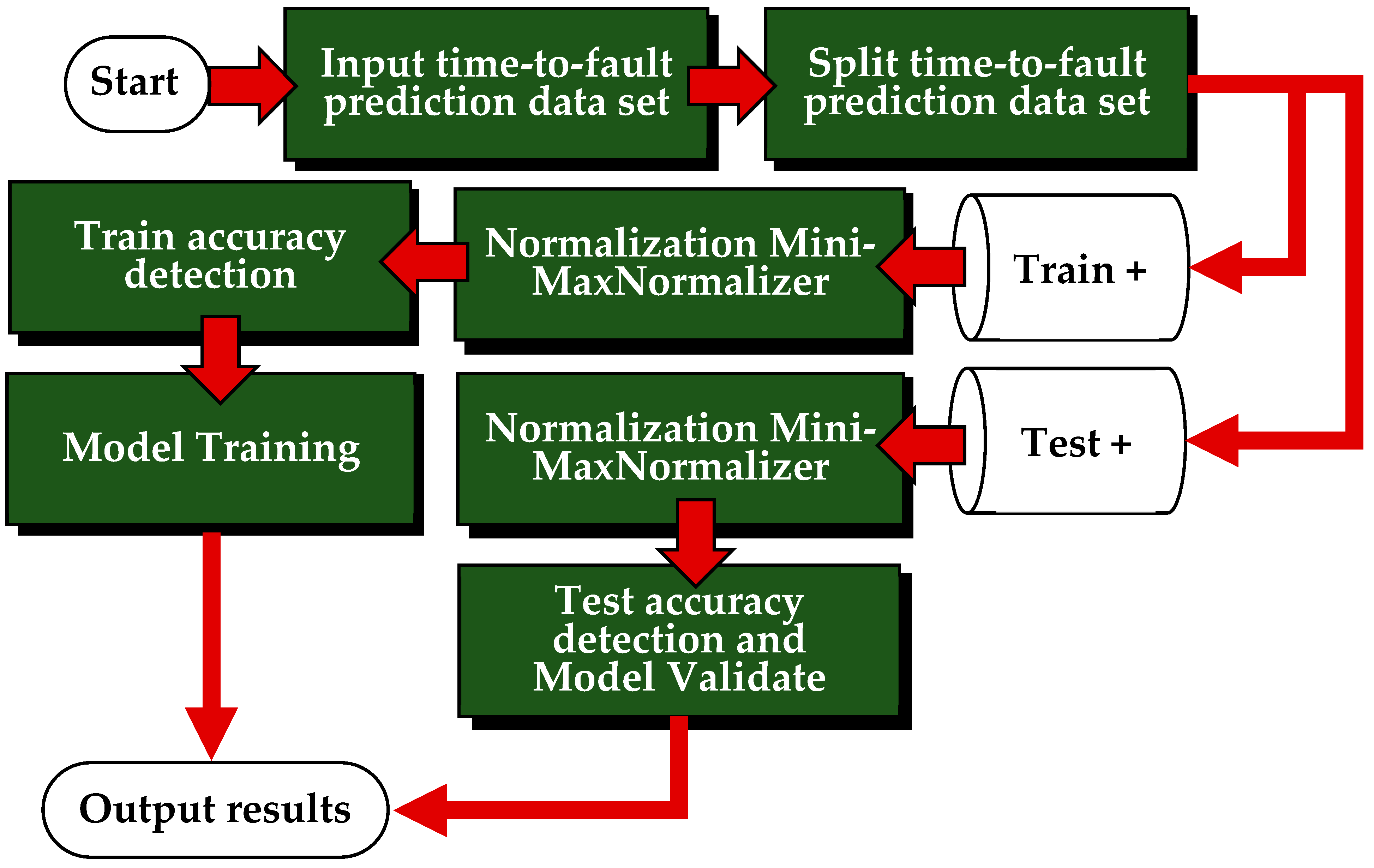
The system architecture presents the methodology for developing a time-to-fault prediction model using LSTM networks, as shown in Figure 5. Through this structured approach, an advanced predictive model is crafted, capable of delivering accurate machine failure predictions. This proactive framework enables timely maintenance interventions, effectively minimizing downtime and significantly boosting operational efficiency.

The provided system architecture outlines the development process for a time-to-fault prediction deep learning model using an LSTM for an industrial turning machine. This process encompasses several critical stages, including data input, preprocessing (including normalization), dataset splitting, model training with an LSTM, and validation. A detailed breakdown of each component and the equations involved is provided.

3.3.1. Data Preprocessing

Data preprocessing involves collecting historical data on turning machine operations, including faults and time-to-failure, and splitting the dataset into training and testing sets. Normalization is then applied to scale the features to a range between 0 and 1, ensuring all features contribute equally to the model’s learning process.

Input and Split Time-to-Fault Prediction Dataset

The initial step involves collecting a dataset containing historical data on real turning machine operations, including instances of faults and the corresponding time-to-failure. This dataset forms the foundation for training and testing the predictive model. To build a robust model, the dataset is split into two parts, including the training set and the testing set. The training set is used to train the model, while the testing set is reserved for evaluating its performance. This split helps assess the model’s ability to generalize to new, unseen data.

Normalization

Normalization is a preprocessing step that scales the features of the dataset to a specific range, typically between 0 and 1. This ensures that all features contribute equally to the model’s learning process, preventing any single feature from dominating due to its larger scale. The MinMaxNormalizer is commonly used for this purpose.

$$X \left(scaled\right)={\displaystyle \frac{X-min\left(x\right) }{max\left(x\right)-min\left(x\right)}}$$

(3)

where X (scaled) is the normalized value, X is the original value, min(x) is the minimum value in the dataset, and max(x) is the maximum value in the dataset.

3.4. Architectures of Deep Learning Models

Deep learning is a machine learning method that uses multilayered neural networks to identify patterns in large datasets. It automatically extracts features from raw data, making it suitable for tasks like image recognition, natural language processing, and time-series analysis. This approach is valuable across industries, improving over time as it processes more data.

3.4.1. LSTM Model

After completing the preprocessing of the dataset, a new compilation consisting of 18,567 observations has been generated, featuring six distinct attributes, including current sensor signal, voltage sensor signal, temperature sensor signal, velocity signal, operating system signal, and the estimated fault time. The first five attributes serve as input variables for training a LSTM network, while the estimated fault time acts as the output variable. The LSTM is specifically employed for predicting fault times in industrial turning machines. 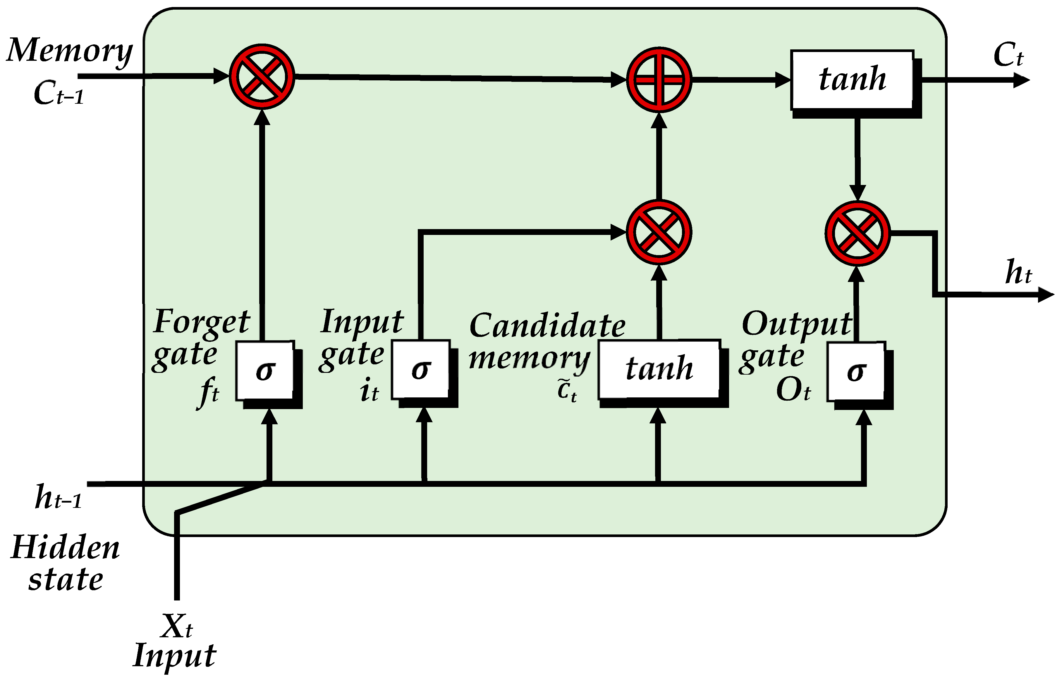Originally introduced by Hochreiter and Schmidhuber in 1997 [95], the LSTM architecture exhibits superior performance over traditional recurrent neural networks when managing sequential data. This advantage primarily stems from its integration of memory cells and gating mechanisms, enabling the LSTM to effectively handle long-term dependencies. Additionally, the architecture adeptly addresses the vanishing gradient problem, significantly enhancing the training process for deep models applied to sequential datasets. A comprehensive illustration of the architecture of a single LSTM unit is presented in Figure 6. To implement the LSTM network, the Keras library is used to construct a sequential model for regression tasks. The model begins with an LSTM layer that processes time-series data by learning temporal patterns and relationships inherent in the input. This layer outputs a single vector, as it is configured not to return sequences. A dense layer follows, introducing non-linearity to transform the extracted features, thereby enhancing the model’s ability to learn complex relationships. The final layer is another dense layer with a linear activation function, designed to generate a single continuous numerical output suitable for regression tasks. The model is compiled using the Adam optimizer, which facilitates efficient training through adaptive learning rate adjustments. The loss function employed is mean squared error (MSE), while MAE is used as an additional metric to monitor the model’s performance during training.

At each time step, an LSTM unit maintains both a hidden state and a memory state, which are regulated through three distinct gate mechanisms. The input gate determines the extent to which new information should be stored in the cell state. This gate evaluates the current input in conjunction with the previous hidden state, as expressed in the following equation:

$$i_t=\sigma (W_i · h_{t-1}-1,x_t]+b_i)$$

(4)

The candidate memory state, denoted as ${\tilde{C}}_t$, is computed using the same input and reflects new information that could potentially enhance the cell state. The formula for calculating the proposed cell state is as follows:

$${\tilde{C}}_t=tanh(W_C·[h_{t-1}-1,x_t]+b_C)$$

(5)

The forget gate regulates which information from the previous cell state is preserved and which should be discarded. This gate processes the previous hidden state in conjunction with the current input, expressed by the equation:

$$f_t=\sigma (W_f·[h_{t-1}-1,x_t]+b_f)$$

(6)

The cell state, a core component of the LSTM, is responsible for preserving long-term information. The update process is performed according to the following formula:

$$C_t=f_t\times C_{t-1}+i_t\times {\tilde{C}}_t$$

(7)

Finally, the output gate, which relies on both the previous hidden state and the current input, determines the output and the new hidden state through the following equations:

$$O_t=\sigma (W_o · h_{t-1}-1,x_t]+b_o)$$

(8)

$$h_t=O_t\times tanh\left(C_t\right)$$

(9)

This step-by-step mechanism enables LSTM units to effectively manage and update information over time, making them well-suited for tasks involving sequential data. The LSTM mechanism efficiently updates both hidden and cell states, enabling it to manage complex temporal dependencies in sequential data. The model architecture, summarized in

Table 1. LSTM model architecture details.

Block	Layers	Layer Size	Activation
Input block	Input layer	4	-
Hidden block 1	LSTM layer	64	-
	Dense layer	32	ReLU
Output block	Dense layer	1	Linear

, is divided into three main components. The input block includes an input layer with five features. Hidden block 1 comprises an LSTM layer with 64 units, followed by a dense layer with 32 units and ReLU activation, which captures both temporal dependencies and non-linear relationships. The output block consists of a dense layer with a single unit and a linear activation function to produce the regression output. Training parameters, outlined in

Table 2. LSTM model hyperparameters.

Parameter	Value
Batch size	32
Learning rate	Scheduled: initial = 0.001, factor = 0.5, Min = 1 × 10−5 (ReduceLROnPlateau)
Optimizer	Adam
Loss function	MSE
Metrics	MAE, RMSE, R2

, include a batch size of 32 to optimize gradient updates and a learning rate schedule controlled by the ReduceLROnPlateau method. The learning rate starts at 0.001 and decreases by a factor of 0.5, with a minimum value set at 1 × 10⁻⁵. The Adam optimizer ensures stable and efficient training. The model evaluates performance using MSE as the loss function and additional metrics such as MAE, RMSE, and R² score, providing a comprehensive assessment of prediction accuracy.

3.4.2. Comparing with Other Deep Learning Models

To evaluate the LSTM model’s performance comprehensively, comparisons are made with other deep learning techniques, including temporal convolutional network (TCN), autoencoder (AE), deep neural network (DNN), deep multilayer perceptron (Deep MLP), CNN, and GRU. These models are renowned for their classification and prediction capabilities across diverse domains [96,97,98,99]. By applying these methods to the same predictive task, a robust benchmark is established, highlighting the strengths and limitations of each approach.

TCN Model

This model uses a TCN for regression tasks. It starts with an input layer that defines the shape of the input data, consisting of four time steps, each with a single value. The first layer is a 1D convolutional layer (Conv1D), which applies filters to the input data to capture relationships across time. After this, a dropout layer is used to help prevent overfitting by randomly setting a portion of the input units to zero during training. Once the convolution and dropout operations are completed, the output is flattened using the flatten layer to transform the data into a one-dimensional vector, which is suitable for further processing by fully connected (dense) layers. The first dense layer, with ReLU activation, learns more complex patterns, while the second dense layer, with a single unit and linear activation, produces the final regression output. The model is trained using the Adam optimizer, which adjusts the learning rate to improve training efficiency. Mean squared error (MSE) is used as the loss function to minimize prediction error, and the model tracks MAE as an additional performance measure.

The model architecture is described in

Table 3. TCN model architecture details.

Block	Layers	Layer Size	Activation
Input block	Input layer	4	-
Hidden block 1	Conv1D layer	64	ReLU
	Dropout layer	-	-
	Flatten layer	-	-
	Dense layer	32	ReLU
Output block	Dense layer	1	Linear

, which begins with an input layer consisting of 4 units. It is followed by a convolutional layer with 64 filters and ReLU activation to capture patterns in the input data. A dropout layer, with no specified number of units, is applied to regularize the model, followed by flattening the data. The network continues with a dense layer of 32 units, using ReLU activation, and ends with a dense layer with 1 unit and linear activation for the regression output.

Table 4. TCN model hyperparameters.

Parameter	Value
Batch size	32
Learning rate	Scheduled: initial = 0.001, factor = 0.5, min = 1 × 10−5 (ReduceLROnPlateau)
Optimizer	Adam
Loss function	MSE
Metrics	MAE, RMSE, R2

presents the hyperparameters used during training. The batch size is set to 32, and the learning rate starts at 0.001, following a scheduled reduction pattern managed by the ReduceLROnPlateau callback. This callback reduces the learning rate by half if no improvement is observed, with a minimum learning rate of 1 × 10⁻⁵. The performance of the model is evaluated using MAE, RMSE, and R², providing a comprehensive view of its accuracy.

AE Model

The AE model is designed for regression tasks. It starts with an input layer that defines the shape of the input data, consisting of four features. The encoder portion of the model consists of several dense layers that gradually reduce the dimensionality of the input data, extracting progressively more abstract representations. The final encoder layer, known as the bottleneck, represents the compressed form of the data. The decoder part reconstructs the data by expanding it through dense layers, bringing it back to the original size, and ultimately generating the regression output with a single unit and a linear activation function in the final layer.

The model is trained using the Adam optimizer, with MSE as the loss function, which aims to minimize prediction errors. MAE is tracked as an additional performance measure. The autoencoder structure is designed to learn a compact representation of the input data while preserving the ability to predict continuous values.

Table 5. AE model architecture details.

Block	Layers	Layer Size	Activation
Input block	Input layer	4	-
Hidden block 1	Dense layer	64	ReLU
	Dense layer	32	ReLU
	Dense layer	16	ReLU
	Dense layer	8	ReLU
Bottleneck	Dense layer	4	ReLU
Decoder block	Dense layer	8	ReLU
	Dense layer	16	ReLU
	Dense layer	32	ReLU
	Dense layer	64	ReLU
Output block	Dense layer	1	Linear

and

Table 6. AE model hyperparameters.

Parameter	Value
Batch size	32
Learning rate	0.001
Optimizer	Adam
Scheduled learning rate	Initial = 0.001, factor = 0.2, min = 0.0001 (ReduceLROnPlateau)
Loss function	MSE
Metrics	MAE, RMSE, R2

describe the model’s architecture and hyperparameters. The encoder progressively reduces the input dimensions through dense layers with sizes 64, 32, 16, and 8 units, using ReLU activation at each step. The bottleneck layer, with 4 units, represents the compressed representation. The decoder mirrors the encoder’s structure, expanding the dimensions through dense layers of 8, 16, 32, and 64 units, all using ReLU activation. The final output layer is a dense layer with 1 unit and a linear activation function, producing continuous values.

The model uses a batch size of 32, with an initial learning rate of 0.001. The learning rate is scheduled using the ReduceLROnPlateau callback, reducing it by a factor of 0.2 if validation loss plateaus, with a minimum learning rate set to 0.0001. During training, the model is evaluated using MAE, RMSE, and R² to assess its performance.

DNN Model

This model defines a DNN for regression tasks. It starts with an input layer that specifies the shape of the input data, consisting of four features. The network includes three dense layers, each followed by ReLU activation. These layers progressively learn more complex representations of the input data, with the first two hidden layers having an increasing number of neurons, while the third layer introduces moderate complexity. To reduce overfitting, a dropout layer is applied after the hidden layers, randomly setting a fraction of the units to zero during training. The output layer consists of a dense layer with a single unit and linear activation, suitable for regression tasks.

The model is trained using the Adam optimizer with a learning rate of 0.001 and uses MSE as the loss function. The performance is evaluated by tracking MAE in addition to MSE, and other metrics such as RMSE and R² are used for a more detailed assessment of model accuracy.

The DNN model described in

Table 7. DNN model architecture details.

Block	Layers	Layer Size	Activation
Input block	Input layer	4	-
Hidden block 1	Dense layer	128	ReLU
Hidden block 2	Dense layer	64	ReLU
Hidden block 3	Dense layer	32	ReLU
Regularization	Dropout layer	-	-
Output block	Dense layer	1	Linear

consists of an input layer with 4 features, followed by 3 hidden layers with 128, 64, and 32 neurons, respectively, all utilizing ReLU activation. After the hidden layers, a dropout layer with a rate of 0.2 helps prevent overfitting. The output layer has a single neuron with linear activation, suitable for regression tasks.

Table 8. DNN model hyperparameters.

Parameter	Value
Batch size	32
Learning rate	0.001
Optimizer	Adam
Loss function	MSE
Metrics	MAE, RMSE, R2
Dropout rate	0.2 (Dropout for regularization)
Learning rate schedule	ReduceLROnPlateau (monitor = val_loss, factor = 0.2, min LR = 0.0001)

outlines the hyperparameters, which include a batch size of 32 and the Adam optimizer with an initial learning rate of 0.001. The training process is enhanced by a learning rate schedule using the ReduceLROnPlateau callback, which reduces the learning rate by a factor of 0.2 if the validation loss does not improve, with a minimum learning rate of 0.0001.

Deep MLP Model

An MLP is designed for regression tasks. The model starts with an input layer that specifies the shape of the input data, which includes four features. The first dense layer uses ReLU activation and includes L2 regularization, a technique that helps prevent overfitting by penalizing large weights. Batch normalization is applied to standardize the activations, which improves convergence and training speed. Additionally, a dropout layer is used to reduce overfitting by randomly setting a portion of the input units to zero during training.

This pattern repeats for two more dense layers, each with ReLU activation, L2 regularization, batch normalization, and dropout. The final output layer consists of a dense unit with a linear activation function, providing the regression output. The model is compiled using the Adam optimizer, with mean squared error (MSE) as the loss function to minimize prediction errors. The model also tracks the MAE to evaluate its performance. This architecture is designed to learn complex patterns from the data while controlling overfitting through regularization, batch normalization, and dropout techniques.

As shown in

Table 9. Deep MLP model architecture details.

Block	Layers	Layer Size	Activation
Input block	Input layer	4	-
Hidden block 1	Dense layer	128	ReLU
	Batch normalization	-	-
	Dropout	-	-
Hidden block 2	Dense layer	128	ReLU
	Batch normalization	-	-
	Dropout	-	-
Hidden block 3	Dense layer	128	ReLU
	Dropout	-	-
Output block	Dense layer	1	Linear

and

Table 10. Deep MLP model hyperparameters.

Parameter	Value
Batch size	32
Learning rate	Scheduled: initial = 0.001, factor = 0.5, min = 1 × 10−5 (ReduceLROnPlateau)
Optimizer	Adam
Loss function	MSE
Metrics	MAE, RMSE, R2

, the MLP model is structured into four main blocks, including the input block, three hidden blocks, and the output block. The input block includes the input layer with four features, followed by three hidden blocks. Each hidden block contains a dense layer with 128 units and ReLU activation. Each hidden block also includes batch normalization to stabilize training and a dropout layer with a rate of 0.001 to further prevent overfitting. The output block consists of a single dense layer with one unit and a linear activation function, suitable for regression tasks.

The model is compiled with the Adam optimizer and uses a learning rate schedule. The initial learning rate is 0.001, with a reduction factor of 0.5 and a minimum learning rate of 1 × 10⁻⁵. The performance is evaluated using MSE, MAE, RMSE, and R² metrics, and the model is trained with a batch size of 32.

CNN Model

The CNN model is also designed for regression tasks. It starts with an input layer that specifies the shape of the input data, consisting of four features. The first CNN block applies a Conv1D layer with batch normalization, ReLU activation, and MaxPooling1D to extract important features from the input sequence. A dropout layer follows to reduce overfitting.

The second CNN block is similar, but uses a larger kernel size and includes reduced pooling, followed again by dropout. After this, the output is flattened into a 1D array to feed into the MLP block. The MLP block includes a dense layer with L2 regularization to learn complex patterns from the CNN features. Batch normalization, ReLU activation, and dropout are applied to help prevent overfitting.

The final output layer is a dense unit with a linear activation function to generate continuous regression outputs. The model is compiled using the Adam optimizer with mean squared error (MSE) as the loss function and MAE as an additional evaluation metric.

As shown in

Table 11. CNN model architecture details.

Block	Layers	Layer Size	Activation
Input block	Input layer	(4, 1)	-
Hidden block 1	Conv1D layer	512 (kernel: 2)	ReLU
	Batch normalization	-	-
	MaxPooling1D	Pool size: 2	-
	Dropout layer	-	-
Hidden block 2	Conv1D layer	512 (kernel: 4)	ReLU
	Batch normalization	-	-
	MaxPooling1D	Pool size: 2	-
	Dropout layer	-	-
MLP block	Dense layer	1024	ReLU
	Batch normalization	-	-
	Dropout layer	-	-
Output block	Dense layer	1	Linear

and

Table 12. CNN model hyperparameters.

Parameter	Value
Batch size	32
Learning rate	Scheduled: initial = 0.001, factor = 0.5, min = 1 × 10−5 (ReduceLROnPlateau)
Optimizer	Adam
Loss function	MSE
Metrics	MAE, RMSE, R2

, the CNN model architecture consists of multiple layers designed to process time-series data with a shape of (4, 1) as the input. The first block applies a Conv1D layer with 512 filters and a kernel size of 2, followed by batch normalization, ReLU activation, max pooling with a pool size of 2, and a dropout layer. The second block applies a Conv1D layer with 512 filters and a kernel size of 4, followed by batch normalization, ReLU activation, max pooling, and another dropout layer.

The output of these blocks is flattened and passed through an MLP block. The MLP block consists of a dense layer with 1024 units, batch normalization, ReLU activation, and dropout. The final output layer is a dense unit with one unit and a linear activation function. The model is trained using a batch size of 32, and the learning rate schedule starts at 0.001 with a reduction factor of 0.5 and a minimum learning rate of 1 × 10⁻⁵. The model is evaluated using MSE, MAE, RMSE, and R².

GRU Model

The GRU model is designed for regression tasks, specifically for sequential data. The model begins with a GRU layer, which processes the sequential data and returns the final output of the sequence, using 64 units to capture temporal dependencies. This layer is followed by a dense layer with ReLU activation, introducing non-linearity and helping the model learn more complex relationships.

The final output layer is another dense layer with a linear activation function, providing a continuous value for regression tasks. The model is compiled with the Adam optimizer, using mean squared error (MSE) as the loss function to minimize prediction errors and MAE as an additional evaluation metric.

The architecture of the GRU model, as shown in

Table 13. GRU model architecture details.

Block	Layers	Layer Size	Activation
Input block	GRU layer	64	-
Hidden block 1	Dense layer	32	ReLU
Output block	Dense layer	1	Linear

and

Table 14. GRU model hyperparameters.

Parameter	Value
Batch size	32
Learning rate	Scheduled: initial = 0.001, factor = 0.5, min = 1 × 10−5 (ReduceLROnPlateau)
Optimizer	Adam
Loss function	MSE
Metrics	MAE, RMSE, R2

, begins with an input layer that expects four time steps, with one feature per step. The first hidden block consists of a GRU layer with 64 units, followed by a dense layer with 32 units and ReLU activation. The output block contains a final dense layer with one unit and a linear activation function for regression.

The batch size is set to 32, and the learning rate follows a scheduled reduction pattern, starting at 0.001, with a reduction factor of 0.5 and a minimum value of 1 × 10⁻⁵, controlled by the ReduceLROnPlateau callback. The optimizer is Adam, and the loss function used is MSE. The performance of the model is evaluated using MAE, RMSE, and R² metrics.

3.5. Performance Evaluation Metrics

All training validations conducted in this study utilized the RMSE performance index. This metric represents the standard deviation of the differences between the estimated values and the predicted values [21]. The RMSE is calculated using the following equation [20,21,70]:

$$RMSE=\sqrt{{\displaystyle \frac{1}{n}} · {\sum }_{i=1}^n{( x_{i }^{\prime }-x_i )}^2 }$$

(10)

Here, n denotes the number of observations being compared, $x_{i }^{\prime }$ is the value of the $i$th element in the predicted results vector, and $x_i$ is the corresponding value from the test dataset.

The MAE quantifies the average size of errors in a set of predictions without considering whether the errors are positive or negative. It is computed as the mean of the absolute differences between the actual values and the predicted values:

$$MAE={\displaystyle \frac{1}{n}} · {\sum }_{i=1}^n| y_i-{\hat{y}}_i |$$

(11)

In this equation, $n$ represents the total number of data points, $y_i$ is the actual value, and ${\hat{y}}_i$ is the predicted value.

The coefficient of determination, denoted as $R^2$, measures the extent to which the model accounts for the variability in the target variable. The scale ranges from 0 to 1, with a value of 1 representing complete predictive accuracy:

$$R^2=1-{\displaystyle \frac{{\sum }_{i=1}^n({y_i-{\hat{y}}_i)}^2}{{\sum }_{i=1}^n({y_i-\overline{y})}^2}}$$

(12)

In this formula, $n$ represents the number of data points, $y_i$ denotes the actual value, ${\hat{y}}_i$ is the predicted value, and $\overline{y}$ is the mean of the actual values.

4. Results and Discussion

Time-to-fault prediction for industrial turning machines is achieved using advanced techniques from deep learning, including LSTM, GRU, CNN, Deep-MLP, DNN, AE, and TCN in the deep learning models. Extensive training on a novel fault time prediction dataset and careful tuning of the models’ parameters have enabled these deep learning models to achieve high performance metrics, including high prediction performance and reliability. Among these techniques, the LSTM model stands out for its exceptional effectiveness in accurately predicting the time until faults occur in the industrial turning machine. The LSTM’s performance is compared using metrics such as MAE, RMSE, and R² with other deep learning models.

4.1. Deep Learning Techniques

Deep learning uses neural networks to automatically learn patterns from large datasets, improving prediction accuracy and classification. Unlike traditional machine learning, which requires manual feature extraction, deep learning models automatically identify the relevant features from raw data. This ability is especially useful for complex tasks like fault prediction, as deep learning models can handle various types of data and adapt to complex relationships within it.

A comparison of several deep learning models is presented in

Table 15. Comparison of performance metrics for predictive deep learning models.

Model	TCN	AE	DNN	MLP	CNN	GRU	LSTM
MAE	2.56	1.84	1.62	1.44	0.93	0.87	0.83
RMSE	3.97	2.71	2.6	1.89	1.52	1.79	1.62
R2	0.99	0.99	0.99	0.99	0.99	0.99	0.99

, including LSTM, GRU, CNN, Deep-MLP, DNN, AE, and TCN, based on three performance metrics (MAE, RMSE, and R²). These metrics are crucial for evaluating how well the models predict fault time. As shown in Figure 7, the LSTM model performs the best, with the lowest MAE of 0.83, indicating high precision in predictions. It also achieves a low RMSE of 1.62, further confirming its ability to minimize prediction errors. The GRU model, another recurrent neural network, also performs well, with an MAE of 0.87 and RMSE of 1.79. This suggests that GRU and LSTM have similar performance levels. The CNN model also performs well, with an MAE of 0.93 and the lowest RMSE of 1.52, showing its strength in capturing complex data patterns.

In contrast, the Deep-MLP model shows higher error rates, with an MAE of 1.44 and an RMSE of 1.89, suggesting it may not be the best choice for this particular task. The TCN model, with an MAE of 2.56 and RMSE of 3.97, shows higher errors, suggesting that it may not be as effective for time-to-fault prediction. The AE model has an MAE of 1.84 and RMSE of 2.71, performing between Deep-MLP and the stronger models. The DNN model, with an MAE of 1.62 and RMSE of 2.6, is competitive but still lags behind the top-performing models like LSTM and GRU.

Despite these differences in error rates, all models achieve an impressive R² value of 0.99, meaning they explain 99% of the variance in the data. This shows that all models have a strong ability to predict fault time, but LSTM performs the best in terms of minimizing errors. Overall, while all models are accurate, LSTM is the most accurate and reliable, followed closely by GRU and CNN. The Deep-MLP, DNN, AE, and TCN models demonstrate lower performance compared to the LSTM. This highlights the superior performance of the LSTM model.

The developed time-to-fault prediction system offers substantial real-world implications for industrial manufacturing. By accurately predicting faults with a 10 min lead time, the proposed framework allows operators to perform timely maintenance, minimizing unplanned downtime. This proactive approach can lead to significant cost savings by reducing repair costs and lost production time, as well as extending the lifespan of the machinery. For instance, if machine downtime costs USD 500 per hour, reducing unplanned stoppages can generate considerable savings. Furthermore, the proposed system enhances productivity by enabling smoother, continuous production and ensuring that maintenance is scheduled during non-critical hours, optimizing resource utilization and machine performance. By maintaining machines in their optimal condition for extended periods, the system increases efficiency and reduces production process disruptions. Examples of these practical benefits, supported by real industrial data, are detailed further in the following discussion.

4.2. Time-to-Fault Prediction Based on Deep Learning Models Using GUI

The GUI phase for time-to-fault prediction in industrial turning machines provides real-time monitoring of key inputs and output, including current, voltage, temperature, velocity, operating system type, and time-to-fault prediction. These inputs are essential for evaluating machine health and detecting potential faults early. The dashboard is divided into six sections, including current, voltage, temperature, velocity, operating system, and time-to-fault prediction. Real-time measurements for current, voltage, and temperature are displayed, while velocity and operating system values are user-selected. The time-to-fault prediction section outputs the estimated time-to-failure, ranging from 1.6 min (99 s) to 10 min (580 s). Three velocities from a set of ten (ranging from 75 to 500 pulses/s) are used for model validation. Ten scenarios are implemented to create the fault prediction dataset of 18,567 records, with three discussed in detail and one scenario validated. This proactive system allows for timely maintenance, minimizing downtime and maintenance costs, and optimizing operational efficiency and safety.

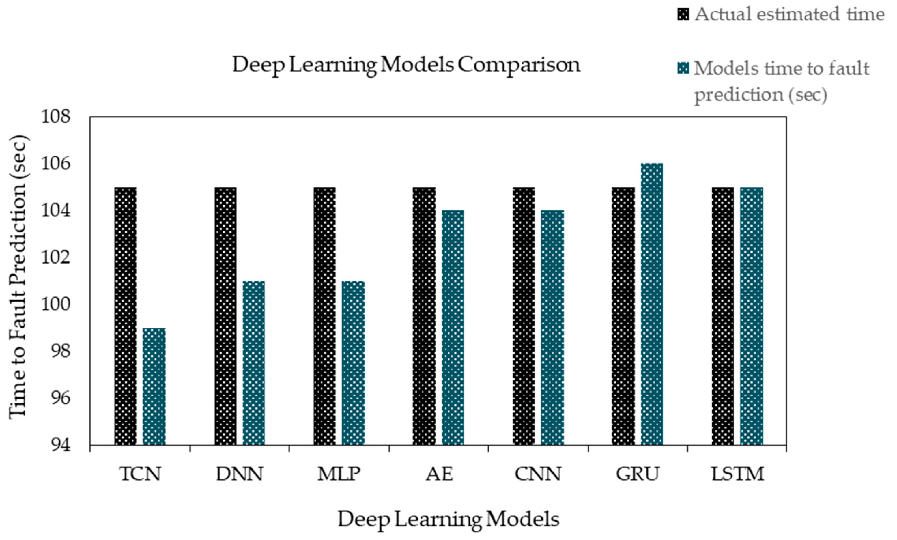
4.2.1. First Scenario of Time-to-Fault Prediction (Velocity: 500 Pulses/s)

The performance of different deep learning models in predicting the fault time in the first scenario is compared in

Table 16. Comparison of actual and predicted time-to-fault for deep learning models in the first scenario.

Model	TCN	DNN	MLP	AE	CNN	GRU	LSTM
Actual estimated time	105	105	105	105	105	105	105
Model time-to-fault prediction (sec)	99	101	101	104	104	106	105

. The evaluation compares the actual estimated fault time with the predicted fault time from each model. Accurately predicting the fault time is essential for effective predictive maintenance. The actual estimated fault time is 105 s for all models, while the predicted fault times vary across the models.

The Deep-MLP model predicts the fault time at 101 s, which is slightly earlier than the actual estimate, suggesting it tends to overpredict. The CNN model predicts 104 s, very close to the actual time, showing high accuracy. The TCN model predicts the fault time at 99 s, underestimating the actual time by 6 s, while the DNN model predicts 101 s. The AE model predicts 104 s, similar to the CNN model. The GRU model predicts 106 s, slightly overestimating the fault time by 1 s, while the LSTM model predicts 105 s, matching the actual time exactly.

While all models perform differently, the LSTM model is the most accurate, matching the actual fault time perfectly. The GRU, CNN, and AE models also perform well, with minimal deviation from the actual time. The other models, such as Deep-MLP, DNN, and TCN, show some deviation, indicating areas for improvement. This highlights the importance of selecting the appropriate deep learning model for predictive fault time tasks. The LSTM model stands out as the preferred choice due to its precise predictions, as shown in Figure 8.

4.2.2. Second Scenario of Time-to-Fault Prediction (Velocity: 250 Pulses/s)

The performance of seven deep learning models in predicting fault time is compared in

Table 17. Comparison of actual and predicted time-to-fault for deep learning models in the second scenario.

Model	TCN	DNN	MLP	AE	CNN	GRU	LSTM
Actual estimated time	193	193	193	193	193	193	193
Model time-to-fault prediction (sec)	192	190	188	188	191	192	192

. The actual fault time is consistently 193 s, while the predicted fault time differs for each model. The MLP model predicts 188 s, underestimating the actual time. The CNN model predicts 191 s, very close to the actual time. The DNN model predicts 190 s, slightly underestimating the time, while the AE model predicts 188 s, underestimating by 5 s. The TCN, GRU, and LSTM models predict 192 s, showing minimal deviation and matching the actual time closely, resulting in the highest accuracy.

Figure 9 shows that TCN, GRU, and LSTM are the most accurate models, with DNN and CNN also performing well. However, the MLP and AE models require further refinement. This emphasizes the importance of selecting the appropriate deep learning model for predictive fault detection, with LSTM standing out for its precision.

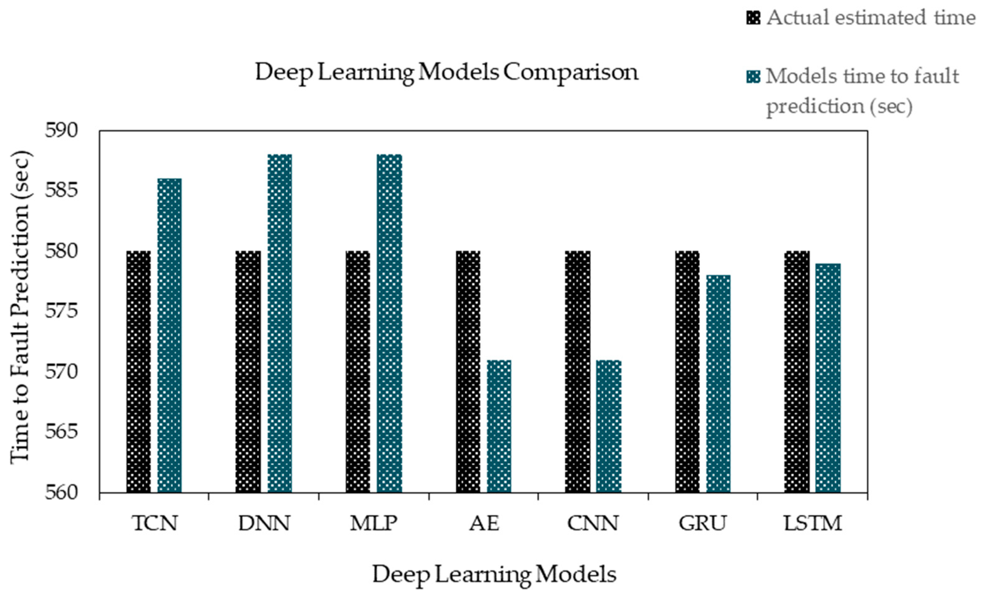
4.2.3. Third Scenario of Time-to-Fault Prediction (Velocity: 75 Pulses/s)

The predictions of fault time from various deep learning models, with the actual fault time being 580 s, are compared in

Table 18. Comparison of actual and predicted time-to-fault for deep learning models in the third scenario.

Model	TCN	DNN	MLP	AE	CNN	GRU	LSTM
Actual estimated time	580	580	580	580	580	580	580
Model time-to-fault prediction (sec)	586	588	588	571	571	578	579

. The Deep-MLP model overestimates the fault time by 8 s, while both the CNN and AE models underestimate it by 9 s. The TCN model predicts 586 s, slightly overestimating the time by 6 s. Similarly, the DNN model predicts 588 s, overestimating the fault time by 8 s. The GRU model predicts 2 s below the actual time, while the LSTM model provides the closest prediction, estimating just 1 s lower than the actual fault time.

As shown in Figure 10, the LSTM model provides the most accurate prediction, followed closely by the GRU model. The CNN and AE models show slight underestimations, while the TCN, DNN, and Deep-MLP models slightly overestimate the fault time. This reinforces the superior accuracy of the LSTM model in predicting fault time, making it the most reliable model for fault prediction.

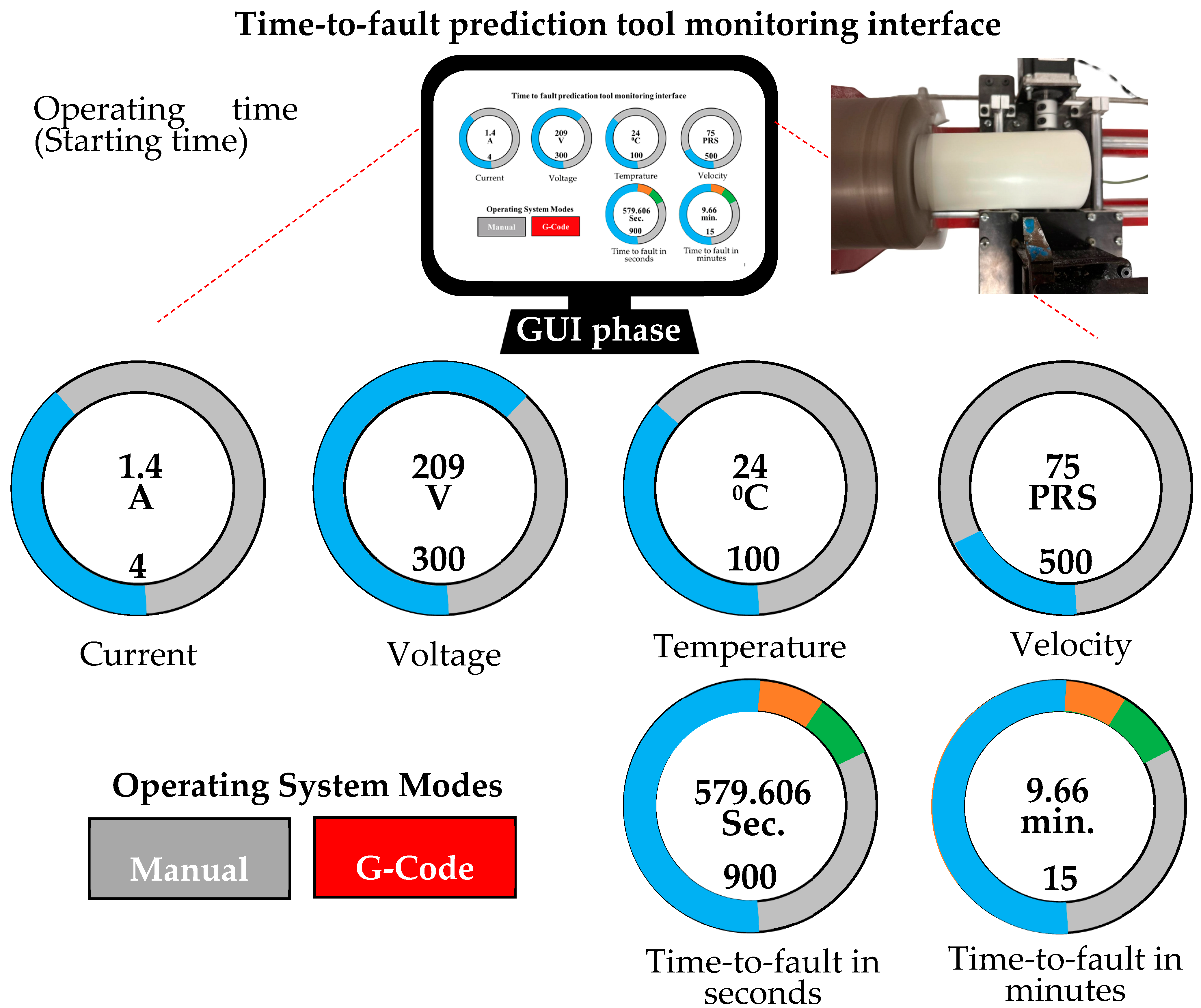
4.2.4. Validation of Third Scenario Prediction in Deep Learning Framework

The time-to-fault prediction tool is shown in Figure 11, a system used to monitor and predict machine failure for industrial machinery, focusing on the initial stage of the third scenario. The interface displays key operational parameters, including current, voltage, temperature, and velocity, using circular gauges that provide a clear and intuitive visualization of each parameter’s current state. In the top row, the gauges indicate that the machinery is operating at 1.4 amps for current, 209 volts for voltage, 24 degrees for temperature, and 75 pulses/s for velocity. Each gauge is color-coded, reflecting the current values in relation to their maximum operating limits, allowing operators to quickly assess whether any parameter is approaching a critical threshold. These data are crucial for predicting potential faults, enabling proactive maintenance, and minimizing unplanned downtime.

Additionally, the interface features two operating system modes, including manual and G-Code, highlighted in gray and red, respectively. The selected mode, G-Code, suggests that the machinery is currently operating in an automated, programmable mode, which is common in turning machine systems. The interface provides a real-time fault prediction, displaying both the time-to-fault in seconds (around 579.606 s) and minutes (around 9.66 min). This predictive information is vital for operators to take timely action to either halt the machine or initiate maintenance protocols, reducing the risk of damage and ensuring continuous, efficient operation. The circular gauges for the fault time include color segments such that the blue color represents the exact value, the green color represents +10% of the exact value, and the orange color represents −10% of the exact value because of fuse tolerances, further aiding quick decision-making. Overall, this monitoring tool serves as a comprehensive interface that combines real-time operational data with fault prediction capabilities, facilitating efficient maintenance planning and enhancing the reliability of industrial machinery. The system’s design emphasizes clarity and usability, ensuring that operators can easily interpret the data and take necessary actions to maintain optimal performance.

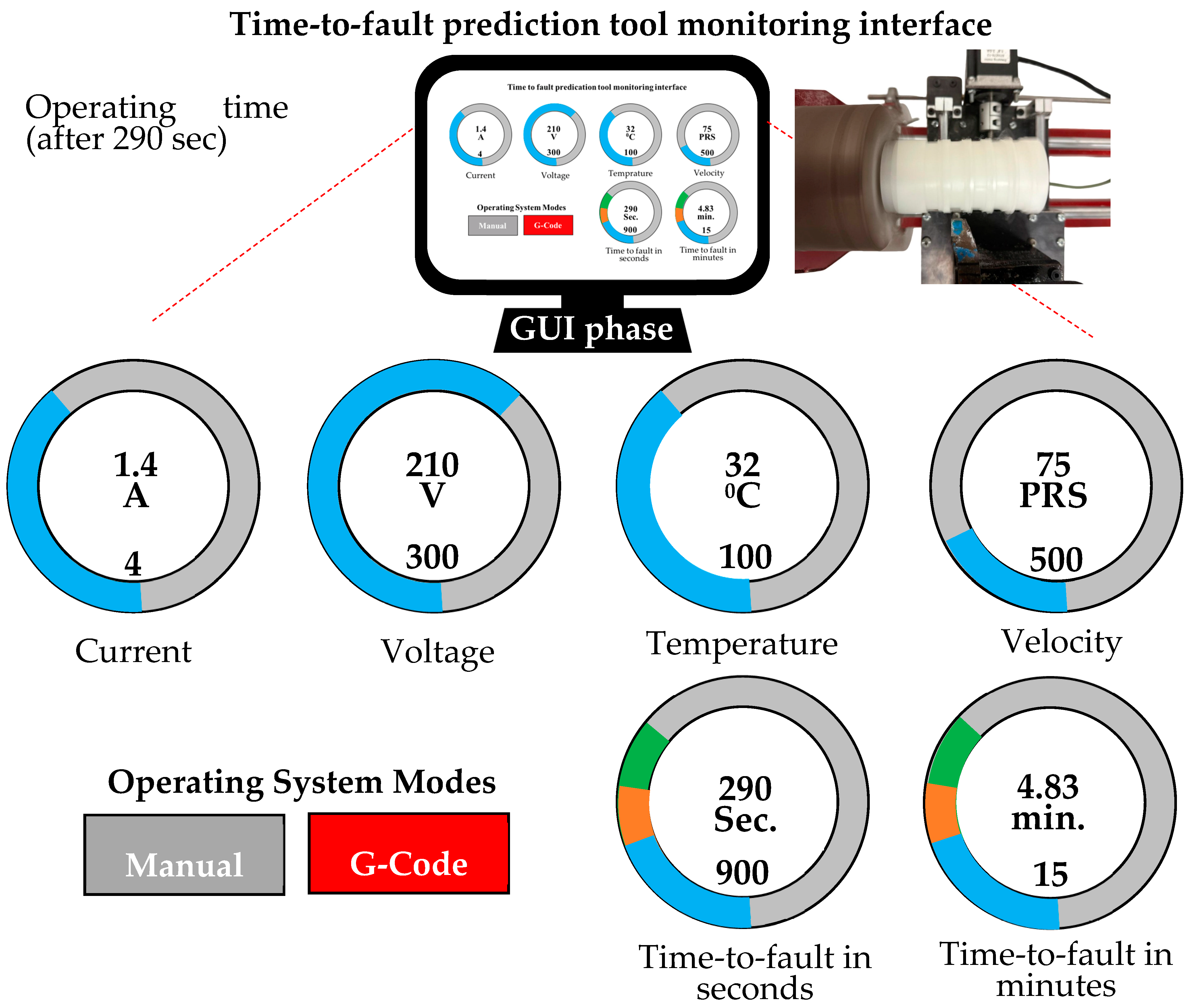
The time-to-fault prediction tool monitoring interface is presented in Figure 12, de-signed for real-time monitoring and predictive failure of industrial machinery during the intermediate stage of the third scenario. It presents key parameters, including current (1.4 amps), voltage (210 volts), temperature (32 degrees), and velocity (75 pulses/s) through color-coded gauges for quick assessment. It also indicates a time-to-fault of approximately 290 s (4.83 min), allowing for timely maintenance. The design emphasizes clarity and functionality to aid operators in optimizing machinery performance.

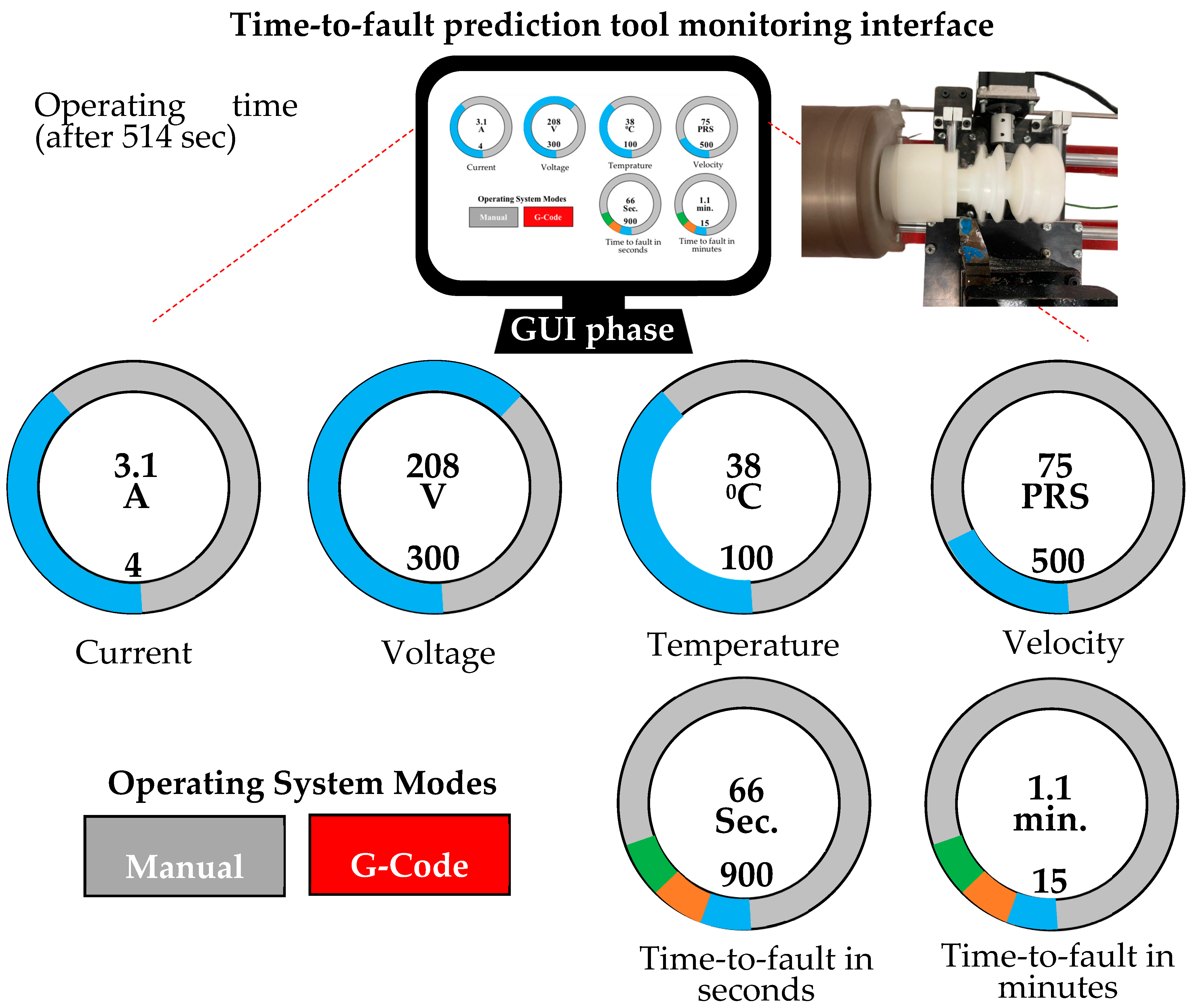
The monitoring interface at the last stage of the third scenario is presented in Figure 13. It features color-coded circular gauges displaying key metrics, including current (3.1 amps), voltage (208 volts), temperature (38 degrees), and velocity (75 pulses/s). It also shows real-time fault prediction data, indicating a time-to-fault of about 66 s (1.1 min) to support timely maintenance. The design prioritizes clarity and functionality to improve decision-making and optimize machinery performance.

5. Challenges and Limitations

The development of an advanced predictive framework for fault time prediction in industrial turning machines faced several significant challenges. Ensuring the dataset’s accuracy and comprehensiveness required precise sensors to capture key parameters such as current, voltage, and temperature under varying operational conditions. Additionally, integrating complex factors like overload currents and cutting tool speeds further complicated the process. Implementing the enhanced LSTM model added another layer of difficulty, as it required extensive tuning, real-time monitoring, and the management of high computational demands to outperform other deep learning models. Predicting failures early within a critical 10 min also posed significant challenges, requiring highly sensitive data to identify early signs of failure. Despite the promising results, several limitations need to be addressed to improve the framework’s generalizability and real-world applicability:

• The model assumes that protective devices, such as fuses, will operate reliably. However, environmental and operational variations, like temperature changes and power supply instability, can impact fuse performance, leading to inaccurate failure predictions. This highlights the need for improved protective devices and further research into fuse behavior under different conditions.
• While the LSTM model has shown strong performance, exploring alternative deep learning models with potentially higher accuracy presents challenges such as increased complexity, larger dataset requirements, and more intensive fine-tuning. These factors may complicate real-time deployment in industrial settings.
• The dataset used is limited to specific types of machines and faults, which may limit the framework’s generalizability to other machines and fault types.

6. Conclusions

Industry 4.0 aims to enhance operational efficiency by leveraging smart technologies, and predictive maintenance plays a pivotal role in achieving this goal. This study presents an approach for predicting machine failures in industrial machines using a robust dataset derived from sensor data (current, voltage, and temperature) calibrated optically based on the typical WGM technologies. The dataset is created from actual sensor readings taken during motion and cutting operations, with the aim of predicting failures within 10 min. This approach utilizes an enhanced LSTM model, which was selected for its strong generalization capabilities and simplicity. The model is compared with other deep learning approaches, including GRU, CNN, Deep-MLP, DNN, AE, and TCN, and demonstrates superior performance, achieving an MAE of 0.83, RMSE of 1.62, and R² of 0.99. These results confirm the LSTM’s ability to accurately predict the health of industrial turning machines. By reducing downtime and ensuring precision, this framework supports the mass production of complex robotic components, such as parts used in humanoid robots like GUCnoid 1.0 and ARAtronica. The time-to-fault prediction framework not only improves machine reliability and performance, but also has significant implications for the broader field of industrial automation, enhancing manufacturing processes. Future work will focus on expanding the dataset by incorporating diverse industrial machines and operational conditions, optimizing long-term maintenance strategies to minimize costs and extend machine lifespans. Future work could expand the dataset to include a wider variety of fault types and other machines, and consider real-time latency, integration complexities, and mitigation strategies. Research will also explore the reliability of protective devices under various conditions and investigate alternative deep learning models to improve predictive accuracy, despite challenges in model complexity and dataset size. These advancements will drive real-time deployment of the predictive framework, highlighting the importance of data-driven techniques in optimizing industrial operations and shaping the future of manufacturing in the industry 4.0 era.