Abstract
This research proposes implementing a system to recognize the static signs of the Mexican Sign Language (MSL) dactylological alphabet using the MediaPipe frame and Convolutional Neural Network (CNN) models to correctly interpret the letters that represent the manual signals coming from a camera. The development of these types of studies allows the implementation of technological advances in artificial intelligence and computer vision in teaching Mexican Sign Language (MSL). The best CNN model achieved an accuracy of 83.63% over the sets of 336 test images. In addition, considering samples of each letter, the following results are obtained: an accuracy of 84.57%, a sensitivity of 83.33%, and a specificity of 99.17%. The advantage of this system is that it could be implemented on low-consumption equipment, carrying out the classification in real-time, contributing to the accessibility of its use.
1. Introduction
Communication is essential for the social development of the human being. In an environment where oral languages predominate, the deaf community has developed different communication systems based on body movements, usually arms, and hands, including facial expressions. These communication systems are what are known as sign languages [1]. The variations in grammar worldwide are often influenced by the oral languages with which they coexist geographically and historically. This influence can be seen in manual alphabets, also called dactylological alphabets [2], which are a signed representation of the alphabet of oral languages that seek to expand the capabilities of sign language. Mexico has developed its dactylological alphabet of 27 signs, 21 static and the rest dynamic [3]. Static signs are defined by the orientation and position of the hand for some time without moving it, but if the hand varies its position during that time, it is called dynamic [4]. Depending on the country or region, there are also other versions, such as American (American Sign Language), Brazilian (Língua Brasileira de Sinais), and French (Langue des Signes Française) among others. So, there has been a wide variety of studies on developing hardware and software to facilitate communication between deaf and non-deaf people. There are two main types of solutions: those based on sensors to measure the positions of arms, hands, and wrists, and those based on image processing, mainly using artificial intelligence algorithms for pattern recognition. Among some recent works, ref. [5] has developed a portable device based on an array of sensors attached to fingers and wrist, and the signals have also been trained with machine learning (support vector machine classifier) for hand gesture recognition patterns, and up to 98.63% accuracy is obtained. Artificial vision and machine learning techniques have made significant strides in recent years, particularly with the emergence of deep learning and convolutional neural networks (CNNs).
CNNs have shown remarkable performance in sign language recognition. Using CNNs for sign language recognition involves training the network to recognize patterns in a dataset of sign language gestures. This dataset typically comprises videos or images of people performing the signs, annotated with labels indicating the corresponding signs. During training, the CNN learns to identify the unique features of each sign and uses these features to recognize signs it has not seen before. For example, in [6], a dataset of 28,800 images of ArSLA (Arabic Sign Language Alphabets) is used to train and test a deep learning model. They used a convolutional neural network (CNN) with three layers and achieved an accuracy of 94.3% on their test set. In [6], a dataset of 8000 ASL (American Sign Language) images was used to train and test a deep-learning model. They used a CNN with five layers and achieved an accuracy of 98.2% on their test set. In [7] a dataset of 7800 Chinese fingerspelling gesture images was used to train and test a deep learning model. They used a CNN with nine layers and achieved an accuracy of 96.56% on their test set. In [8], they used a dataset of 2000 American Sign Language gesture videos; they used a 3D CNN architecture and achieved an accuracy of 92.8% on their test set. These studies demonstrated the effectiveness of deep learning models for sign language recognition, achieving high levels of accuracy on their respective test sets. The use of various deep learning architectures, including CNNs, LSTMs, and 3D CNNs, highlights the flexibility and adaptability of these models for different sign language recognition tasks [9,10]. One of the advantages of using CNNs for sign language recognition is that they can learn to recognize signs in different lighting conditions, backgrounds, and camera angles, making them more versatile than traditional computer vision techniques. Moreover, deep learning allows CNN to learn from a large amount of data, resulting in higher accuracy and robustness.
To improve the detection of different sign languages, the MediaPipe library has been integrated into recent studies. For example, some studies employ traditional machine learning techniques [11,12], others use 3D information and the coordinates obtained from MediaPipe [13], and some utilize recurrent neural networks (RNNs) [14]. Additionally, Long Short-Term Memory (LSTM) and Gated Recurrent Unit (GRU) neural networks [15], as well as convolutional neural networks (CNNs) [16], have also been explored in conjunction with MediaPipe.
Related to Mexican Sign Language (MSL), there are two studies [12,17] where machine learning techniques, including multilayer neural networks and SVM classifiers, have been successfully applied to LSM recognition, utilizing features such as Hu moments, Zernike moments, and Histogram of Oriented Gradients (HOG). Notably, Zernike moments combined with LDA yielded the highest classification accuracy.
This study presents a recognition system for MSL using CNNs and utilizes the MediaPipe [18] module to support recognizing finger and wrist positions. The method used in this study aims to obtain a database that can be used with other sign languages. The system can run in real-time with the help of a webcam and can be implemented in portable systems such as Raspberry Pi.
2. Methodology
The stages in which this process was carried out were as follows:
- Obtaining training data.
- Data Preparation
- Design of neural network architectures, training, and implementation of the models.
- –
- Early models
- –
- Corrected models
- Implementation in real-time
A scheme of the process is shown in Figure 1.
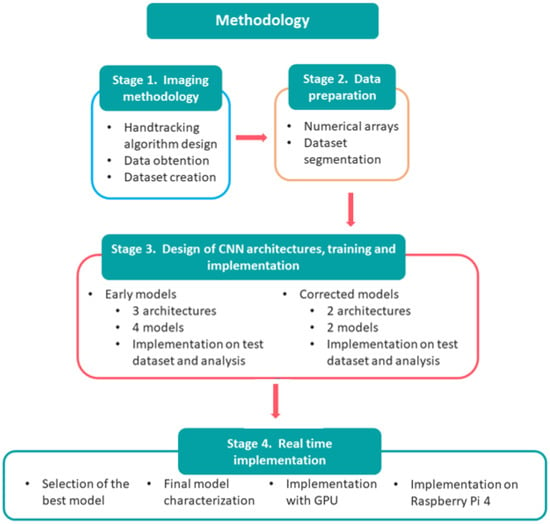
Figure 1.
Research methodology.
2.1. Stage 1. Imaging Methodology
The training data for the CNN models consisted of 3822 images, 182 for each of the 21 LSM hand alphabet static signs. All images were of the hands of a single individual. The following considerations were taken into account for the images:
- The signaling hand must be wholly contained within the image. MediaPipe is capable of inferring the positions of the wrist and all fingers, even when they are partially obscured or not fully visible, providing additional information that enhances the accuracy of hand landmark detection. With this, the minimum classification region was defined as the area that completely frames the hand, starting from the wrist towards the distal phalanges of all the fingers.
- The photographs must be in color, and their lighting must be such that it allows distinguishing the fingers and the hand’s position. In this way, it is favored that the model retains the position of the fingers as a characteristic to be taken into account and that it not only classifies based on the contour of the hand and the shapes of the region it delimits.
- The photograph must contain points and lines that outline the structure of the hand. The objective is to provide the algorithm with images that capture the entire gesturing hand, pose, and structural parts highlighted.
- The image must be equivalent to a photograph of a right hand. This statement is true if the hand used is the right hand or reflecting on an axis the capture of the signal when conducted with the left hand. This condition prevents the model from distinguishing between two cases of the same sign, reducing the number of images for training.
- The hand must cover the maximum possible region of the image without leaving this area. In other words, the hand should not look small relative to the photo and should be positioned in the center of the picture.
Figure 2 shows an example of a photograph of a hand sign that meets the considerations above.
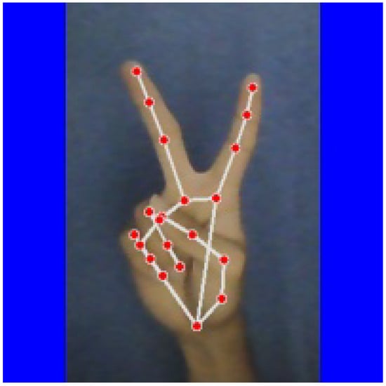
Figure 2.
An example of the image obtained for creating its own database is the Letter V of the dactylographic alphabet of LSM.
2.1.1. Hand Detection Algorithm
A hand detection algorithm based on MediaPipe and OpenCV functionalities was created to ensure the photographs met the above conditions. This algorithm extracted photographs that met the conditions described above from video frames from a webcam. Thanks to MediaPipe, this algorithm framed the area occupied by the hand in the image and identified its structural parts, which were schematized by points and lines drawn on the image. In addition, it had the task of identifying if the detected hand was right or left and reflecting it as required. The size of the photographs obtained was 200 × 200 pixels, one color and with a blue frame generated by the algorithm to reduce the presence of background elements in the final image. The set of images used in this study was formed only with photographs of the hands of an individual. Figure 3 shows examples of photographs obtained at this stage of all the letters.
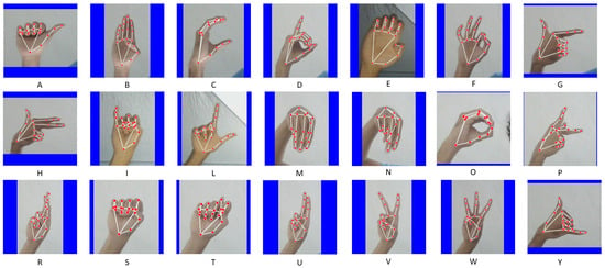
Figure 3.
Static signs of the finger alphabet with structural marks. Each image shows a static sign and below it is shown the letter it represents.
2.1.2. External Database
A similar database from a similar investigation was used ([17]) to verify if the considerations for the images positively impacted the final performance of models. These met all the considerations raised in this work except for the 1, 3, and 5:
- In some images, the wrist was not visible.
- Absence of structural marks.
- The hand’s position in the image is not centered, and there is no proportional relationship between the hand and the image.
This database was modified to the images containing the structural marks created by MediaPipe. However, the other two still needed to be fulfilled. With these data, a CNN model was compared with a similar one trained with our database. This external database is comprised of 4347 images of 200 × 200 pixels with three color channels; there are exactly 207 images for each of the 21 signs. In Figure 4, you can see an image of this base after being processed with MediaPipe.
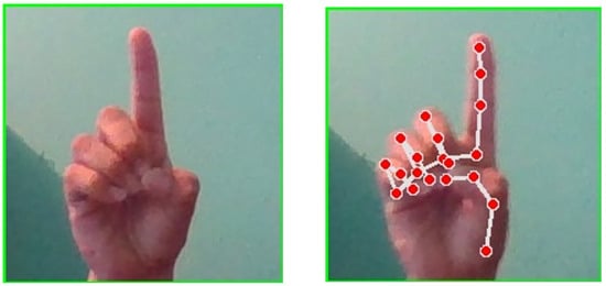
Figure 4.
Example of an image from an external database [17]. In this case, the wrist is not detected before and after processing the image with MediaPipe.
2.2. Stage 2. Data Preparation
The images were converted to numerical arrays to train CNN’s architectural proposals. In the case of our database, this resulted in a numerical arrangement of 3822 × 200 × 200 × 3 elements. For the external one, it was 4347 × 200 × 200 × 3 elements. In both, the first factor represents the total number of images, the following two the image size in pixels, and the latter is associated with RGB channels. A vector of labels useful for the learning process was created for each set. Each letter corresponds to a number, from 1 to 21, depending on its position in the alphabet.
No extra filters were applied since the goal was to minimize computational processing to favor the implementation in real time.
The initial data set was segmented into two samples: training and validation, the same ones used in the proposed architectures’ training process. The own and external databases were segmented into 80% for training and 20% for validation.
2.3. Stage 3. Design of Neural Network Architectures, Training, and Implementation of the Models
First, three architectures were proposed, from which four models were obtained. After analyzing them, two other architectures were proposed.
Features that were used for all architectures:
- ReLu activation function in all hidden layers
- softmax function for the output layer to have a probability vector as an output of the model
- Two-dimensional kernels of 3 × 3 and 5 × 5
- Pooling with Max Pooling function and 2 × 2 windows
- No padding
- 1 × 1 Stride
- Dropout ratio equal to 0.2
- Categorical Cross Entropy as a Loss Function
- Optimizer: ADAM
- Training with 40 epochs for the first models
- Training with 15 epochs for the second models
- Performance metrics: precision and loss
Early Models

Table 1.
The architecture of Network 1.

Table 2.
The architecture of Network 2.

Table 3.
The architecture of Network 3.
The proposed architectures are similar in the following:
- In their feature extraction stage, all of them implement at least two convolution stages, two pooling stages, and exactly one flattening stage where the data transitions from multidimensional arrays to linear arrays.
- The output layers have 21 neurons corresponding to each of the 21 signs.
The main differences between the architectures are as follows:
- Differences in dropout:
- –
- Architecture 1 does not implement dropout.
- –
- Architectures 1 and 2 are identical in every way except that Architecture 2 implements dropout, exactly twice, after the first two pooling stages.
- –
- Architecture 3 implements dropout in different layers than Architecture 2.
- Architecture 3 has a less deep feature extraction stage than Architectures 1 and 2, as it has one fewer convolution.
- Architecture 3 has an additional layer of neurons, and this layer is wider: it has three layers of neurons, while Architectures 1 and 2 have only two. This extra layer has 256 neurons, whereas in Architectures 1 and 2, the layer with the most neurons has 128.
A model was created with Architecture 1 based on external database images previously modified with MediaPipe. The training was carried out with data, and model 1 was generated. It was then compared with model 2, of the same architecture but trained with a different database, to verify if the considerations for the images had a positive impact on the performance of the final models.
The evaluation of the performance of the models with a sample other than the one used for their training was carried out with a set of images from 4 individuals (none of them participating in obtaining the training data). In total, 336 images were obtained, four for each letter for each individual, with the help of the detection algorithm and hand tracking. With the test results, the confusion matrices of each model for the test set were generated, and the models were concluded.
3. Results
This section presents the results of the proposed method and its comparison with other models.
3.1. First Models and Their Results
Table 4 summarizes the main characteristics of the first trained models, presenting values related to the training process and referring to the training and validation samples. The training and validation values of loss and accuracy presented in Table 4 correspond to those obtained in the last epoch of the training process.

Table 4.
Characteristics of the generated models.
Figure 5 depicts the learning curves of each of the models.
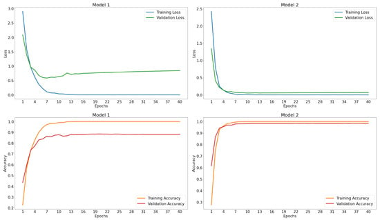
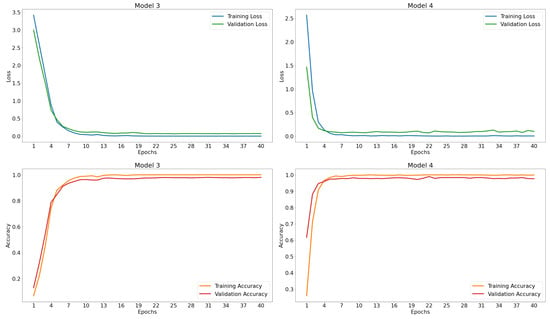
Figure 5.
Learning curves of the first four models.
3.2. Comparison between Model 1 and 2
The validation loss curve of Model 1 decreases to a minimum after epoch 5 and then tends to increase, slightly deviating from the training curve. This behavior indicates overfitting, as the loss in the training data remains stable within a specific range for the last epochs. However, the validation loss slightly increases, meaning that the model loses some of its generalization capability in the last epochs.
The comparison between Models 1 and 2 shows that the accuracy achieved by Model 1, 88.16%, on its validation set is considerably lower than that achieved by Model 2, which was 98.56%. The same behavior occurs with their losses on the validation set, with Model 1 having a higher loss than Model 2.
Since Model 1 and Model 2 have the same architecture but use different datasets for training and validation, the difference in their performance is attributed to the specific characteristics of the datasets used in their learning: the external dataset and the in-house dataset. These differences resulted from the data obtained and the considerations of the requirements that the images had to meet, aspects that were covered by the hand detection algorithm.
3.3. Models 2 to 3
Based on the information in Table 4 and the learning curves shown in Figure 5, the following observations can be made for models 2 to 3:
- There are no signs of underfitting.
- From the tenth epoch, both validation and training losses are below 0.5 and the accuracies are above 90%. In later epochs, there is some stabilization of the curves within a range of 90 to 100% for accuracy and 0 to 0.5 for loss.
- The final accuracy values for the training data are more significant than 99.00%, while those for the validation data are greater than 97.50%.
- The validation curves do not show a decreasing trend as the number of epochs increases.
- There are indications of overfitting. The training and validation curves, for both loss and accuracy, do not converge after the first intersection between them. This observation could be because:
- The models do not generalize well, but the training and validation data do not show significant differences, allowing for the stabilization of the curves.
- The models generalize well, but there are significant differences between the two datasets (validation and training).
The second cause is ruled out since the data belongs to the same sample and was obtained using the hand detection algorithm, which, after the comparison between models 1 and 2, showed a positive impact on the data collection process.
The first observation (1) indicates that the models adjusted correctly to the training data, so there is no evidence of underfitting. The last observation (2) does not rule out the presence of overfitting since it provides evidence of its presence.
To confirm the presence of overfitting, these models were tested on the test set. The results are shown in Table 5.

Table 5.
Performance of the models on test data.
Based on the observations made for the models regarding their performance obtained in the learning process and the results of this test, it was concluded that all models suffered from overfitting.
3.4. Results of the New Models
Two architectures were proposed to solve the overfitting with specific considerations:
- Decrease the number of epochs
- Reduce the capacity of the models
- Decrease the number of fully connected layers to 2
Increasing the number of training data was not considered due to time constraints, but all other considerations were applied to the new architectures. In each architecture, the capacity was reduced in two ways:
- Architecture 4The convolutional layers were reduced, and the number of neurons in the fully connected layer decreased; see Table 6.
 Table 6. The architecture of Network 4.
 - Architecture 5The depth of the model was increased by adding more convolutional layers. Additionally, the number of neurons was kept the same, but a dropout layer was added as a regularization process before the convolutional layers, as shown in Table 7.
 Table 7. The architecture of Network 5.
Table 8 summarizes the characteristics of the two models obtained with these architectures.

Table 8.
Characteristics of models 9 and 10.
Model 9 has more parameters than 2 and 3, its losses are higher than those of the previous models, and its accuracy achieved on the validation set is lower than in past models. On the other hand, model 10 has fewer parameters than all other models; its accuracy on the training data is within the range achieved by models 2 to 4, while its training loss is higher than the others. However, model 10 achieved better results on the validation data than models 2 to 4, as its validation loss was lower than theirs and its accuracy was higher.
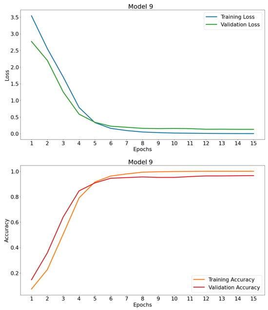
Figure 6.
Learning curves of model 9.
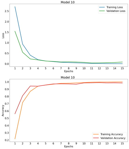
Figure 7.
Learning curves of model 10.
From the learning curves (Figure 6), it can be observed that Model 9 performs similarly to its predecessors. For Model 10, the curves (Figure 7) cut off at several points after stabilizing their values within the range of 90 to 100% accuracy after epoch 4; the same happens with the loss curves in the range of 0 to 0.5. This result indicates that the model generalizes its learning enough to correctly predict 98.43% on the validation set, appearing to have no overfitting. To confirm this observation, both models were implemented on the test set. Table 9 shows the performance of the models on this dataset.

Table 9.
Performance of Models 9 and 10 on Test Data.
Table 9 shows that model 10 performs better in predicting the test dataset than models 2 to 4 and 9, achieving lower loss and higher accuracy. On the other hand, the performance of model 9 is comparable to that of models 2 to 4, as its values are within the range achieved by the previous ones.
It is concluded that:
- Model 9 has overfitting.
- Model 10 does not have overfitting.
From the observations made on its training and the results of its test, it is confirmed that model 10 has the best performance in terms of its generalization ability.
3.5. Selection and Characterization of the Final Model
Since model 10 does not exhibit overfitting and achieved accuracy values of 99.93%, 98.43%, and 83.63% on the training, validation, and test datasets, respectively, it was chosen as the final model. Figure 8 shows the confusion matrix for the final model.
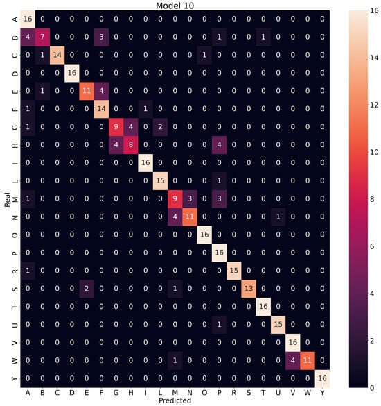
Figure 8.
Confusion matrix for model 10.
It is possible to calculate the following metrics that measure classification performance using the information from the confusion matrix:
- true positive (TP): is an outcome where the model correctly predicts the positive class.
- true negative (TN): is an outcome where the model correctly predicts the negative class.
- false positive (FP): is an outcome where the model incorrectly predicts the positive class.
- false negative (FN): is an outcome where the model incorrectly predicts the negative class
- precision or positive predictive value (PPV).
- sensitivity, recall, hit rate, or true positive rate (TPR)
- specificity, selectivity or true negative rate (TNR)

Table 10.
PPV, TPR and TNR, by letter, obtained by model 10.
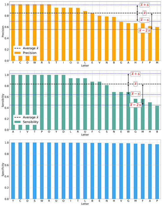
Figure 9.
Graphs of the precision, sensitivity, and specificity, by letter, obtained by model 10 on the test data.
- The letters N, B, G, A, H, F, P, and M have precision values lower than 0.8000, indicating that the final model was correct in classifying a sign as belonging to one of these classes less than 80.00% of the time. In the case of the letter M, its precision was 0.6000, meaning that of all the times a sign was classified as M, only 60.00% were correct.
- For two-thirds of the letters, the achieved sensitivity was higher than 0.8000. The remaining 7 letters were N, E, W, G, M, H, and B. The model correctly recognized and classified less than 80.00% of the examples for each letter.
- The obtained specificity values were higher than 0.9600, as can be seen in the corresponding graph, indicating that for each class, the model did not classify examples that did not belong to that class in more than 95.00% of the cases.
- The letters N, M, G, B, and H had precision and sensitivity values lower than 0.8000, making them the worst-classified letters by the model, as less than 80.00% of the classified examples in these letters actually belonged to them. The model detected less than 80.00% of the examples that actually belonged to these letters. For example, in the case of the letter H, only 66.67% of the classified examples were correct, and the model only detected half of the test set examples corresponding to that letter.
- The best-classified letters were D and Y, as their precision and sensitivity values were both equal to 1.000.
- The average of the values in the table, as reported in the same, keeps all values above 0.80.
3.6. Real-Time Implementation
The final system consisted of real-time implementation of the final model, the hand detection algorithm, and some OpenCV functionalities. Figure 10 shows the functioning of the final system and Figure 11 shows the system in operation.
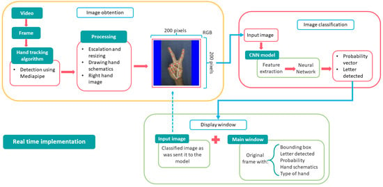
Figure 10.
Functioning scheme of the final system.
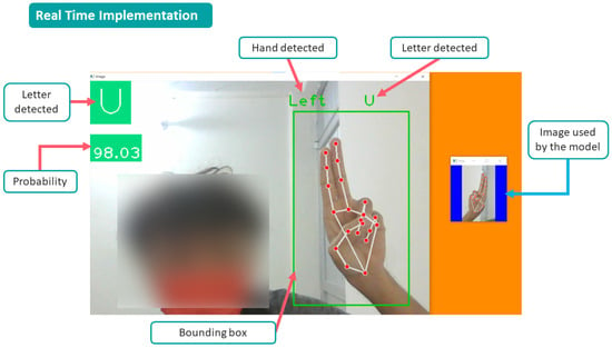
Figure 11.
Real-time testing.
The system was run on a computer with a GPU, and on one without a GPU; in both cases, the fluency of the operation was such that it can be considered that real-time classification of manual signs was achieved. The final system used functionalities from Keras for its execution on computers with a GPU. In the case of computers without a GPU, TFLite was used to run the model, eliminating the need for a GPU and thus guaranteeing the accessibility of the final system implementation. As a result, it was possible to implement it on a computer with a GPU as well as on a Raspberry Pi 4 - 2G (see Figure 12) using TFLite, in this case, the delay between the gestured sign and the one displayed on the screen was noticeable, with an average delay of 0.58s obtained after testing.
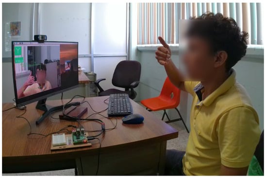
Figure 12.
Implementation of the final system on the Raspberry Pi 4, with an average response time of 0.58 s.
3.7. Technical Limitations and Improvement Proposals
Based on the technical limitations observed during the real-time testing, some proposals for improvement are as follows:
- The input images to the models must comply with the specifications outlined previously.
- The machine learning model’s performance depends on the hand detection and tracking algorithm to obtain and process images. If this algorithm fails, then the classification is defective.
- The lighting on the hand and the color of the image background. The hand detection algorithm fails when the background color resembles the color of the hand or when the hand is not visible. In these cases, the hand’s position that is schematized with lines and points may not correspond to the real position of the hand.
- Sign classification depends on the view from which they are shown to the camera. The origin of this limitation arises from the training dataset, whose views for each sign are limited. By views, we mean lateral, frontal, superior, and posterior. For the views used in the training process, certain variations in their perspective were considered, but not enough to be considered as a different view. An example of this occurs with the letter D; a lateral view was used for its training, and the model predicts another letter when a frontal view is used. In Figure 13, it can be seen how the letter D is confused with the letter I when changing the view.
 Figure 13. Confusion between the letters D and I due to the difference in appearance.
 - The letters worst classified by the final model were N, M, B, G, and H because they had values less than 0.80 in precision and sensitivity (see Table 10). From the confusion matrix of model 10 (see Figure 8), it is highlighted that the letters G and H were confused with one another. This situation is attributed to the multiple convolution stages, which condensed the characteristics of the index and middle fingers, making it difficult for the model to distinguish between the case where only the index finger was extended and the case when the middle finger accompanied it. Something similar happened with the letters W and V. It is important to highlight that the letters’ precision, sensitivity, and specificity estimates were obtained with the test dataset, which was limited to only four individuals. Expanding the test dataset to consider hands into a broader spectrum of physical complexions is necessary to obtain more representative population values. As the test dataset is expanded, the degree of generalization achieved by the final model over the population in general can be determined more accurately.
- Even when the input image to the classifier model is a hand that does not represent any sign in the finger alphabet, the model will classify it within one of the 21 classes associated with the letters. An example of this is presented in Figure 14.
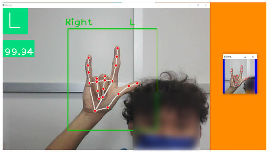 Figure 14. Classification of a sign that does not belong to the finger alphabet.
 - To address the dependence on the distance between the hand and the camera. The structural points of the hand that are drawn on it are not scaled to maintain a proportion with respect to the pixel size of the area on which the hand is framed, causing the schematic points to overlap at specific distances between the hand and the camera, hindering the classification task of the models. For example, in Figure 15, the sign of the letter C is classified as O when the hand moves away from the camera. This condition is not a significant problem, as it can be solved by modifying MediaPipe to maintain proportionality between points and the captured hand.
 Figure 15. Confusion between the letter C and O due to the distance.
4. Discussion
Similar works have focused on American Sign Language (ASL) signs, which present similarities to those of Mexican Sign Language (LSM) covered here. The 21 static signs of the LSM manual alphabet have slight differences from their counterparts in ASL; in addition, the latter has static signs for the letters K, Q, and X. These investigations use various methodologies, two of which are highlighted for their similarity to this work:
- Methodologies are based on classifying and recognizing images of hands gesturing a sign. The images are sent to AI models trained for recognition and classification.
- Methodologies are based on the classification of 2D spatial coordinate values associated with structural points of the hands. Currently, Mediapipe predominates for these, as it allows the generating coordinates of structural points of the hands, which AI models process for their classification and interpretation.
Regarding the methodology of this research, the following is highlighted:
- Classification based on enriched images.
- Use Mediapipe to enrich hand images by tracing points and lines that schematize the hand’s structure.
- Use of convolutional neural networks for the classification process of photographs.
Regarding the classification of coordinates, it is noteworthy that Masanao Yasumuro and Kenya Jin’no’s research [19] achieved 100% accuracy on their validation set. In that project, the 24 static letters of ASL were covered, and more than 1200 example samples were obtained for each one, segmented into 80% for training and 20% for validation. The classification was conducted with a LinearSVM and used 2D data of hand point coordinates obtained with MediaPipe. From Table 8, it can be seen that the accuracy of model 10 in this project was 98.43%, using six times fewer training examples for each sign. The work of Sundar B, Bagyammal T [20] achieved 99% accuracy on a validation set in the recognition of 36 ASL signs, using MediaPipe and LSTM. On the other hand, Arpita Haldera and Akshit Tayade [11] achieved 99.15% accuracy using an SVM, 98.21% with a KNN, 98.57% with a random forest and a decision tree, 97.12% with an ANN, and 94.69% using an MLP. The accuracy achieved here (98.43%) with a CNN is within the range obtained in all previous investigations. Unlike this work, the previous methodologies were oriented towards classifying the coordinates of the 21 points generated by MediaPipe when detecting a hand; it is worth noting.
Regarding image classification, Prangon Das, Tanvir Ahmed, and Md. Firoj Ali [21] developed a methodology for recognizing static ASL signs using Deep CNN, achieving a validation accuracy of 94.34%. This accuracy value was higher than several existing examples up until that year that employed methodologies based on the use of Kinect or an AlexNet configuration ([22]). MediaPipe was not used in this study, and fewer training data were employed in the current research than those used for Model 10.
Murat Taskiran, Mehmet Killioglu, and Nihan Kahraman [23] achieved an accuracy of 98.05% using a CNN operated in real time. The classification system required determining skin color and the shape and location within the frame. These last two steps were achieved using the convex hull algorithm, which generated images sent to the model for classification. This detection-classification hand methodology is similar to the one addressed in this study, except that MediaPipe was used to handle hand color, detection, and location. Nevertheless, the accuracy value results are similar. Therefore, MediaPipe allowed for the elimination of certain pre-processing stages.
After comparing the performance of models 1 and 2 regarding the hand detection algorithm, it was observed that both models had overfitting, but it was more pronounced in model 1. The images generated by the hand-tracking algorithm helped prevent overfitting. The generated images allowed for a lower error and higher accuracy in the validation data. This observation is attributed to the fact that the algorithm ensured that the generated images correctly framed the hand without losing any of its areas of interest and maintained a relationship between the image and the captured hand. As a result, the CNN did not need to learn to identify manual alphabet signs whose presence in images needs to include specific data, such as a missing finger or wrist location. In this way, the algorithm reduced the workload of the neural network, which contributed to requiring less complexity to fit the training data. Equivalently, it reduced the amount of training information required for the trained models to achieve a certain level of performance in their tests.
Architectures 1, 2, 3, and 4 had more capacity than required for the problem, which resulted in overfitting for the models generated from these architectures: 2, 3, 4, and 9, respectively. The CNN architecture best adapted to the sign classification was architecture 5, which had more convolution and pooling stages, fewer hidden layers, applied dropout for regularization, and fewer parameters (see Table 7). The best-performing model in the tests was obtained with architecture 5, and overfitting was avoided. The architecture alone was not solely responsible for its performance in the tests; the hand detection algorithm also had an influence. Model 10 was selected as the final model due to its good performance.
The final CNN model accomplished an accuracy of 83.63% on the test set, which was achieved due to the absence of signs of underfitting and overfitting in the final model, indicating good generalization capacity. This behavior corresponds to the fact that the capacity of the final model is suitable for the training sample. However, the model’s generalization was also conditioned by how representative various users concerning the population, which in this case consists of manual signs of the dactylological alphabet of LSM gesture the training sample with a great variety of differences in the shape and size of their hands and components.
Within the context above, the final system of this research presents an alternative methodology to existing ones. It achieves similar results in classifying static signs of a manual alphabet, in this case, the LSM. The advantages of this methodology over existing ones are the use of a smaller amount of training data, the absence of image pre-processing stages based on filters, and the use of small CNN architectures. These advantages were made possible using MediaPipe, allowing for real-time implementation.
5. Conclusions
When applied to images and video frames, the hand detection algorithm accomplished its task. It obtained images containing graphical information about the hand structure drawn on it and other considerations related to the type of hand and the proportionality between the hand and the image. The proper functioning of this algorithm was influenced by the lighting conditions of the environment and background, with this influence accentuating when the background color was similar to the skin color of the hand.
The training set was composed solely of photographs of one person; however, the hand detection algorithm was used to abstract the characteristics of the photographed hand through its schematic representation with points and lines to reduce the dependence of the trained models on data such as skin color, specific finger shapes, and finger size. The final model achieved a level of precision in the test data of 83.63%, which corresponded to a different type of hands. Therefore, it can be said that enriching the images with schematic drawings proved to be beneficial for the performance of the models, as this provided them with extra information about the hand’s position, which is more abstract than just having the image of the hand itself. As a result, the final model can generalize with a reasonable degree of precision on a test data set different from its training data. This result is noteworthy, given that only 166 images per letter were used for training, and these were taken from the hands of only one individual. Increasing the number of training samples and making them more diverse is recommended to increase their representativeness.
Since real-time classification consisted of implementing the final model together with the hand detection algorithm, its operation was conditioned to the operation of both. The fluency in implementing the final system was achieved by avoiding previous filters on the input images and keeping the final CNN model with few parameters (363, 365), compared to the other models obtained in this study. With this, it was possible to make the implementation computationally accessible for devices with limited resources, such as a Raspberry Pi 4 or laptops without a GPU and few processing cores.
The average, per letter, of precision, sensitivity, and specificity obtained by the final model were, respectively, 84.57% with a standard deviation of 14.55%, 83.33% with a standard deviation of 19.20%, and 99.17% with a standard deviation of 0.92%. The letters best classified by the final model were D and Y, with a precision and sensitivity of 100% during testing. The worst classified letters were N, M, B, G, and H. In the case of the last letters, the model confused them. It is believed that due to multiple convolutions, the model found it challenging to distinguish between the case when only the index finger was extended and the case when the middle finger accompanied it, as convolutions contributed to mixing and condensing the features of these fingers, negatively impacting the classification. Something similar happened with the letters W and V.
This project can serve as a didactic tool aimed at introducing and training new users of sign language, which is efficient in its work and, above all, accessible for its implementation, meaning that it requires few computational and economic resources, thus presenting itself as a viable solution for implementation.
Author Contributions
Conceptualization, T.J.S.-V., A.A.C.-A., E.C.-P., M.C.-F. and E.C.-P.; Methodology, E.C.-P., M.C.-F., A.A.C.-A. and J.R.-R.; Writing original draft preparation, T.J.S.-V., M.C.-F., J.R.-R. and E.C.-P.; Writing, review and editing, A.A.C.-A., J.R.G.-M. and T.J.S.-V.; Supervision, E.C.-P., T.J.S.-V., J.R.G.-M. and M.C.-F. All authors have read and agreed to the published version of the manuscript.
Funding
This research received no external funding.
Institutional Review Board Statement
Not applicable.
Informed Consent Statement
Not applicable.
Data Availability Statement
Data will be made available on request.
Conflicts of Interest
The authors declare that they have no known competing financial interests or personal relationships that could have appeared to influence the work reported in this paper.
References
- Cheok, M.J.; Omar, Z.; Jaward, M.H. A review of hand gesture and sign language recognition techniques. Int. J. Mach. Learn. Cybern. 2019, 10, 131–153. [Google Scholar] [CrossRef]
- Abernathy, E.R. An historical sketch of the manual alphabets. Am. Ann. Deaf. 1959, 104, 232–240. [Google Scholar]
- Carmona-Arroyo, G.; Rios-Figueroa, H.V.; Avendaño-Garrido, M.L. Mexican Sign-Language Static-Alphabet Recognition Using 3D Affine Invariants. In Machine Vision Inspection Systems, Volume 2: Machine Learning-Based Approaches; Scrivener Publishing LLC: Beverly, MA, USA, 2021; pp. 171–192. [Google Scholar]
- Rautaray, S.S.; Agrawal, A. Vision based hand gesture recognition for human computer interaction: A survey. Artif. Intell. Rev. 2015, 43, 1–54. [Google Scholar] [CrossRef]
- Zhou, Z.; Chen, K.; Li, X.; Zhang, S.; Wu, Y.; Zhou, Y.; Meng, K.; Sun, C.; He, Q.; Fan, W.; et al. Sign-to-speech translation using machine-learning-assisted stretchable sensor arrays. Nat. Electron. 2020, 3, 571–578. [Google Scholar] [CrossRef]
- Alsaadi, Z.; Alshamani, E.; Alrehaili, M.; Alrashdi, A.A.D.; Albelwi, S.; Elfaki, A.O. A real time Arabic sign language alphabets (ArSLA) recognition model using deep learning architecture. Computers 2022, 11, 78. [Google Scholar] [CrossRef]
- Neto, G.M.R.; Junior, G.B.; de Almeida, J.D.S.; de Paiva, A.C. Sign language recognition based on 3d convolutional neural networks. In Proceedings of the Image Analysis and Recognition: 15th International Conference, ICIAR 2018, Póvoa de Varzim, Portugal, 27–29 June 2018; Proceedings 15. Springer: Berlin/Heidelberg, Germany, 2018; pp. 399–407. [Google Scholar]
- Bantupalli, K.; Xie, Y. American sign language recognition using deep learning and computer vision. In Proceedings of the 2018 IEEE International Conference on Big Data (Big Data), Seattle, WA, USA, 10–13 December 2018; pp. 4896–4899. [Google Scholar]
- Elhagry, A.; Elrayes, R.G. Egyptian sign language recognition using CNN and LSTM. arXiv 2021, arXiv:2107.13647. [Google Scholar]
- Gao, Y.; Jia, C.; Chen, H.; Jiang, X. Chinese fingerspelling sign language recognition using a nine-layer convolutional neural network. EAI Endorsed Trans. e-Learn. 2020, 7, e2. [Google Scholar] [CrossRef]
- Halder, A.; Tayade, A. Real-time vernacular sign language recognition using mediapipe and machine learning. Int. J. Res. Publ. Rev. 2021, 2, 9–17. [Google Scholar]
- Morfín-Chávez, R.F.; Gortarez-Pelayo, J.J.; Lopez-Nava, I.H. Fingerspelling Recognition in Mexican Sign Language (LSM) Using Machine Learning. In Proceedings of the Mexican International Conference on Artificial Intelligence, Yucatán, Mexico, 13–18 November 2023; Springer: Berlin/Heidelberg, Germany, 2023; pp. 110–120. [Google Scholar]
- Bora, J.; Dehingia, S.; Boruah, A.; Chetia, A.A.; Gogoi, D. Real-time assamese sign language recognition using mediapipe and deep learning. Procedia Comput. Sci. 2023, 218, 1384–1393. [Google Scholar] [CrossRef]
- Duy Khuat, B.; Thai Phung, D.; Thi Thu Pham, H.; Ngoc Bui, A.; Tung Ngo, S. Vietnamese sign language detection using Mediapipe. In Proceedings of the 2021 10th International Conference on Software and Computer Applications, Kuala Lumpur, Malaysia, 23–26 February 2021; pp. 162–165. [Google Scholar]
- Wang, Y.; Li, R.; Li, G. Sign language recognition using Mediapipe. In Proceedings of the International Conference on Computer Graphics, Artificial Intelligence, and Data Processing (ICCAID 2022), Guangzhou, China, 23–25 December 2022; SPIE: Bellingham, WA, USA, 2023; Volume 12604, pp. 807–813. [Google Scholar]
- Saiful, M.N.; Al Isam, A.; Moon, H.A.; Jaman, R.T.; Das, M.; Alam, M.R.; Rahman, A. Real-time sign language detection using cnn. In Proceedings of the 2022 International Conference on Data Analytics for Business and Industry (ICDABI), Sakhir, Bahrain, 25–26 October 2022; pp. 697–701. [Google Scholar]
- Morales, E.M.; Aparicio, O.V.; Arguijo, P.; Armenta, R.Á.M.; López, A.H.V. Traducción del lenguaje de señas usando visión por computadora. Res. Comput. Sci. 2019, 148, 79–89. [Google Scholar] [CrossRef]
- Lugaresi, C.; Tang, J.; Nash, H.; McClanahan, C.; Uboweja, E.; Hays, M.; Zhang, F.; Chang, C.L.; Yong, M.; Lee, J.; et al. MediaPipe: A Framework for Perceiving and Processing Reality. In Proceedings of the Third Workshop on Computer Vision for AR/VR at IEEE Computer Vision and Pattern Recognition (CVPR) 2019, Long Beach, CA, USA, 17 June 2019. [Google Scholar]
- Yasumuro, M.; Jin’no, K. Japanese fingerspelling identification by using MediaPipe. Nonlinear Theory Its Appl. IEICE 2022, 13, 288–293. [Google Scholar] [CrossRef]
- Sundar, B.; Bagyammal, T. American Sign Language Recognition for Alphabets Using MediaPipe and LSTM. Procedia Comput. Sci. 2022, 215, 642–651. [Google Scholar] [CrossRef]
- Das, P.; Ahmed, T.; Ali, M.F. Static hand gesture recognition for American sign language using deep convolutional neural network. In Proceedings of the 2020 IEEE Region 10 Symposium (TENSYMP), Dhaka, Bangladesh, 5–7 June 2020; pp. 1762–1765. [Google Scholar]
- Krizhevsky, A.; Sutskever, I.; Hinton, G.E. Imagenet classification with deep convolutional neural networks. Commun. ACM 2017, 60, 84–90. [Google Scholar] [CrossRef]
- Taskiran, M.; Killioglu, M.; Kahraman, N. A real-time system for recognition of American sign language by using deep learning. In Proceedings of the 2018 41st International Conference on Telecommunications and Signal Processing (TSP), Athens, Greece, 4–6 July 2018; pp. 1–5. [Google Scholar]
Disclaimer/Publisher’s Note: The statements, opinions and data contained in all publications are solely those of the individual author(s) and contributor(s) and not of MDPI and/or the editor(s). MDPI and/or the editor(s) disclaim responsibility for any injury to people or property resulting from any ideas, methods, instructions or products referred to in the content. |
© 2024 by the authors. Licensee MDPI, Basel, Switzerland. This article is an open access article distributed under the terms and conditions of the Creative Commons Attribution (CC BY) license (https://creativecommons.org/licenses/by/4.0/).