1. Introduction
Artificial intelligence (AI) and machine learning (ML) have dramatically improved human life by bringing a revolution in many areas [
1]. AI-powered systems are integrated into everyday activities, from the technology embedded in smartphones to the personalized recommendations in online shopping. Although AI has brought many changes to the world, we need to develop robust safety ML algorithms to get the benefits of technology [
2]. The algorithms trained with safety model can be utilized to monitor and guide online actions for safety compliance [
3]. Creating an AI safety culture is essential in all workflows of ML development, from data gathering to product deployment. Reinforcement Learning (RL) is an important area of ML where an agent interacts with an unknown environment and tries to act in an optimal way by learning the dynamics of that environment [
4]. Therefore, the safety aspect of learning about RL agents is more important.
RL, being a useful AI technology, is used in diverse domains [
5]. RL algorithms have significant application in many areas including healthcare [
6], UAVs, 5G and autonomous control [
7], gesture classification [
8], risk management [
9], communication [
10], and clinical assistance [
11,
12]. The increasing use of RL in many areas is a reflection of its exceptional ability to address complex problems that are sometime intractable for conventional ML techniques. However, the universal suitability of RL calls for a multi-faceted research mechanism, confining real-world validations, safety measures, and algorithmic improvements [
13]. Researchers need to address questions like: are rewards on their own enough for the optimality of an RL model?
Although rewards are the basic metric in RL setup, an overemphasis on accumulated rewards may result in a misleading solution or evaluation. Therefore, this research work focuses on the definition of new metrics to manage hazardous situations or states alongside optimizing rewards.
This field is characterized by numerous challenges, including uncertainties or considerable delays in system sensors, actuators, or rewards; the necessity for real-time inference at the system’s control frequency; the demand for actions and policies that are explainable by system operators; reward functions that are sensitive to risks, multi-objective, or unspecified; tasks that are non-stationary or stochastic; high-dimensional continuous action and state spaces; learning on real systems with limited samples; and offline training from fixed logs of an external behavior policy.
The two metrics proposed in this study address several critical aspects of the challenges. Firstly, the Hazard Indicator provides a measure of the overall hazard associated with each state, enabling the agent to recognize and avoid states with high probabilities of leading to failure. This addresses the challenge of integrating safety considerations into the learning process and ensures that the agent does not solely focus on maximizing rewards at the expense of safety. The Risk Indicator, on the other hand, quantifies the level of risk by incorporating the cost implications of potential failure states. This helps manage risk-sensitive, multi-objective reward functions and ensures that the agent accounts for the severity of different failure states. By balancing risk and reward, the agent can make more informed decisions, thereby enhancing the safety and reliability of RL in practical applications.
By leveraging these metrics, RL agents can substantially enhance the realization and implementation of RL in practical applications, bolstering their reliability and efficacy
The rest of the paper is organized as follows:
Section 2 provides an essential overview of RL and the safety aspects associated with it, addressed to readers who may encounter the concept for the first time;
Section 3 briefly overviews the related work.
Section 4 and
Section 5 present the proposed definitions and experiments, respectively. In
Section 6, an application of the metric to a real scenario is given. In the last section, we draw some conclusions.
2. Technical Background
Reinforcement Learning (RL) is a computational learning approach that deals with learning in sequential decision-making problems conditioned by feedback as demonstrated in the
Figure 1. It is one of three main machine learning paradigms, with supervised learning (which needs labeled input/output pairs to infer a mapping between them) and unsupervised learning (which analyzes a large quantity of unlabeled data to capture patterns from them).
RL algorithms are characterized by four basic elements: an agent, a program to train for a certain purpose; the environment, the world in which the agent can stay and performs actions, in practice, a collection of state signals; an action, a movement made by the agent that allows to switch from one state to another in the environment; and a reward signal (or simply reward), the evaluation of an action, a numerical feedback from the environment. The agent must discover which actions yield the most reward by trying them: the data are generated with a trial-and-error search during training within the environment and marked with a label. The mapping from states to actions (to be taken when in those states) is called a policy. The policy can be described as one mathematical function, a lookup table, or a more complex computational process (e.g., a neural net whose input is a representation of the state and its output an action selection probability). In other words, solving an RL task means finding a policy called optimal policy that maximizes the total reward signal over time.
Typically, an RL problem is mathematically formulated through the Markov Decision Process framework; this can be represented by a tuple , where
S is the set of all possible states.
A is the set of all possible actions.
P is the state transition probability function, , which represents the probability of transitioning to state from state by taking action .
R is the reward function, also called cost function, , which provides the immediate reward received after transitioning from state to state due to action .
is the discount factor, , which represents the importance of future rewards.
The policy defines the probability of taking action when in state .
The goal of the agent is to learn a policy
that maximize the expected discounted cumulative reward (i.e., the sum of all rewards received, scaled by a certain discount factor); in mathematical notation,
where
represents the reward obtained at time step
. The initial time step is referred to as
. The terminal step, denoted by
T, can be either a finite time horizon or infinity.
Generally, to quantify the worth of a state, value functions and an action–value function are used. The value function
represents the expected return starting from state
s, under policy
:
where
is the return starting from time step
t, and
denotes the expected value under policy
. The action–value function, the Q-function
, represents the expected return starting from state
s, taking action
a, and then following policy
:
This type of learning allows one to automate the resolution of complex control and interaction problems with the environment, in many cases not solvable with explicitly programming, potentially proposing the best possible solution.
RL, while effective in complex applications, is not inherently suited for safety-critical contexts due to challenges in ensuring policy safety and exploring unfamiliar states. Exploratory strategies often rely on occasional random actions, risking unsafe outcomes. Consequently, RL in real-world safety-critical systems is typically limited to simulation software. To address this, safe RL methods have emerged. Safe RL aims to minimize the potential for harmful actions during the learning process within RL frameworks (i.e., during the process of learning policies that maximize the expectation of the return). This is especially important in real-world applications like robotics, autonomous driving, and healthcare, where unsafe actions can have serious consequences. Currently these methods can be broadly categorized into two approaches: safe optimization (also referred to as modification of the optimality criterion) and safe exploration (otherwise known as modification of the exploration process) [
14].
Safe optimization integrates safety considerations into the policy, often via constraints ensuring policy parameters remain within a defined safe space. These algorithms can incorporate a risk measure of encountering unsafe situations, depending on the specific tasks. Safe exploration aims to prevent the selection of unsafe actions during training, leveraging external knowledge to guide exploration.
3. Related Work
This section briefly reviews a few research works that consider any aspect of safe reinforcement learning. A fundamental concept was given in [
15], where authors introduced the idea of a probabilistic shield to improve the safety of RL algorithms. They utilized formal verification methods to calculate the probabilities of critical decisions within a safety-related fragment of Markov Decision Processes (MDPs). This work demonstrated enhanced learning efficiency in several scenarios such as service robots and the arcade game PAC-MAN. On the other hand, the authors of [
16] considered the synergy between RL and model checking for scalable mission planning including many autonomous agents. Although that work was useful for complex mission planning problems, an experimental validation was missing.
A safe deep RL approach was developed in [
2] in a networked microgrid system for the hierarchical coordination between individual microgrids towards decentralized operation. In the first stage of this two-stage methodology, energy storage systems and active power outputs of micro-turbines were scheduled on an hourly basis for cost minimization and energy balancing, while in the second stage, the reactive power outputs of PV inverters were dispatched every three minutes based on a Q/V droop controller to regulate voltage and to minimize network power losses under real-time uncertainties. A similar work was conducted in [
17] where the authors proposed a two-stage multi-agent deep RL scheme for the reconfiguration of an urban distribution network by presenting a switch contribution concept. The authors in [
18] introduced a federated learning method to integrate a transformer model and proximal algorithm for vehicle-to-grid scheduling. The authors used an end-to-end deep learning framework using current and historical data to decide scheduling under uncertainties.
Model-Agnostic Meta-Learning is employed in [
19] by considering learning about tasks within a distribution, and it can adapt quickly to solve a new unseen in-distribution task. A bootstrap deep Q-network is used in [
20] to learn an ensemble of Q-networks. The model also utilizes Thompson’s sampling to drive exploration and enhance sample efficiency. The use of expert demonstrations to bootstrap the agent can improve sample efficiency. This methodology is applied in [
21] by combining it with a deep Q-network. This method is also demonstrated on Atari games in [
22]. A real system does not have a separate environment for training and evaluation, which is unlike most of the research conducted in deep RL [
22]. The data for training come from the real system where an agent cannot have a separate exploration policy during training, as its exploratory actions do not come for free. In fact, an agent’s performance must be reasonably good and should act safely throughout learning. This means that exploration must be limited for many systems and consequently, the resulting data have low variance—very little of the state space may be covered in the logs. Moreover, there is often only one instance of the system; schemes that instantiate hundreds or thousands of environments to collect more data for distributed training are normally not compatible with this setup [
23,
24]. In [
25], the authors consider mobile agent path planning in uncertain environments by integrating a probabilistic model with RL.
This work proposes the Hazard Indicator and Risk Indicator as novel metrics to assess the safety of an environment. These metrics leverage the concept of transition probabilities to failure states over a specified time horizon. The Hazard Indicator provides a general measure of the likelihood of encountering any failure state from a given state, while the Risk Indicator incorporates the potential cost associated with each failure state.
The development of robust metrics for evaluating safety in RL environments is crucial for the successful deployment of RL algorithms in real-world applications.
4. Defining the Metrics
This section formally defines the metrics used to evaluate the safety of an environment with respect to failure states. We begin by defining the Markovian state space, comprising both safe and failure states, and then introduce probabilistic measures capturing the likelihood of transitioning between these states over a specified time horizon. Leveraging these probabilistic formulations, we introduce two indicators: the Hazard Indicator and the Risk Indicator. These indicators afford insights into the degree of hazard and risk associated with individual states within the system, thereby facilitating informed decision-making and risk mitigation strategies.
Safe states represent configurations within the environment where an agent’s actions, or simply its presence, do not lead to any negative and undesirable consequences. These states are considered non-critical because the agent can execute automated strategies and methods without any risk.
Failure states, conversely, are configurations within the environment that pose a significant threat to the agent’s structural integrity or the surrounding environment. If the agent enters a failure state, its execution of automated strategies and methods may cause damage to itself or its environment.
State space: we assume there are N possible discrete states within the environment, , K being safe states, M failure states, and .
Definition 1 (Transition Probability to Failure State).
The factor represents the total probability starting from state , at time t, to reach the specific failure state , after executing at maximum of l steps: In the base case, when
, we have:
Definition 2 (Hazard Indicator).
The Hazard Indicator, denoted by , represents the overall degree of hazard associated with that state : This indicator is particularly informative when all failure states M carry equal cost. If this assumption does not hold, it becomes crucial to consider the associated costs. Let us assume are the costs associated with the M failure states, respectively.
Definition 3 (Risk Indicator).
The Risk Indicator, denoted by , quantifies the level of risk associated with the state , by integrating the cost implications associated with individual potential failure states: Note: It is essential to acknowledge that the value of the parameter l is contextually dependent. However, the experimental phase revealed that excessively large values of l could compromise the effectiveness of the indicator. Accordingly, it is advisable to select values of l that enable us to operate in close proximity to failure states. This optimization ensures the metric’s practical usefulness.
5. Experiments
In the experimental phase, we considered the interaction of an agent within a simulation environment modeled as a stationary Markov Decision Process (MDP). This study employed a mobile robot model navigating a spatial environment discretized into states represented by a grid structure. Various scenario configurations were utilized to evaluate the efficacy and adaptability of the aforementioned Hazard and Risk Indicators.
Case 1 The agent navigates a grid with a single failing terminal state. All possible actions sampled by the agent are equiprobable, meaning each action has a 25% chance of being selected.
Case 2 Similar to Case 1, all actions are equiprobable; however, in this case, the grid contains two failing terminal states with identical associated costs.
Case 3 The grid structure remains the same as Case 2, featuring two failing terminal states. However, the costs associated with reaching each terminal state differ.
Case 4 The grid configuration reverts to a single failing terminal state. However, we introduced some systemic disturbing factors: for each step, the agent has a 70% probability of moving up. There is also a 10% chance of transitioning to any of the other three directions (down, left, or right).
5.1. Design of Experiments
The overarching goal of these experiments was to evaluate the effectiveness of the Hazard Indicator and Risk Indicator within domains that can be effectively represented using a Markovian framework. To achieve this, a two-dimensional grid-world environment was constructed. This world consisted of a 10 × 6 grid, yielding a total of 60 accessible states. Depending on the experimental condition, one or two of these states were designated as failure states, while the remaining states were considered safe. The agent’s action space was comprised of four discrete actions: up, down, right, and left. In each experiment, the following conditions held:
Limited exploration steps: the agent was restricted to a maximum of three actions, or more precisely three state transitions, i.e., .
Boundary handling: upward movements directed towards the grid’s edges resulted in the agent’s position remaining unchanged.
Early termination upon failure encounter: if the agent encountered a failure state during the first step, exploration was immediately terminated.
5.2. Experiment: Case 1
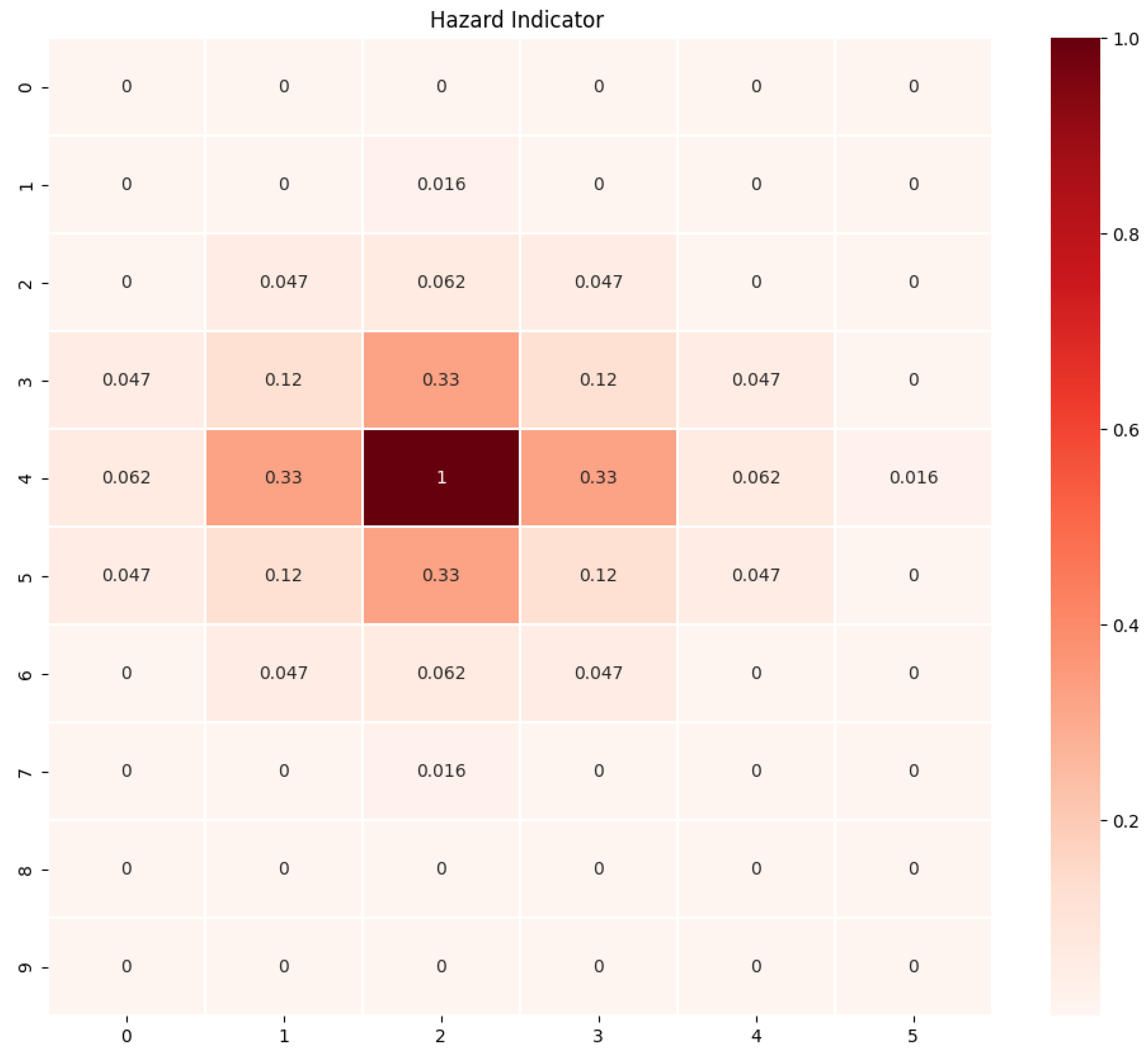
To promote a comprehensive understanding of the proposed approach, we commenced our investigation with a well-defined scenario. Within this scenario, only one of the 60 accessible states was designated as a failure state. Furthermore, the probability distribution governing the agent’s actions was uniform across all states. In simpler terms, each action (up, down, left, right) had an equiprobable chance of being selected. In the heatmap shown in
Figure 2, the Hazard Indicator values obtained,
, are displayed. These values represent the hazard level associated with each state.
To illustrate the results, consider the state located at row 5 and column 2. From this state, there exist six paths with a maximum of three steps that lead to the failure state. These paths are enumerated as follows: [’right’, ’left’, ’up’], [’right’, ’up’, ’left’], [’left’, ’right’, ’up’], [’left’, ’up’, ’right’], [’up’], and [’down’, ’up’, ’up’]. The total probability of reaching the failure state from this starting state can be calculated as follows: (0.016 × 5) + (0.25). The first term represents the sum of probabilities for the five paths (excluding [’up’]). Each of these paths has a probability approximately equal to 0.016 (obtained by multiplying the individual action probabilities: 0.25 × 0.25 × 0.25). The second term (0.25) represents the probability of reaching the failure state directly in a single step: ’up’.
5.3. Experiment: Case 2
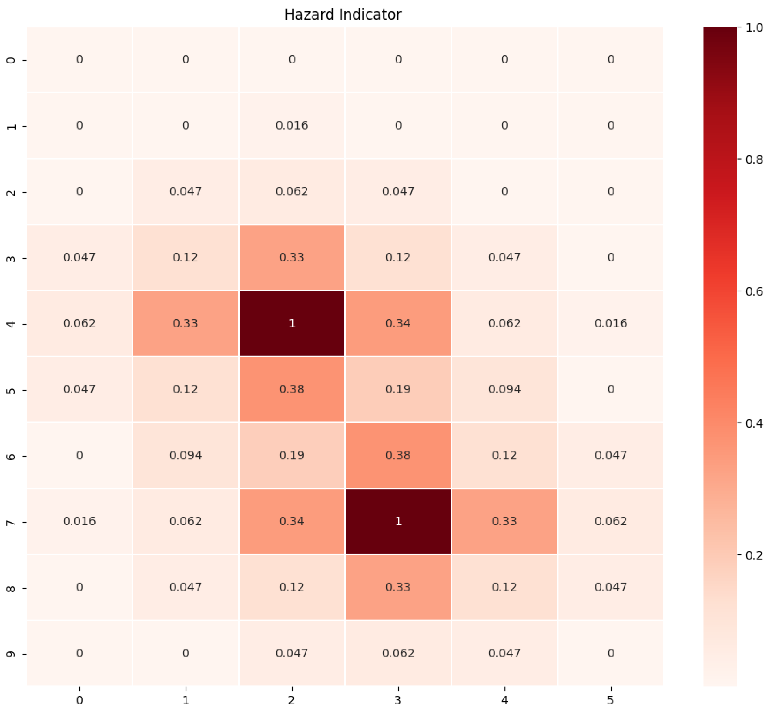
To introduce a level of complexity, we opted to work with two failure states. These failure states were assigned equivalent costs. The heatmap in
Figure 3 presents the obtained results from this scenario.
5.4. Experiment: Case 3
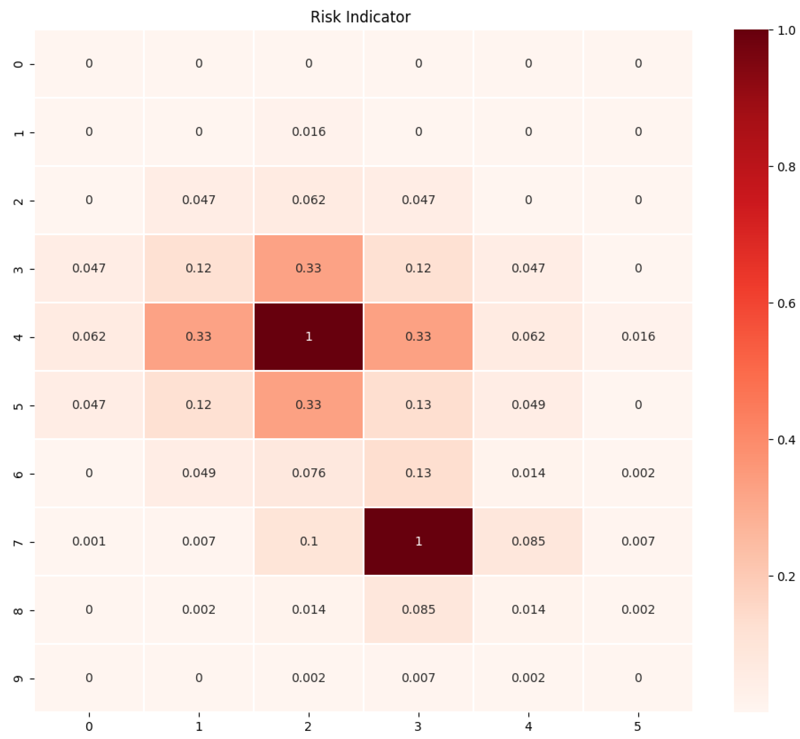
Next, we assigned distinct costs to the two failure states. Specifically, one failure state was designated as having a cost one-third lower than the other. In that scenario, the Risk Indicator was employed. The
Figure 4 presents the results obtained.
5.5. Experiment: Case 4
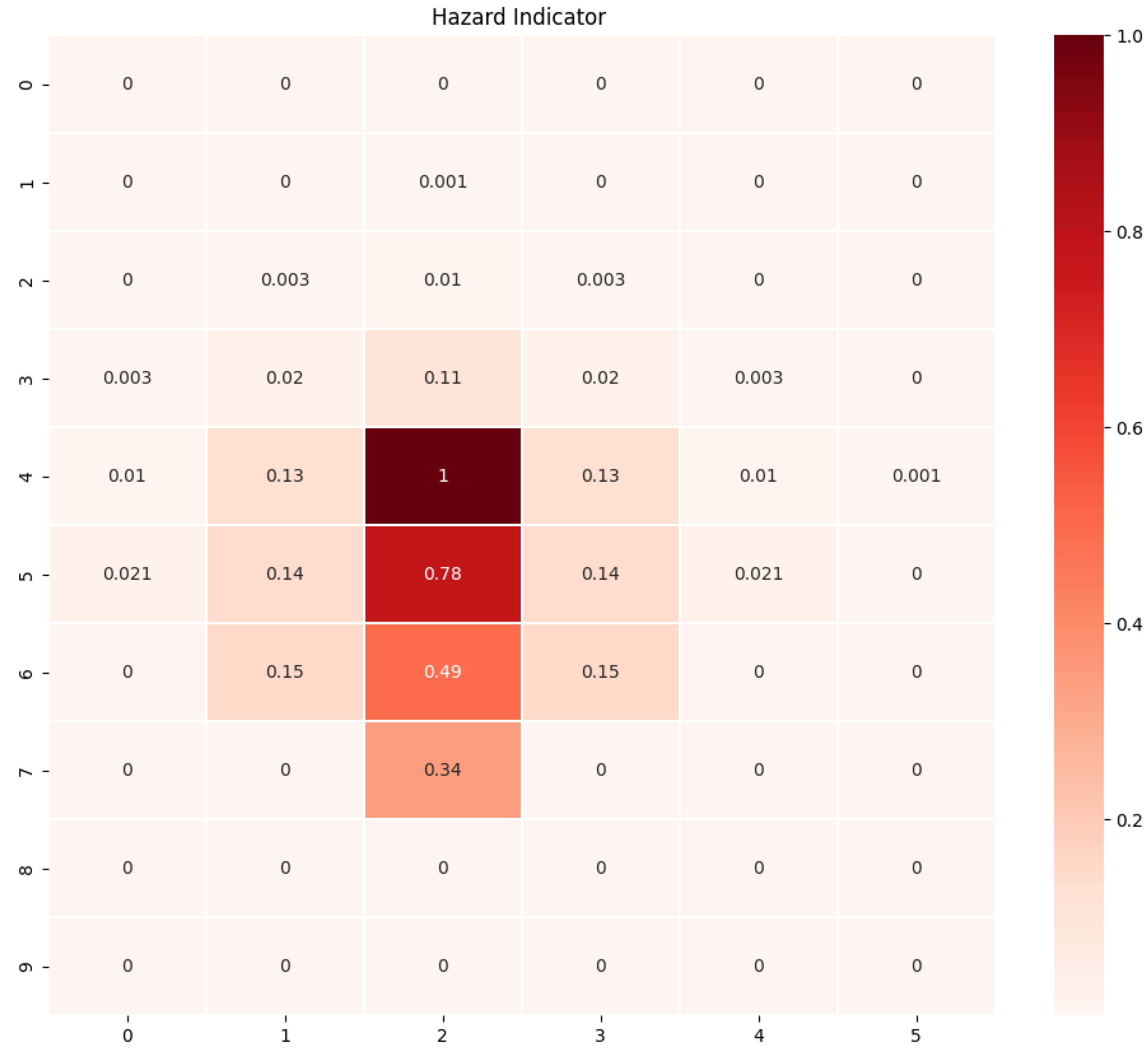
In this experimental session, we altered the probability distribution of actions with a systemic disturbance factor, moving away from a uniform distribution. Specifically, the agent had a 70% probability of moving upward, a 10% probability of moving downward, a 10% probability of moving left, and a 10% probability of moving right. As in the previously examined scenario, we considered one failure state, as presented in
Figure 5.
5.6. Assessment of Experimental Outcomes
We utilized the values of these indicators by experimenting with simulations. Our objective was for the agent, starting from the initial state of the grid at [0, 0], to reach the target state at [9, 4] on the opposite side of the grid, near a failing state, in the minimum number of steps while avoiding fatal situations. We implemented two of the most widely used RL algorithms, with different operational principles: on-policy first-visit Monte Carlo control, and Q-learning one-step (off-policy temporal-difference control), both implemented in look-up-table form and using an epsilon-greedy policy. More in-depth details of these methods can be found in [
4].
During the training phase, the sampling of each action considered the values of the Hazard or Risk Indicators, depending on the scenario. When these values exceeded a predefined threshold (e.g., in experimental case 1, the threshold was set to either or depending on the desired proximity to potential failure states), the sampling switched from the epsilon-greedy exploration strategy (basically, a uniform random exploration in the early steps of training) to a guided mode to avoid visiting high-risk states, remaining in states with the index indicative of lower risk, and effectively creating a path that ensured system safety. This approach significantly influenced the agent’s behavior: by adjusting the threshold levels, it reduced or completely eliminated the possibility of reaching a failure state. Concurrently, an optimal policy for the target was obtained, ensuring the achievement of the desired state in the minimum number of steps while prioritizing safety.
6. Use Case
This section investigates the application of the Hazard Indicator by examining its effectiveness in a real-world scenario: risk management during medical examinations at a Nuclear Medicine Department (NMD). It refers to the practices and protocol implemented within a Nuclear Medicine Department to minimize potential risks associated with the administration of radio-pharmaceuticals for diagnostic procedures. The inherent risk of radiation exposure necessitates close patient monitoring and guidance by nurses during their movements to prevent hazardous situations. For a comprehensive understanding, it is important to acknowledge that the NMD encompasses several distinct locations:
The reception room (RR), where patients are admitted into the department.
The waiting room (WR), designated for patients to wait before the injection of a radio-pharmaceutical.
The injection room (IR), where patients receive the necessary substance.
The hot waiting room (HWR), where patients wait until their radiation levels reach the target range post-injection.
The diagnostic room (DR), where examinations are conducted.
For the medical procedure to be successfully completed, patients must follow this specific sequence: RR → WR → IR → HWR → DR. If a patient deviates from the prescribed sequence, they take a risk of exposure to radioactive agents, which can cause severe injury. Traditionally, nurses ensure adherence to the established procedural sequence during examinations. However, automating this process represents a paradigm shift, transitioning away from the dependence on continuous patient monitoring by hospital staff. To achieve this, various adaptive decision-making controllers, acting as intelligent agents empowered by reinforcement learning algorithms, have demonstrated significant efficacy [
26,
27].
To evaluate the effectiveness of the proposed metric, we employed the system outlined in Shah’s work [
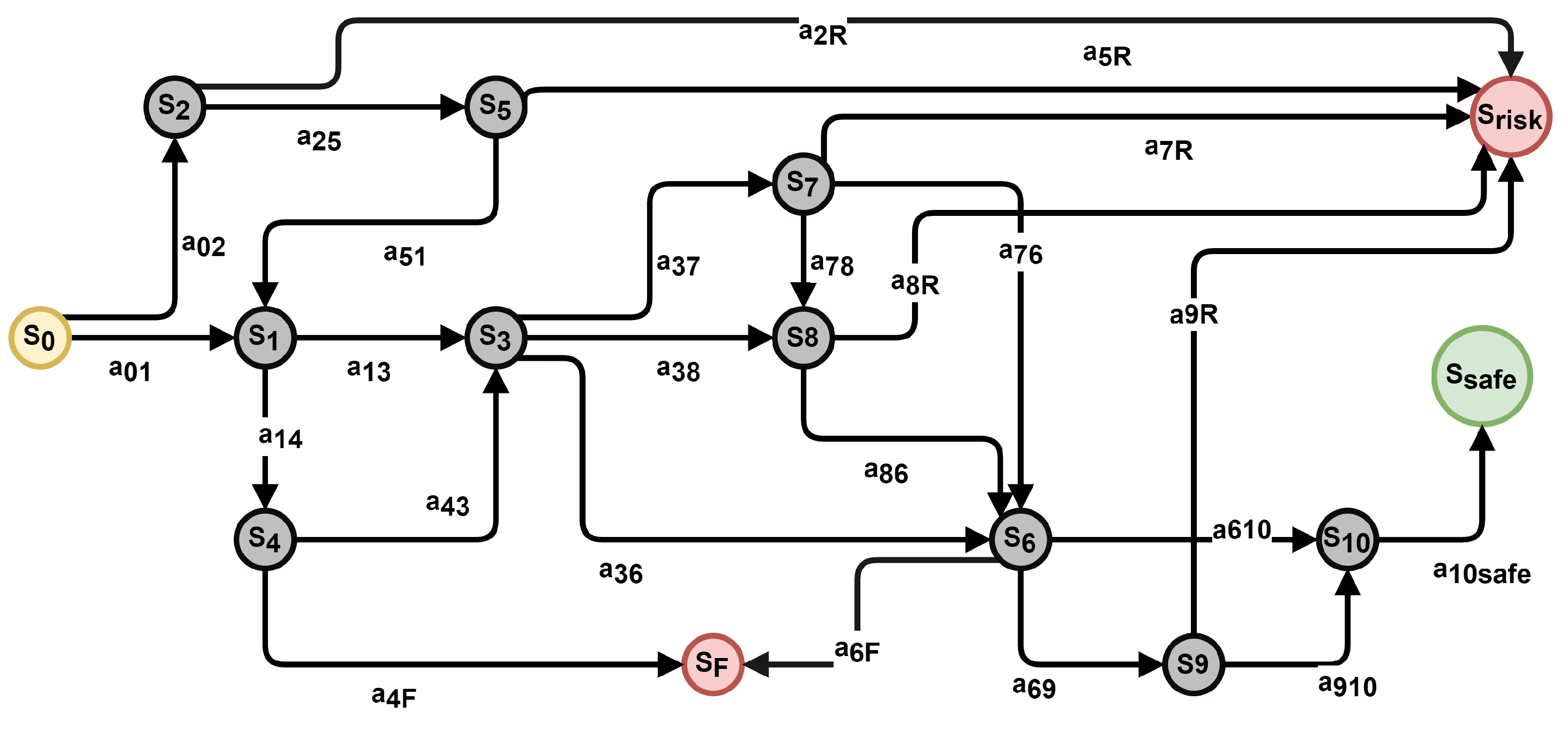
27]. Specifically, the controller utilized RL methods to adapt to the dynamic environment of the examination building. The controller received information about the patient’s current location and based on its learned understanding of the environment subsequently sent guidance messages directly to the patient’s smartphone. A comprehensive description of the employed Markov Decision Process framework is provided in
Figure 6, which illustrates the state–action architecture, and in
Table 1, which provides a comprehensive description of the assumed scenario.
In essence, the environment was modeled with fourteen distinct states, two of which represented terminal states that posed a significant risk to the patient’s safety. Due to these inherent dangers associated with the task and the relatively small number of states, we opted to commence our investigation with an agent restricted to a single action-step, i.e., . Additionally, each action had the same probability of being sampled from those available.
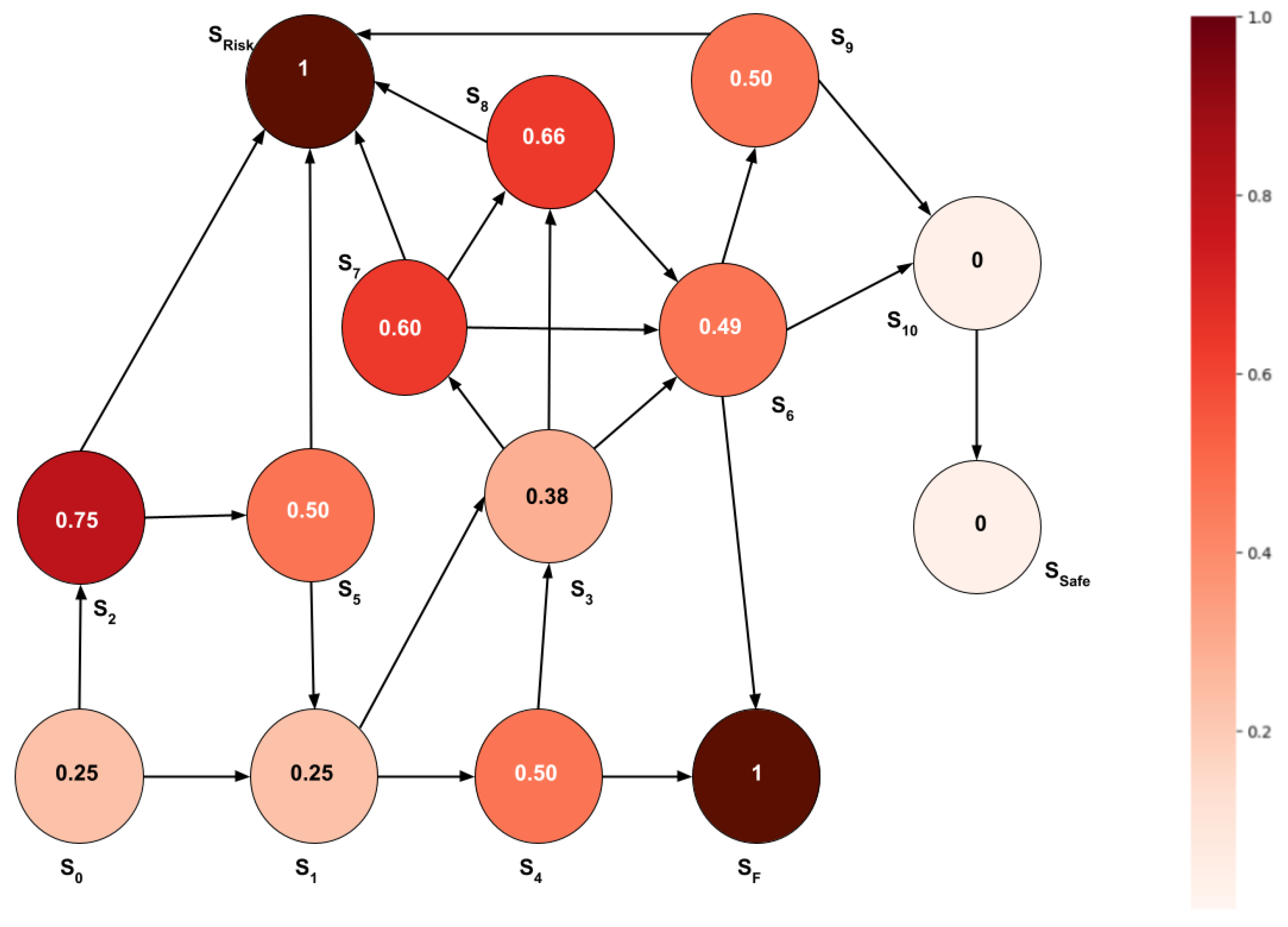
The graph in
Figure 7 depicts the results obtained by employing the Hazard Indicator metric,
, within the scenario described.
The graph in
Figure 7 employs a visual representation where failure states are depicted with a value of one. Conversely, a value of zero indicates safe states. The remaining states are assigned values between zero and one, reflecting varying degrees of hazard.
To further investigate the capabilities of the Hazard Indicator, we expanded the agent’s decision-making horizon by increasing the maximum number of allowable actions from one to two steps, i.e.,
. The results are shown in
Figure 8.
In this scenario, the graph revealed a more nuanced articulation of the Hazard Indicator, capturing a wider spectrum of risk levels compared to the previous scenario.
For our experiments, we constructed the simulated Markovian environment described previously. We employed the same on-policy control algorithm, State–Action–Reward–State–Action (SARSA), utilizing an epsilon-greedy policy implemented via a lookup table, as used in [
27]. A comprehensive explanation of these RL techniques can be found in [
4].
However, we differentiated our approach by integrating the SARSA algorithm with the Hazard Indicator values. We implemented a threshold mechanism that triggered a piloted exploration when the index exceeded a predefined value. By doing so, it ensured the agent remained in states where the Hazard Indicator values confirmed a higher level of safety. Having exploited the SARSA algorithm, we focused on the scenario where . By modulating this threshold, we aimed to manipulate the agent’s exposure to potentially risky situations during training. We investigated the impact of two threshold values: and 0. Only the first one guaranteed a total safe training by preventing the agent from encountering potentially hazardous scenarios. The second threshold, , reduced the frequency of encountering a failure state during training, compared to an algorithm that did not use the index. This approach enabled the convergence to the same optimal policy achieved by the original implementation of the algorithm that did not use safety precautions.
7. Conclusions
This paper introduced a novel metric designed to assess the risk within environments characterized by Markov Decision Processes.
The Hazard Indicator and Risk Indicator proposed in this research offer quantitative evaluations of the risk associated with individual states. These indicators enable agents to prioritize safer actions and interventions based on index values.
While established techniques such as safe exploration methods like shielding rely on predefined safety models, these indicators offer greater flexibility and adaptability across different environments without the need for specific safety rules. Reward shaping and constrained optimization, while effective, often necessitate customization for individual tasks. In contrast, Hazard and Risk Indicators demonstrate greater versatility across a wider range of RL applications. Furthermore, some safe exploration techniques might require complex model training, while these indicators provide a simpler approach to quantifying and managing risk. Therefore, ultimately, their straightforward implementation, highly generalized probabilistic mathematical formulation, and task-independent nature facilitate the RL agent’s comprehension of hazardous states within an environment.
The experiments conducted validated the efficacy of these metrics across various scenarios, elucidating their utility in assessing risk and hazard in complex environments, thereby providing valuable insights for decision-making and risk mitigation strategies across diverse domains.
The primary limitation of these metrics stems from their underlying assumption: a discrete and fully observable state space. In complex environments with continuous or partially observable states, the applicability of these metrics becomes limited. This also poses computational challenges as the number of states increases.
In our future research, we will be actively exploring methods to address these limitations. This includes researching the use of function approximation techniques to refine these metrics and incorporating probabilistic methods to handle partially observable environments. Additionally, exploring the integration of these indicators with a variety of algorithms, beyond those associated with the RL framework, presents a promising avenue for future research.

