Article

Path Planning for Autonomous Mobile Robot Using Intelligent Algorithms

by
Jorge Galarza-Falfan
1,
Enrique Efrén García-Guerrero
1,
Oscar Adrian Aguirre-Castro
1,
Oscar Roberto López-Bonilla
1,
Ulises Jesús Tamayo-Pérez
1,
José Ricardo Cárdenas-Valdez
2,
Carlos Hernández-Mejía
3,
Susana Borrego-Dominguez
1,4 and
Everardo Inzunza-Gonzalez
1,*
1
Facultad de Ingeniería Arquitectura y Diseño, Universidad Autónoma de Baja California, Carrt. Tijuana-Enesenada No. 3917, Ensenada 22860, Baja California, Mexico
2
Instituto Tecnológico de Tijuana, Tecnológico Nacional de México, Tijuana 22430, Baja California, Mexico
3
Instituto Tecnológico Superior de Misantla, Tecnológico Nacional de México, Misantla 93850, Veracruz, Mexico
4
Facultad de Ciencias Químicas e Ingeniería, Universidad Autónoma de Baja California, Calzada Universidad No. 14418, Tijuana 22390, Baja California, Mexico
*
Author to whom correspondence should be addressed.
Technologies 2024, 12(6), 82; https://doi.org/10.3390/technologies12060082
Submission received: 1 March 2024 / Revised: 17 May 2024 / Accepted: 29 May 2024 / Published: 3 June 2024
(This article belongs to the Topic Advances in Mobile Robotics Navigation, 2nd Volume)

Abstract

:
Machine learning technologies are being integrated into robotic systems faster to enhance their efficacy and adaptability in dynamic environments. The primary goal of this research was to propose a method to develop an Autonomous Mobile Robot (AMR) that integrates Simultaneous Localization and Mapping (SLAM), odometry, and artificial vision based on deep learning (DL). All are executed on a high-performance Jetson Nano embedded system, specifically emphasizing SLAM-based obstacle avoidance and path planning using the Adaptive Monte Carlo Localization (AMCL) algorithm. Two Convolutional Neural Networks (CNNs) were selected due to their proven effectiveness in image and pattern recognition tasks. The ResNet18 and YOLOv3 algorithms facilitate scene perception, enabling the robot to interpret its environment effectively. Both algorithms were implemented for real-time object detection, identifying and classifying objects within the robot’s environment. These algorithms were selected to evaluate their performance metrics, which are critical for real-time applications. A comparative analysis of the proposed DL models focused on enhancing vision systems for autonomous mobile robots. Several simulations and real-world trials were conducted to evaluate the performance and adaptability of these models in navigating complex environments. The proposed vision system with CNN ResNet18 achieved an average accuracy of 98.5%, a precision of 96.91%, a recall of 97%, and an F1-score of 98.5%. However, the YOLOv3 model achieved an average accuracy of 96%, a precision of 96.2%, a recall of 96%, and an F1-score of 95.99%. These results underscore the effectiveness of the proposed intelligent algorithms, robust embedded hardware, and sensors in robotic applications. This study proves that advanced DL algorithms work well in robots and could be used in many fields, such as transportation and assembly. As a consequence of the findings, intelligent systems could be implemented more widely in the operation and development of AMRs.

1. Introduction

The current endeavor in mobile robotics is mainly focused on applying artificial intelligence to different levels of the whole robotic system [1]. This includes velocity control [2], instrumentation, sensor fusion [3], object recognition, etc. However, path planning is a particular task that broadens the reliability of any robot, simplifies the interaction with a human operator, and, ultimately, is common to all types of autonomous robots [4], not only mobile robots. There have been plenty of methodologies proposed to solve path planning [5], including the traditional model-based planners such as the Artificial Potential Field (APF) method, cell decomposition, the dynamic window method, etc. [6]. These algorithms are the classic approaches to controlling the motion of most of the first mobile robots. Although traditional methods are reliable, they require constant recalculations, leading to considerably high processing and computation times. The first experiments for the solution of robot path planning through heuristic approaches date to the late years of the 1960s [7], at the Stanford Research Institute, where ref. [8] developed “Shakey”, an autonomous robot that navigates using the A* intelligent algorithm. In the following years, the Jet Propulsion Laboratory of the National Aeronautics and Space Administration (NASA) designed and released a series of semi-autonomous mobile robots called “Rover” that specialized in exploration for space missions, and by 1977, they were working on the possibilities of using machine learning in the exploration of unknown environments [9]. In concordance with the previous context, heuristic approaches grant a deeper exploitation of environment data to expand the robot’s adaptability and avoid potential collisions [10]. In recent years, a learning-based approach that has gained popularity is Reinforcement Learning (RL) [11]. It consists of a series of Artificial Neural Networks (ANN) that are used to update a learning model based on a reward function applied to the potential action or maneuvers of the robot [12]. One of the main reasons behind the popularity of this methodology is that it is based on trial and error, which is parallel to the biological way of learning. Moreover, the trained model is highly operational in different non-deterministic situations, like unknown dynamic obstacles [11]. RL is a promising tool, but its real-world implementation is not trivial. Although simulation is a reliable way to compare and benchmark the different versions that have been proposed, there still exists a bridge between theoretic algorithms and real-world environments [13].
On the other hand, learning-based navigation requires a specific set of characteristics and specifications for the robot that could grant the proper execution of many complex tasks and algorithms simultaneously. For this reason, hardware will define the robot’s functionality, level of flexibility, and potential limits. The primary sensors used as the input data and feedback for the RL controller are LiDAR, IMU, ultrasonic radar, and one or multiple cameras [13]. Sensor data are used as the perception elements for navigation. Specific features are extracted from the input data and analyzed, looking for all the possible generalizations in the robot’s environment dataset that could potentially guide the RL algorithm’s decision making [14]. These generalizations provide information like the safe distance between the robot and walls or obstacles, potential risks when applying a specific action policy, etc. The focus on RL is due to the worldwide interest in applying intelligent and learning algorithms and methodologies like machine learning (ML) and deep learning (DL) in industrial environments. Although different alternatives have been successfully used, intelligent systems report positive results and adaptability to the constant evolution of embedded systems and state-of-the-art computers because there is a clear benefit of improving the ML processing tasks using distributed CPU and GPU processing [15]. RL is prone to return various results depending on the decided balance between exploration and exploitation. These features in RL algorithm variations make this methodology reliable in different situations and environments.
New possibilities for learning-based path planning are discussed in [16]. The author suggests that the contribution of more than one sensor could improve the learning process, and at the same time, it would benefit the performance of mobile robots in real-world scenarios. Moreover, [17] addressed the potential of deep RL to help deploy robots to navigate uncertain environments.
YOLO (You Only Look Once) version 3 is an enhanced object identification algorithm built on YOLO9000. YOLOv3 can achieve an average accuracy with a faster detection speed compared to one-stage neural networks, with a clear speed advantage over algorithms like HOG (Histogram Oriented Gradient). YOLOv3 has 3 × 3 and 1 × 1 convolutional layers. It is known as darknet53 since it uses 53 convolutional layers. YOLOv3 simultaneously employs several independent logistic regression classifiers. Binary cross-entropy loss forecasts the classification during training [18]. Another critical aspect of YOLOv3 is that it uses k-means clustering non-supervised training to predict the bounding boxes of the detected objects. The algorithm has three defined scales for the bounding boxes, with nine clusters. Then, the exact bounding box size is calculated using the detected object’s scales and centroid [19].
It is essential to note the importance of finding a valid route or path and choosing the less expensive one in terms of time and energy consumption. In 2022, two investigations were published on Unmanned Aerial Vehicle (UAV) path planning using a Q-learning-based algorithm. Ref. [20] proposed a static environment path planner that can estimate the most efficient route from any position in the map, considering UAV energy limitations and safety. Ref. [21] worked on applying UAVs in a mobile edge computing network, using DRL to evaluate and organize the priority of its tasks, considering the duration of flight and battery capacity.
This article proposes a method for developing an Autonomous Mobile Robot (AMR), with the study basing the experimentation on state-of-the-art research. This method integrates Simultaneous Localization and Mapping (SLAM), odometry, and artificial vision based on deep learning, providing a reliable solution for path planning through open-source software utilities like ROS and the embedded system NVIDIA Jetson Nano. These characteristics are crucial for the execution of subsequent autonomous tasks. In addition, this study intended to assess the performances of two convolutional neural networks in the scenario of AMR path planning and propose a method of using a vision system to identify potential obstacles and communicate it to the navigation path planner that runs locally on the robot’s computer.
The rest of this paper is organized as follows. Section 2 describes the most relevant works and recent contributions to developing learning-based AMRs. Section 3 presents the materials and methods for the design and experimentation with the proposed AMR. Section 4 presents the results obtained during the experiments. Section 5 explains and discusses the results. Finally, Section 6 summarizes the conclusions of this study.

2. Related Work

2.1. ROS Autonomous Mobile Robots

The Robot Operating System (ROS) is an open-source tool for developing a wide variety of robotic systems grouped into mobile and fixed types. Whether the robot is one type or the other requires general software capabilities, such as communication with external devices, updated libraries and packages, and an accessible programming environment [22]. Another critical aspect of the ROS is its growing impact on professional and academic robotics since there are updated open-source packages and accessible examples online [23].
In [24], the authors integrated LiDAR navigation and path planning using a laptop as the ROS controller and a Raspberry Pi embedded system as the ROS agent. This investigation proved the limitations of LiDAR, as its location is critical to obtaining an accurate representation of the environment and the objects close to the robot. Also, the author suggests using an online user interface to control the ROS topics and nodes easily.
In [25], the authors proposed an RL-based method to autonomously navigate with no map using the simulator ROS simulator Gazebo. The author expects the method to be applied in real-world inspection tasks.
As suggested in the addressed works, the ROS is a system commonly seen in most robotics projects, from some minor functionality to being the central system that integrates all the robot subsystems [26]. However, the cited works did not process environment image data in real time to help the navigation system.

2.2. Learning Algorithms

In [27], the authors addressed using a method to modify how to update the reward and expected reward tables, enabling the possibility of transferring learning data between multiple agents, called “collaborative navigation”. In recent years, the authors have published three more papers on collaborative learning and fuzzy logic applied to mobile robotics.
The authors of [28] emphasized advancements in deep reinforcement learning (DRL) applied to mobile robotics. DRL is a methodology that combines RL with Neural Networks to extract essential features directly from the agent or robot’s perception system, including cameras, raging sensors, and more. Conventional RL, on the contrary, requires defining specific features to update the learning tables or matrices. The critical difference between both methodologies is analogous to the difference between machine learning and deep learning. The authors have additionally worked on obstacle avoidance strategies along with DRL. They used a DRL model called D3QN, modified the learning rate batch size, and introduced a layer normalization function to process images from the robot’s camera. These changes reduce the learning process time, leading to a better reaction to obstacles [28].
The study discussed in [29] introduced a deep reinforcement learning algorithm called DDQN. It introduces 2D LiDAR data in the reward system to obtain feedback from the environment after each robot action. The experiments showed a better performance in non-obstacle navigation.
The authors of [30] developed a method for path planning using a deterministic policy gradient and a sequential linear path planning algorithm to achieve planning in larger maps, contrary to previous RL limitations.

2.3. Investigation Tendencies

Given the context explained in the Introduction section (Section 1), the integration of RL and path planning dates to the early 1990s [31].
In making a comparison to the volume of publications in the “RL applied to AMRs” field from the last ten years, as shown in Figure 1, it is clear that there has been a considerable increase in interest from 2019 to the present, arguably caused by the recent popularity of deep learning systems and the improvement of the available hardware, including better multi-core processors and GPU-based learning tools and libraries.
Figure 2 shows the connections between 786 keywords in the Scopus data. It is limited to the keywords with a minimum occurrence of 5, which allows the map to read much easier, containing only the 40 most relevant and connected keywords. It was generated using the open-source tool VOSviewer [32]. The diagram indicates the proximity between the keywords based on their frequency in the database. The keyword “reinforcement learning” had a total of 82 occurrences and is closely related to “obstacle avoidance”, meaning that RL methodology is constantly applied to that specific task; the D3QN Network [28], the simulator proposed in [33]; and the motion strategy from [2].
The second most connected keyword was mobile robots, with 63 occurrences. It concerns many different types of mobile robots, not just AMRs. Moreover, Q-learning is the only algorithm present in the diagram, possibly meaning that it is the most general RL algorithm. Finally, the keyword “motion planning” had 59 occurrences, the third most connected. RL has a much broader application spectrum, apart from path planning.
Another essential comparison provides more profound knowledge about the sources of the papers related to the research topic, because the analysis of such information explains the global context of the RL and DL investigation. Countries with a higher interest in such technology and methodologies are willing to invest more funds and effort to implement more learning-based algorithms for actual industrial applications supported by an economic benefit. The country with the most documents in the Scopus database is China. It is a country that has contributed some of the most cited and relevant papers in the last five years. Some of the topics from such investigations are improvements to RL algorithms that solve global navigation problems and navigation through unknown environments. IEEE Robotics and Automation Letters is the journal that has released more papers on the topic in the last few years. Some of those papers include [34], which introduces a path planning approach called GR2L tested in multi-robot tasks; the previously addressed simulator proposed in [33], and the application of RL in instrumentation research in [35]. Ref. [36] suggested a method for conducting a hierarchical exploration in crowded environments, and Ref. [37] presented a method to make a quadruped legged robot adapt to external conditions through RL.
Another journal with important contributions is Sensors from MDPI. In recent years, some papers are [38], which introduces a deep Q-network for using LiDAR data to generate discrete actions; [39], which applied a method called Hindsight Experience Replay to mitigate the sparse reward problem; and [40], which presented a technique for calculating the best path in environments with multiple robots. Their main focus was path planning in wider environments, obtaining more reliable probability tables [41].

2.4. Hardware Comparison

According to Table 1, most recent investigations have applied GPU-based processing, with NVIDIA RTX and GTX being the most popular ones. However, many simulations are being performed on CPUs, especially Intel Core i5 to i9. The studies that ran tests on natural environments and agents use mostly the embedded system Raspberry Pi 3, with remote communication to a computer that processes the learning algorithm. According to the literature revision, most experiments are limited to simulations using software like Gazebo from the Robot Operating System (ROS) [42].
Despite the successful results obtained in the cited works shown in Table 1, there are the following limitations:
  • Only a few articles mention an actual implementation of the trained algorithms on embedded systems [41].
  • There is a lack of research about training the CNN model on an embedded system, as it simplifies the integration, reduces costs, and adds portability. NVIDIA Jetson Nano is an option for centralizing the AMR processing.

3. Materials and Methods

The following section describes the methodology for building the robot’s structure, as well as the selection of all the materials used. The components’ distribution was designed to allow further modifications and maintenance. The power supply is split for separate module inspection and safety reasons. Also, the prototype was constructed vertically, mounting the modules on top of each other. The selected sensors, such as the encoders, LiDAR, and IMU, were included for their simplicity and reliability. Other sensors could be added to increment the accuracy in navigation and reduce motion error.

3.1. Materials

The proposed robot is based on the JetBot ROS AI development kit from Waveshare. The main hardware components were kept. However, with its corresponding structural modifications, the power supply module was modified to allow the addition of a second battery dedicated exclusively to supplying energy to the two motors and the rest of the sensors connected to the microcontroller.
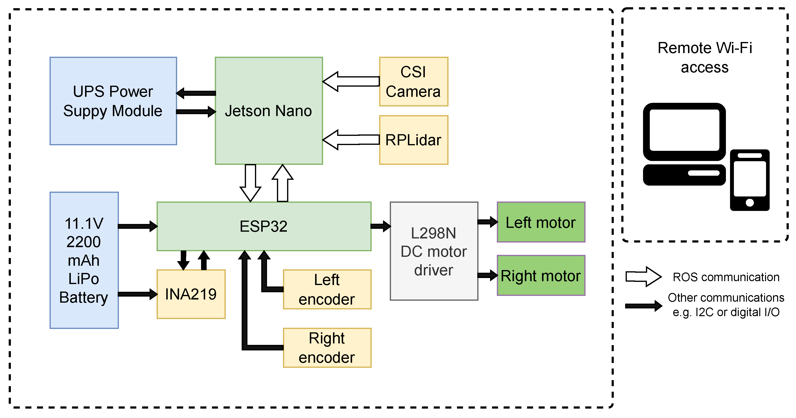
Figure 3 illustrates the connections and communication between the robot modules starting with the batteries on the left, the embedded system at the center, and their input sensors and outputs indicated by the arrows’ direction. This section enumerates the hardware devices present in the robot structured as seen in Figure 3.
  • Jetson Nano
    This embedded system from the manufacturer NVIDIA works as the central computer that performs all the important calculations, deep learning training, and remote communication through the operating system ROS. Jetson Nano has a GPU with 128 CUDA Cores, enabling the robot to run real-time object recognition through a deep learning model. This cognitive independence is fundamental to reaching a correct level of autonomy for the robot.
  • ESP32
    This is a development kit from Espressif Systems. It has a dual-core, 32-bit microprocessor and performs better than other low-cost microcontrollers. The embedded system establishes serial communication with this device as it continuously reads the two encoders and other sensors alongside the PWM output control of the two direct current (DC) motors.
    Another important characteristic of ESP32 is its connectivity simplicity, as it has Bluetooth and Wi-Fi communications, which is particularly useful for the remote control of the robot. However, the communication to Jetson Nano is serial through a USB port of the embedded system.
  • Motors
    The motors in the JetBot development kit, also from Waveshare, are regular 12 VDC brushed motors coupled with a gearbox with a gear ratio of 30:1 that provides enough torque for the robot to move smoothly in most indoor environments.
    The robot’s locomotion is differential, requiring two controllable wheels and two non-controllable caster wheels. This design provides better stability to the robot than a single caster wheel. However, the friction added could cause difficulty in moving in certain situations.
  • Sensors
    Each DC motor has a 2-channel encoder mounted directly on the shaft. Given the properties of the gearbox described earlier, the encoder is used to read the position and velocity of the robot inferred from the local movement of the left and right wheels. Each encoder provides 330 pulses per revolution. Since the motor has two separate channels to read the pulses, it is possible to track the direction of the local movement of the two wheels.
    However, the sensor that is more appropriate for estimating the robot’s position is RPLidar from the manufacturer Slamtec. It is a rotative device that emits an IR light beam read by a sensor to estimate the distance between the sensor and its surroundings.
  • Camera
    The camera in the prototype kit is a IMX219-160 CSI manufactured by Waveshare for Jetson Nano or Raspberry Pi. It has 8 MP of resolution and an angle of view of 160 .
  • Batteries
    As briefly explained, the battery module was modified to increase the robot’s autonomy level. The original battery module of the JetBot ROS AI kit is equipped with three 18,650 rechargeable 3.7 V, 9900 mAh batteries in series that power the whole hardware, including the embedded system, the microcontroller, and the motion system. The batteries are from the manufacturer GTL Everfire.
    Working with a single battery could cause potential difficulties, mainly because it limits the autonomy of the robot and its ability to stay powered for long periods. Based on the information of the manufacturer, any mishandling of the battery can cause a fault in the embedded system. And due to the interest in working with the robot’s autonomy, it is important to grant the safety of the modules, as shown in Figure 3.
    The uninterruptible power supply (UPS) module provides energy to Jetson Nano. It includes four 18,650 batteries and their respective protection and monitor circuits. The communication between the UPS battery module and Jetson Nano is through I2C protocol.
    The second battery is an 11.1 V, 2200 mAh LiPo battery produced by Floureon. It is suitable for different autonomous robots like drones [47]. This battery helps to isolate the control system from the rest of the hardware. It grants safety, it is a reliable solution to possible communication difficulties, and it elongates the working time of the embedded system, which constantly communicates remotely.

3.2. Methods

This section focuses on the proposed method to make the robot interpret and interact with its surroundings through movement. The complex tasks involved, such as artificial vision, object recognition, SLAM, and motion control, are run by independent ROS nodes. This makes the modification and debugging of each task easier. Moreover, some of them are required in specific situations; therefore, the robot can work with the bare necessary modules to prevent unwanted waste of energy.

3.2.1. Robot’s Cinematic Model

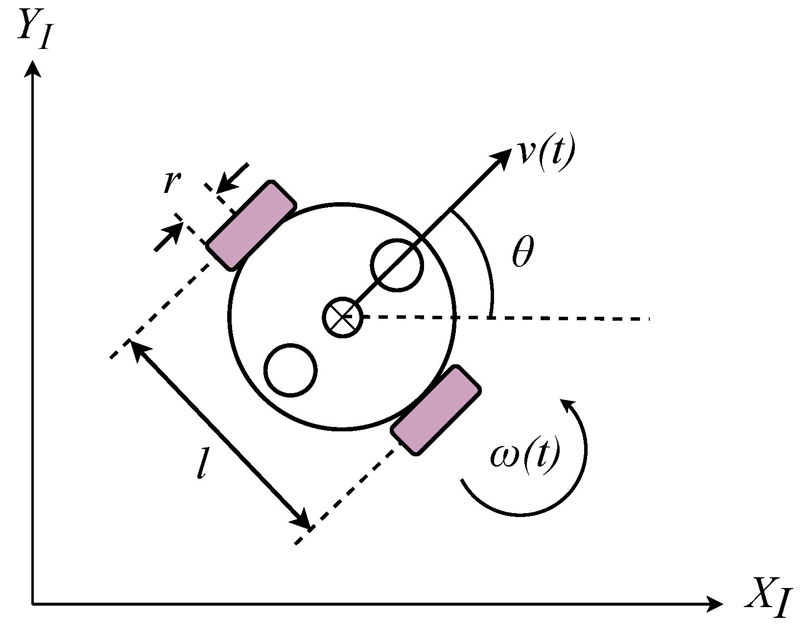
Figure 4 shows the global coordinate system depicted as X I and Y I , also known as the inertial system. It consists of the axes that define the environment or map in which the robot moves. Since the differential mobile robot moves in a two-dimensional space, the correct way to analyze its movement is with a two-dimensional rotation matrix that helps to define the robot’s linear velocity v ( t ) and angular velocity ω ( t ) , as shown in Figure 5.
The local coordinate system ( X R , Y R ) shown in Figure 4 is defined to analyze the motion produced by the robot’s two wheels relative to the chassis’ center point P, which is considered a position reference point in the global coordinate frame ( X I , Y I ) . With this coordinate system ( X R , Y R ), it is possible to separate the wheels’ motions produced by their angular velocities ϕ ˙ r and ϕ ˙ l and relate them to the overall movement of the robot in the global coordinate frame ( X I , Y I ).
In assuming that the robot starts moving from the position depicted in Figure 4, with orientation θ measured counter-clockwise from the X I -axis, Equation (1) defines the rotation matrix:
R ( θ ) = c o s θ s i n θ 0 s i n θ c o s θ 0 0 0 1 ,
where R ( θ ) is the rotation matrix.
Since the mobile robot interacts with its surroundings using its two controllable wheels, it is possible to describe the movement of the robot with a cinematic model that relates the robot’s motion ξ ˙ R in the local coordinate frame with the motion ξ ˙ I in the global coordinate frame (Equation (2)).
ξ ˙ I = R ( θ ) ξ ˙ R .
where the variables are defined as follows:
  • ξ ˙ I is the robot’s velocity in the global coordinate system ( X I , Y I );
  • ξ ˙ R is the robot’s velocity in the local coordinate system ( X R , Y R ).
Equation (2) represents the model of the differential drive robot, defined by the rotation matrix R ( θ ) multiplied by the robot’s local velocity vector ξ ˙ R , which includes linear velocity v ( t ) and angular velocity ω ( t ) .
About Figure 4, the robot cannot move along the Y R -axis due to the perpendicular orientation between this axis and the wheels. Therefore, under this consideration, the y-component of the velocity vector ξ ˙ R can be nullified, as shown in Equation (3).
ξ ˙ I = R ( θ ) ξ ˙ R = c o s θ s i n θ 0 s i n θ c o s θ 0 0 0 1 v ( t ) 0 ω ( t ) .
where the variables are defined as follows:
  • v ( t ) is the linear velocity in the robot’s local X R -axis;
  • ω ( t ) is the robot’s angular velocity around the Z-axis.
The linear velocity v ( t ) and angular velocity ω ( t ) can be expressed regarding the robot’s specific measurements and the wheels’ angular velocities ϕ ˙ r and ϕ ˙ l , as shown in Equations (4) and (5).
v ( t ) = r 2 ϕ ˙ r + ϕ ˙ l .
ω ( t ) = r l ϕ ˙ r ϕ ˙ l .
where the variables are defined as follows:
  • r is the radius of the left and right wheels;
  • l is the distance between the left and right wheels;
  • ϕ ˙ r is the angular velocity of the right wheel;
  • ϕ ˙ l is the angular velocity of the left wheel.
Equation (6) is obtained by solving the product of Equation (3) and substituting v ( t ) and ω ( t ) with Equations (4) and (5). This equation helps to relate the robot’s movement in the global coordinate system (the environment) and the movement of the two wheels.
ξ ˙ I = r ( ϕ ˙ r + ϕ ˙ l ) 2 c o s θ r ( ϕ ˙ r + ϕ ˙ l ) 2 s i n θ r ( ϕ ˙ r ϕ ˙ l ) l = x ˙ y ˙ θ ˙ .
where the variables are defined as follows:
  • x ˙ is the linear velocity in the global X I -axis;
  • y ˙ is the linear velocity in the global Y I -axis;
  • θ ˙ is the angular velocity around the global Z I -axis.
Figure 5 displays the direction of the linear velocity v ( t ) , angular velocity ω ( t ) , and the parameters of the robot r, l, and orientation θ described previously [48].
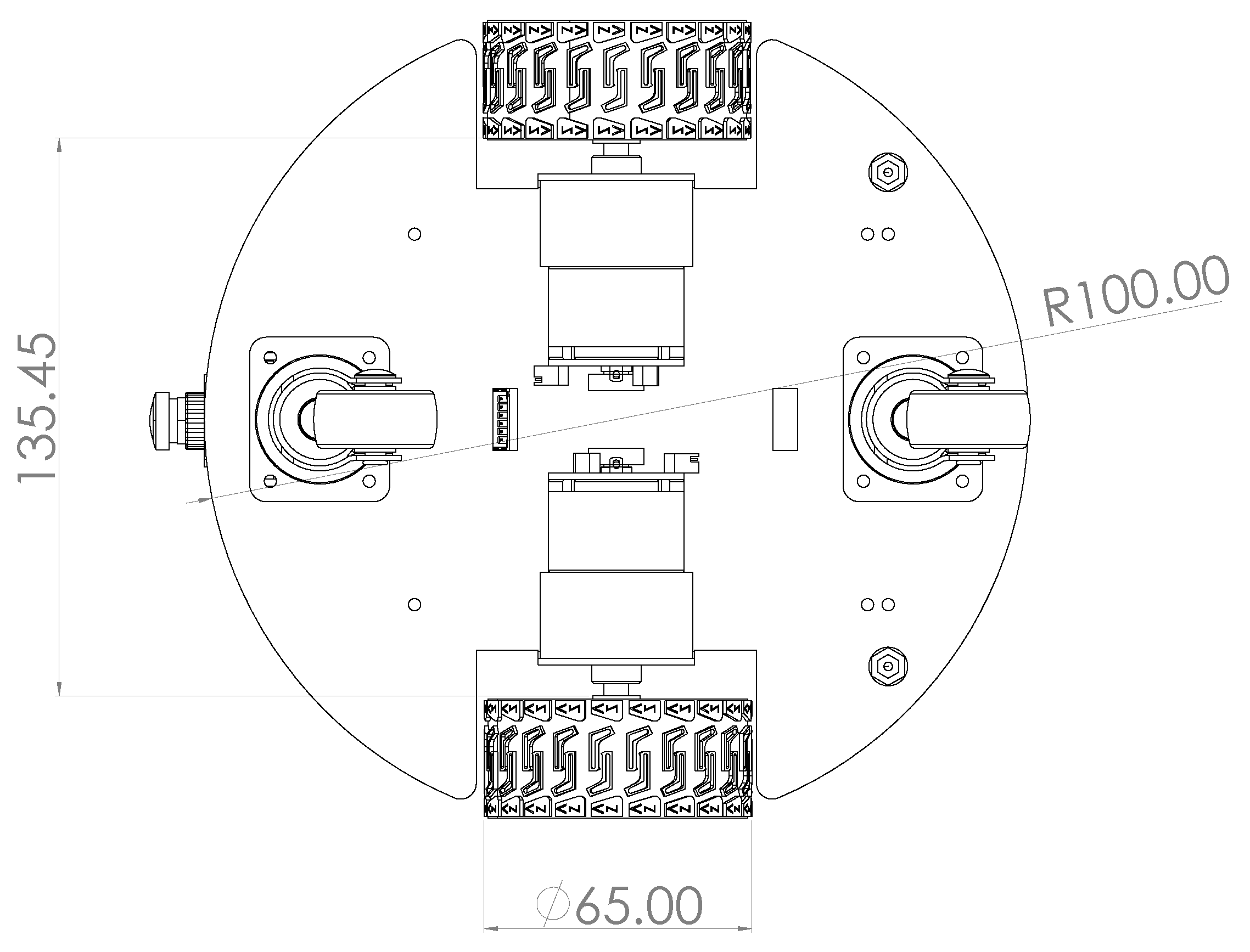
Figure 6 depicts the bottom view of the proposed robot. The first specification that has to be addressed is the robot’s mechanic structure. As detailed previously, the robot’s locomotion setup is differential and stabilized with two caster wheels. Figure 6 shows an accurate drawing that displays the bottom view of the robot with its dimensions and the locations of the four wheels.

3.2.2. Path Planning Algorithm

This study selected the Adaptive Monte Carlo localization algorithm (AMCL) for robot localization [49]. AMCL operates through a particle filter, employing a predefined configuration for the sampling procedure and assigning significance weights to individual particles. When provided with a known map, the AMCL algorithm estimates the robot’s pose as it traverses it and gathers environmental data through range and odometry sensors. Each particle within the algorithm signifies a potential robot pose, thereby reflecting the distribution of feasible states. AMCL requires less memory as its memory usage correlates directly with the number of particles and remains constant irrespective of map size expansion. In AMCL, the primary factor influencing the localization’s efficacy is the quantity of particles. This study set the particle count at 1000, which was later adapted, striking a favorable balance between localization accuracy and speed.
Figure 6. Bottom view of the robot (units are in millimeters).
Technologies 12 00082 g006
Furthermore, the default values for other control parameters were adopted from the ROS navigation package [23]. Because the navigation configuration favors the built map over LiDAR data, the proposed AMR perceives the objects within the map. Consequently, the path planner generates a longer collision-free route to circumvent these objects.

3.2.3. Velocity Controller

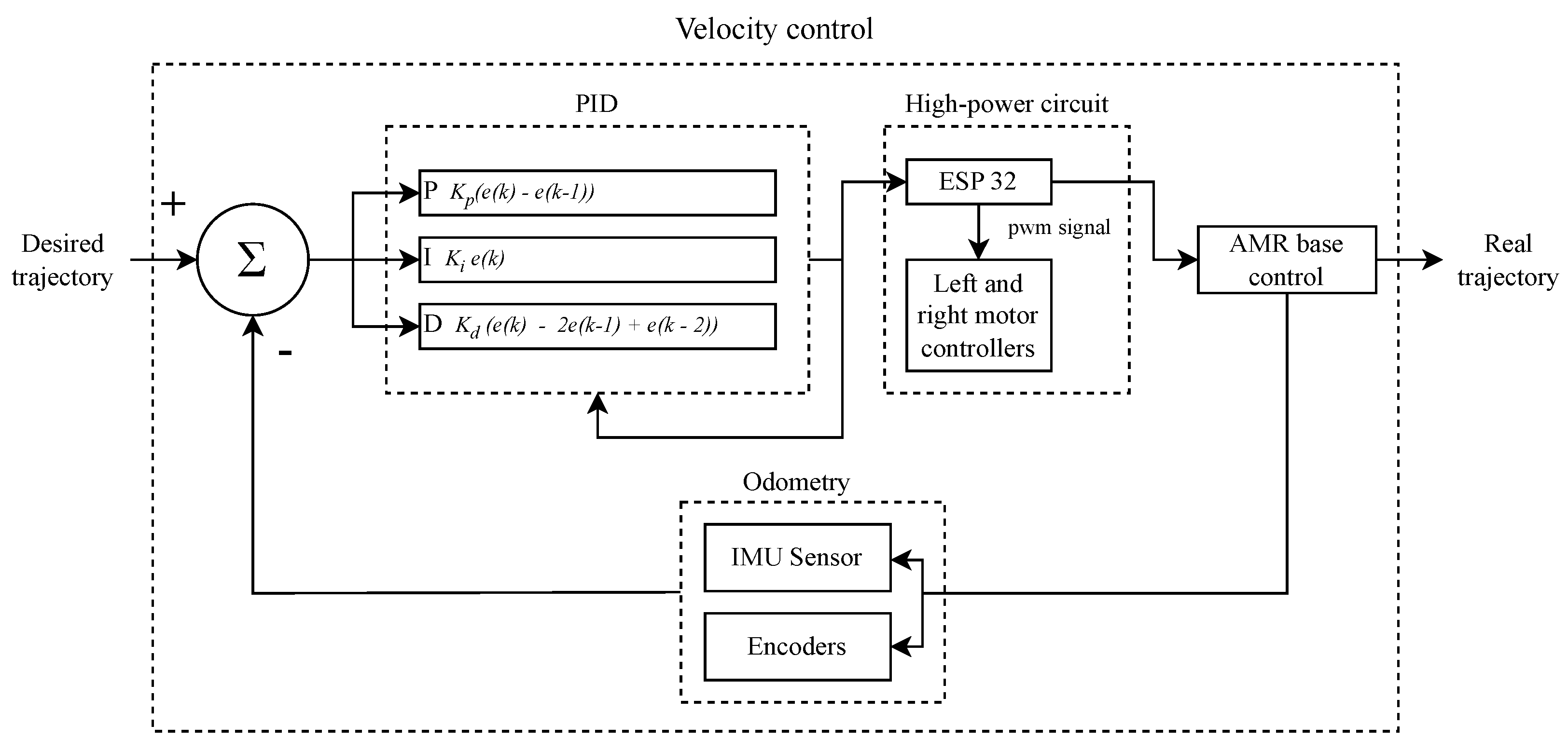
Figure 7 depicts the additional controller used to adjust the velocity output signal of the proposed AMR that makes its base move. Therefore, the base control represents the actual movement of the robot, which is different from the desired or predicted motion.

3.2.4. Differential AMR’s Base Control

The ROS runs in the Jetson Nano and is the central controller. Every major decision is made from it, and it can access all the variables (ROS topics). Since the ESP32 microcontroller interacting with the inputs and outputs is a separate module, it must communicate with Jetson Nano through the serial port using the node rosserial.
Figure 8 shows the location of the rosserial node and its topics. These topics are published and are therefore read from the embedded system. The node teleop generates the velocity command during teleoperation, which is the remote control of the robot via Wi-Fi to move the base during mapping and set-up. The basic topic that controls the robot’s movement is cmd_vel, a generic topic from the ROS that contains a twisting command for the robot in its global coordinate system. It includes movement commands for the global X-, Y-, and Z-axes and rotation around each of them, resulting in a total of 6 axes. Since JetBot is a differential-type robot moving on an indoor flat surface, it does not move along the Z-axis, and it rotates only around the Z-axis and not in X or Y. The global velocity command is read in the microcontroller and processed to generate a PWM signal that is then sent to the motors’ drivers, ultimately causing a movement of the robot’s chassis. The AMCL planning system runs in the embedded system Jetson Nano and generates the cmd_vel from its ROS node called amcl.
Furthermore, Figure 8 shows a graphic representation of the ROS nodes running when the robot moves autonomously. The PWM signals pwm_right and pwm_left result from the microcontroller’s processing of the movement command. This requires converting the motion command given in terms of the global coordinate system (in the axes X and Y, and turns around in Z) to the robot’s local coordinate system (movement in the X-axis and turn around in Z). This conversion requires an algorithm to balance the velocity variations in the two motors. The encoders’ signals are read directly from the digital interrupt inputs of the ESP32 microcontroller. These ticks accumulate in local variables and are published through rosserial. Each encoder has two channels, so the counters can also decrease to add the possibility of tracking the exact position of each differential wheel. LiPo battery monitoring is performed by reading the INA219 current sensor using the I2C protocol. Then, these data are shared with Jetson Nano as a ROS topic.

3.2.5. Environment Mapping

In addition, Figure 8 also includes the RPLidar node. It works through serial communication between the device and Jetson Nano. The sensor scans the environment, and the hector_mapping node generates a map based on the movement of the motor with a starting point as a reference. To create a map, it is important to run the mapping algorithm while the robot moves using the textit/teleop node. The Hector SLAM algorithm ROS package allows for generating a map in yaml and geotiff formats. It is important to mention that the mapping process can be monitored using the ROS Rviz tool because of the robot’s reduced velocity of approximately 0.05 m/s during the mapping process.

3.2.6. Artificial Vision

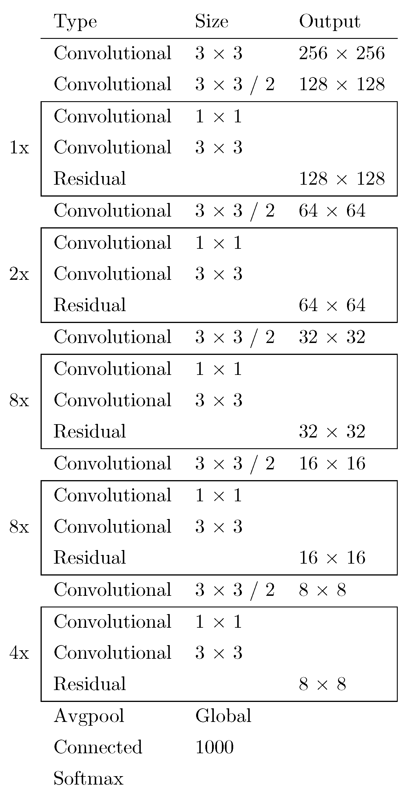
The proposed DL real-time obstacle detection models are YOLOv3 and ResNet18, and their architectures are shown in Figure 9 and Figure 10, respectively. These were tested to find the best-performing model within the main system.
YOLOv3 was selected due to its robustness and compatibility with Jetson Nano. Figure 9 depicts its architecture, serving as the primary CNN model for obstacle detection in the environment. This CNN model was selected for its ability to detect the obstacle’s dimensions and location within the AMR’s field of view. The YOLOv3 model must be manually installed on the Jetson Nano embedded system for execution on a ROS node (see Figure 8).
After installing and setting up a trained YOLOv3 model with its respective weights, the algorithm can recognize objects read from the robot’s integrated camera. Then, the tool can be implemented to recognize potential obstacles in the robot’s near path. We propose using a dataset with two classes to train the DL models for obstacle detection. In the lower section of Figure 8, the DL model (YOLOv3 or ResNet18) is represented as a node of the ROS working simultaneously with the rest of the control system.
Figure 10 depicts the ResNet18 architecture, serving as the secondary CNN model for obstacle detection along the path. Its selection is based on its favorable performance in previous real-time artificial vision assessments within embedded systems. This DL model is also available in the firmware version of the proposed robot JetBot ROS AI [50].
The ResNet18 CNN uses the Pytorch and Torchvision libraries through transfer learning. Table 2 shows the hyperparameters used for the training.
The dataset created for the training was separated into two classes: blocked and free. The first class includes 306 images, and the second one, 328 images with size 224 × 224 pixels. The training process results are summarized in Section 4.
Figure 10. Architecture of ResNet18 CNN, taken from [51].
Technologies 12 00082 g010

4. Results

The results shown here are split into hardware and software because there is relevant information for both groups; therefore, separating them helps to define the diverse functions of the robot’ performance.

4.1. Hardware Implementation

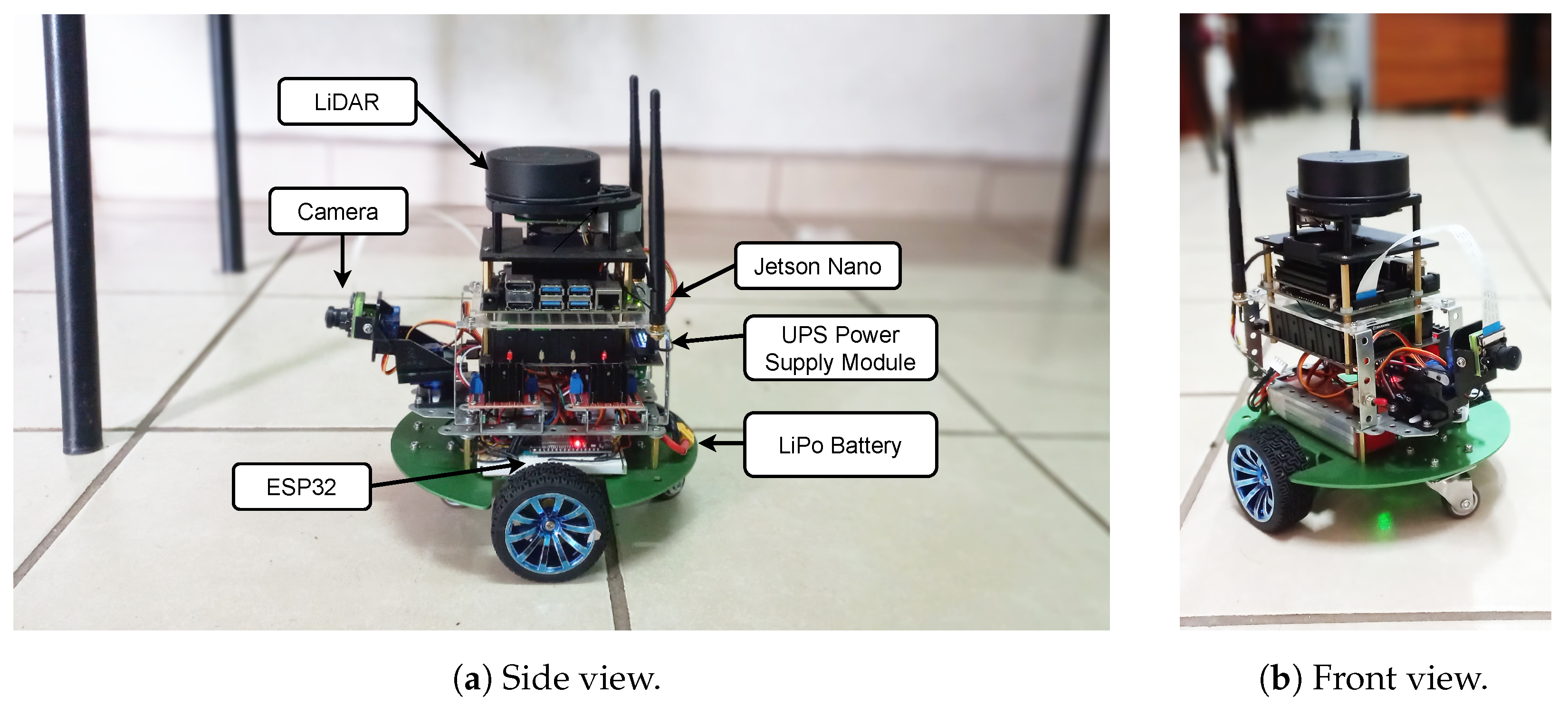
Figure 11a is a side view of the robot in the laboratory where the experimentation occurred. As indicated with the labels, ESP32 is located in the lower section, and LiPo battery is placed next to it, as both are related to the motors’ power circuit. Jetson Nano is in the upper section of the robot, as it interacts mainly with the LiDAR, digital camera, and the UPS power supply module, as depicted in Figure 11a.
Figure 11b is a front view showing some of the modifications made to the base prototype. Starting from the lower section, there are the locomotion system, the control devices, and the LiDAR at the top. In the front, there is the digital camera. The current arrangement of the hardware devices results from multiple iterations during the development process, and it is adaptable to further improvements. One improvement is upgrading the battery module, originally packed with a three-battery power module. It was replaced with a four-battery module for the embedded system and sensors, and an additional LiPo 12 V battery for the DC motor locomotion system. This modification to the power system is due to the importance of battery autonomy. Another modification is the addition of a microcontroller ESP32 to generate the PWM signals for the DC motor drives. This simplifies the addition of multiple sensors, like the motor’s encoders and the LiPo battery current monitor sensor.
The maximum autonomy time for the embedded system powered the by 8.4 V UPS module is approximately 4 h, and 7.2 V is the minimum voltage before the system does not respond. The 11.1 V LiPo battery that powers the motors discharges at a similar pace, considering a constant velocity. At 8.48 V, the AMR stops moving, reaching an approximate autonomy of 3.5 h.

4.2. Software

The software results are ROS data acquisition and communication, SLAM, artificial vision, and motion control through the AMCL algorithm.
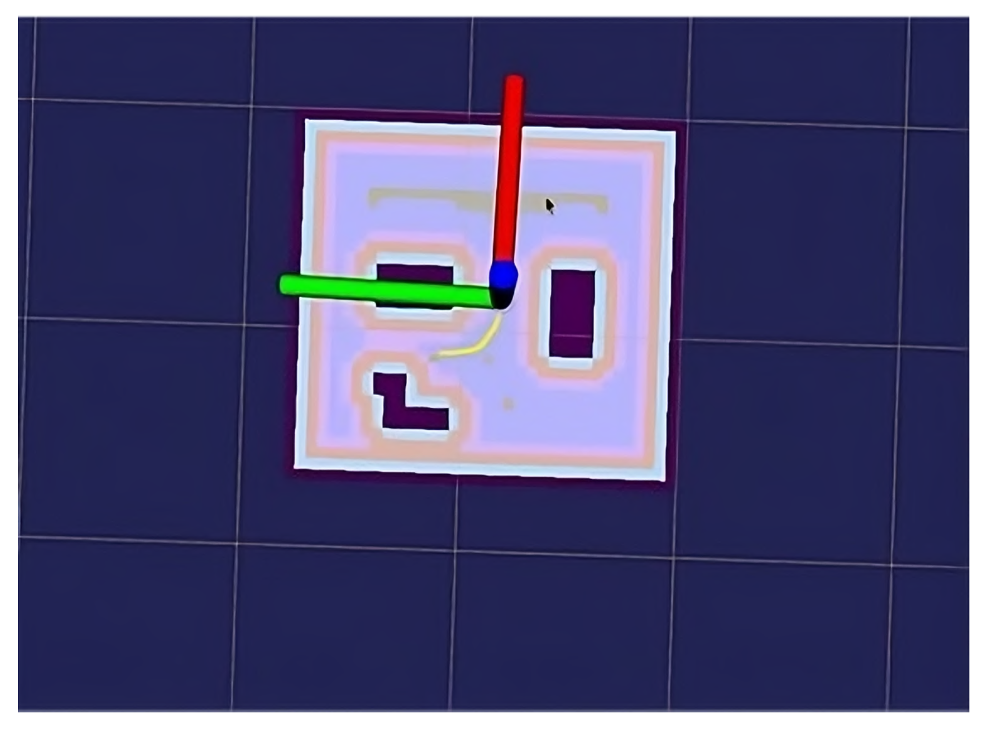
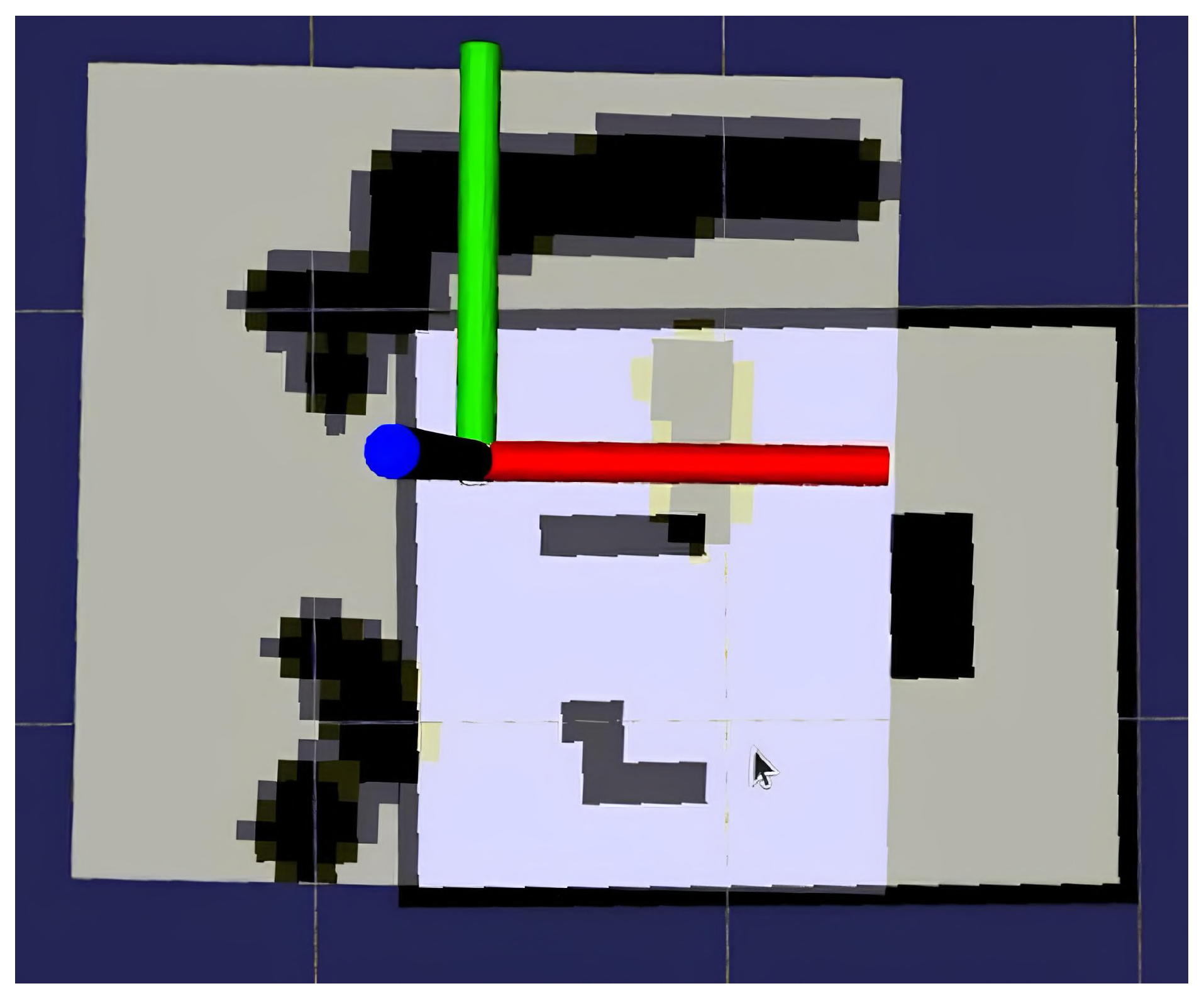
Figure 12 is a view from the ROS Rviz interface of the map used for tests. It is a square of 1.2 m2 with three fixed rectangular obstacles. The rest of the map is available to navigate through. A 0.15 m safety distance is necessary between the robot and the obstacles. This is due to two reasons: to bridge the software and the real environment with a measurable tolerance and to prevent the robot from navigating too close to the obstacles. In the same figure, the axis in the middle of the map represents the AMR, where the red axis is oriented in the same way as the X R local axis of the robot (shown in Figure 4), which means that the red segment of the axis points where the ARM is oriented toward.
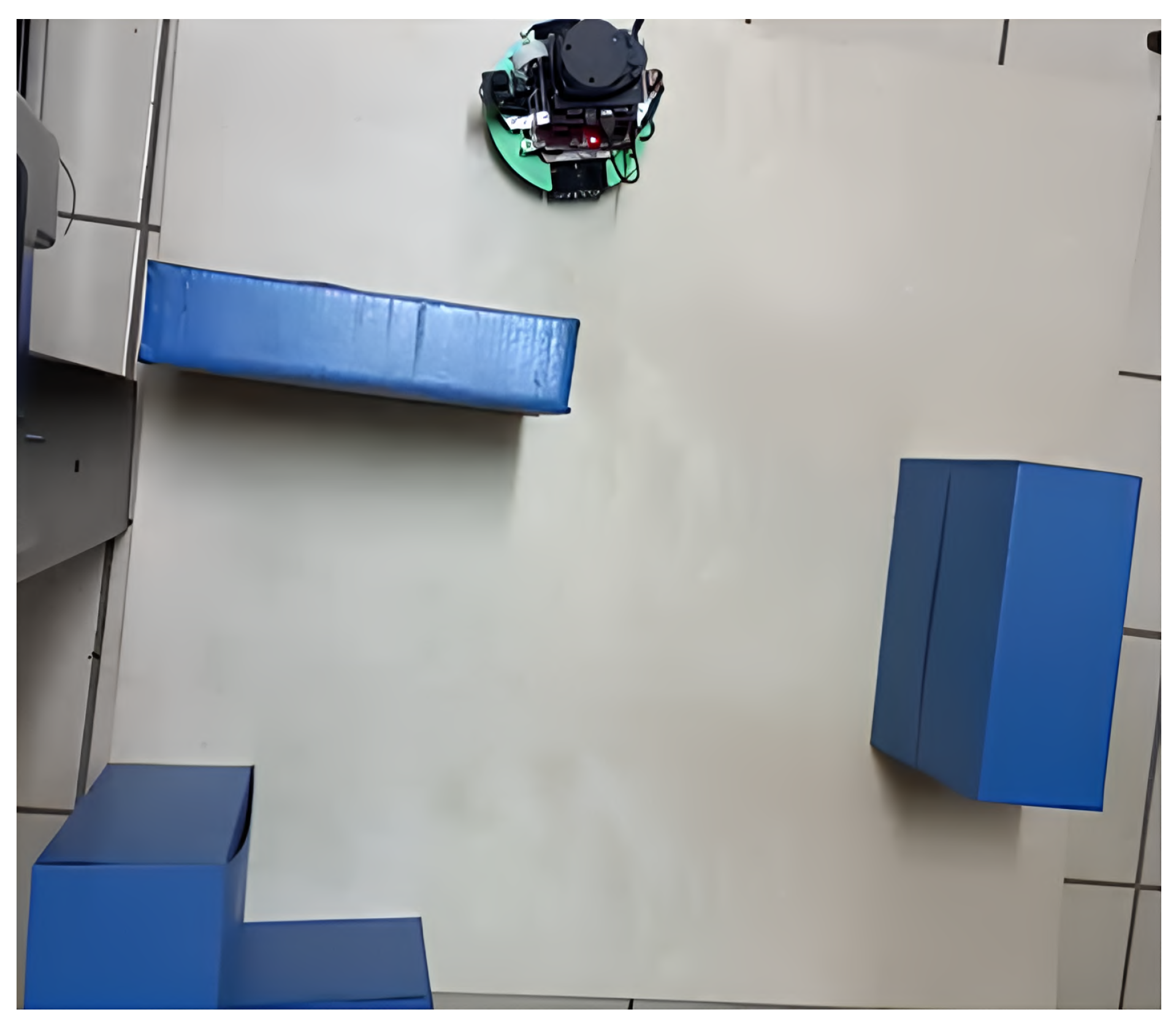
Figure 13 is a photograph of the real environment from Figure 12. The surface is plywood, and its smooth texture helped to prevent the AMR’s wheel system from getting stuck in the floor crevices and indentations, especially during the tuning of the AMR’s linear and angular velocities.
Figure 14 is a local planning map. This helps to notice when a dynamic obstacle approaches the AMR. The map is read through the LiDAR sensor similarly to the mapping process. The figure shows a wall in the upper area that is not considered in the test map. The object in front of the robot (red axis) is a dynamic obstacle, and a person is detected at the bottom of the map.
The laboratory’s mapping is the result of running the LiDAR ROS node provided by Slamtec. It required adjusting settings such as the robot’s initial position and orientation. Then, during the mapping process, the algorithm calculates the robot’s current position based on real-time LiDAR updates.
The result can be saved as a YAML file and a tiff image (Figure 15). The map shows the two-dimensional plane of the environment. The laboratory mapping took approximately 7 min, and the area is nearly 33 m2.
Even though the robot’s velocity was significantly low (0.05 m/s), the angular velocity caused minor errors in the position estimation.
The control of the AMR’s motion results from processing the path planner output signal through a PID controller shown in Figure 7. The need for such control was due to a lack of stability in the path planner output that caused a significant delay while trying to follow the planned route. Said delay also produced unnecessary stops and sometimes the re-planning of the route.
The map has an origin located in the lower left corner. This is the global origin of the map and the odometry system.
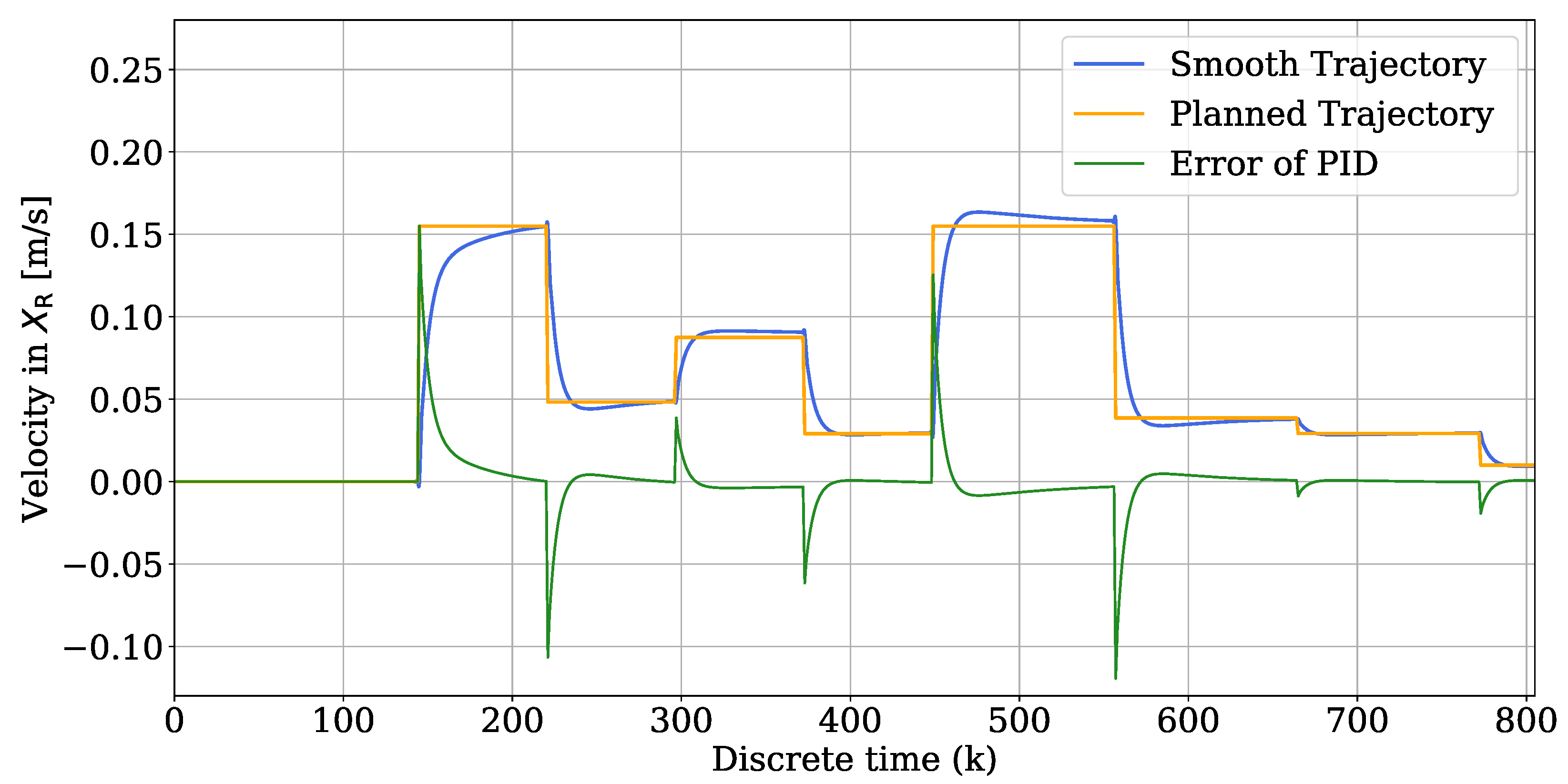
The graph in Figure 16 shows a simulation conducted to visualize the controller’s behavior and fine-tune PID coefficients K p , K i , and K d . The resulting signal (in blue) is smoother and causes a better motion for the AMR-s base control system.
The graphs in Figure 17 and Figure 18 were obtained from a basic motion command of the robot. As Section 3 explains, the map has a global origin shared with the odometry system. This is the global point that the odometry readings of the graphs reference. The behaviors of the signals indicate that the AMR started this particular test at a point 0.6 m from the origin in the X-axis, 0.2 m from the Y-axis, and 0.18 rad from the orientation origin. This corresponds to the one in Figure 5. It moved approximately 0.2 m on the X-axis. And it did not move on the Y-axis. Figure 18 shows the adjustments needed to follow the straight route, approximately an average of 0.05 rad (equivalent to 2 . 8 ).

4.3. Obstacle Detection

The two studied methods were a ResNet18 CNN and YOLOv3 object detector, as described in Section 3; both have different architectures, requirements, and benefits.
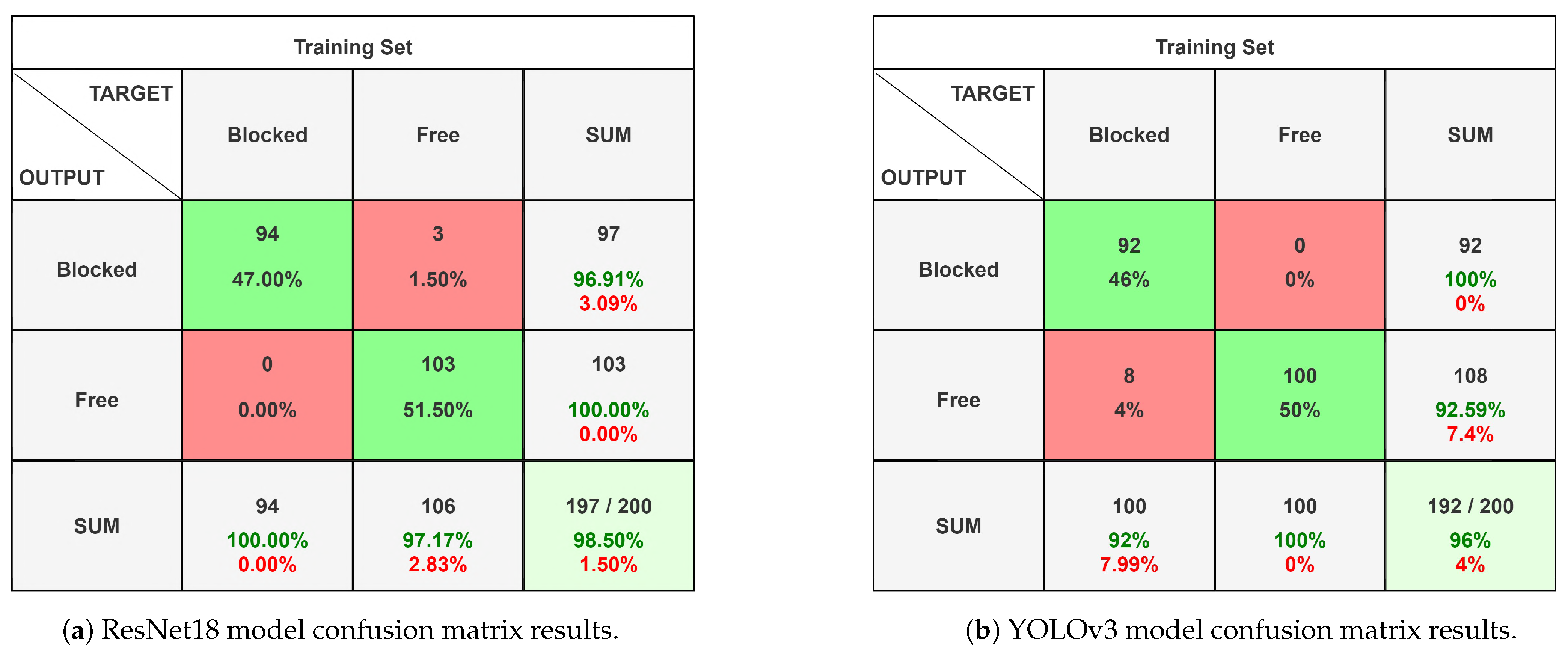
Figure 19 shows the confusion matrices for the CNN artificial vision models. It provides detailed information about the model’s ability to classify the raw images from the robot’s CSI camera into one of the two classes. Figure 19a shows the ResNet18 model’s confusion matrix results, which were, in this case, three false positives for the blocked class and 0 false negatives for the class free.
The second method for object classification was YOLOv3. As mentioned in the Introduction, it has achieved positive results in real-time applications. Moreover, Jetson Nano GPUs enable a DL approach, which helps identify specific objects within the robot’s field of view. This method achieved a similar result as the ResNet18 model, with a difference in that it indicates the location of each obstacle in the scene. As depicted in Figure 19b, the model failed to detect a blocked scene in 8 of 100 attempts.
Table 3 displays the training metrics for the ResNet18 model. The average accuracy was 98.5%, with a precision of 96.91% for the blocked class and 100% for the free class. The recall was 100% for the blocked class and 97.17% for the free class.
Table 4 displays the training metrics for the YOLOv3 model. The average accuracy was 96%, with a precision of 100% for the blocked class and 92.59% for the free class. The recall was 92% for the blocked class and 100% for the free class.
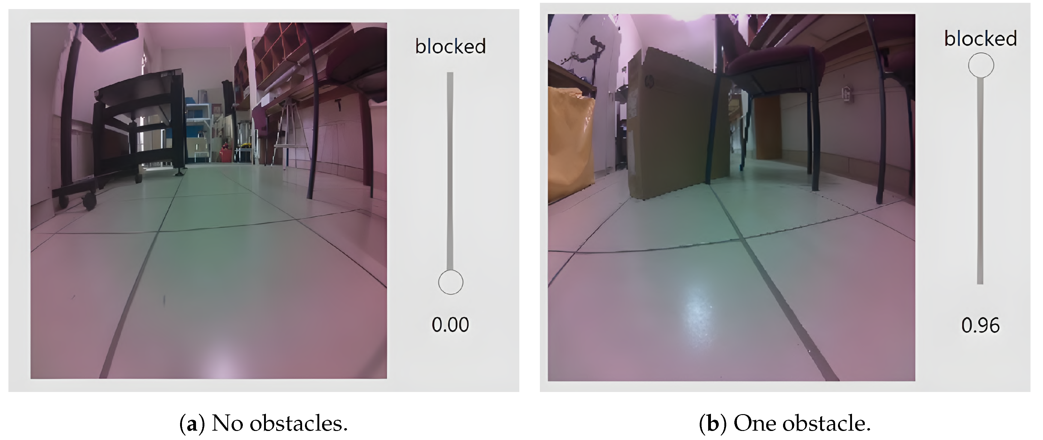
Figure 20 shows two possible situations for the robot’s field of view. In Figure 20a, there are no obstacles in front of the robot, while in Figure 20b, there is a box, being confirmed as an obstacle with an accuracy of 96% by the ResNet18 model. The visual interface used for this experiment was obtained from [50].
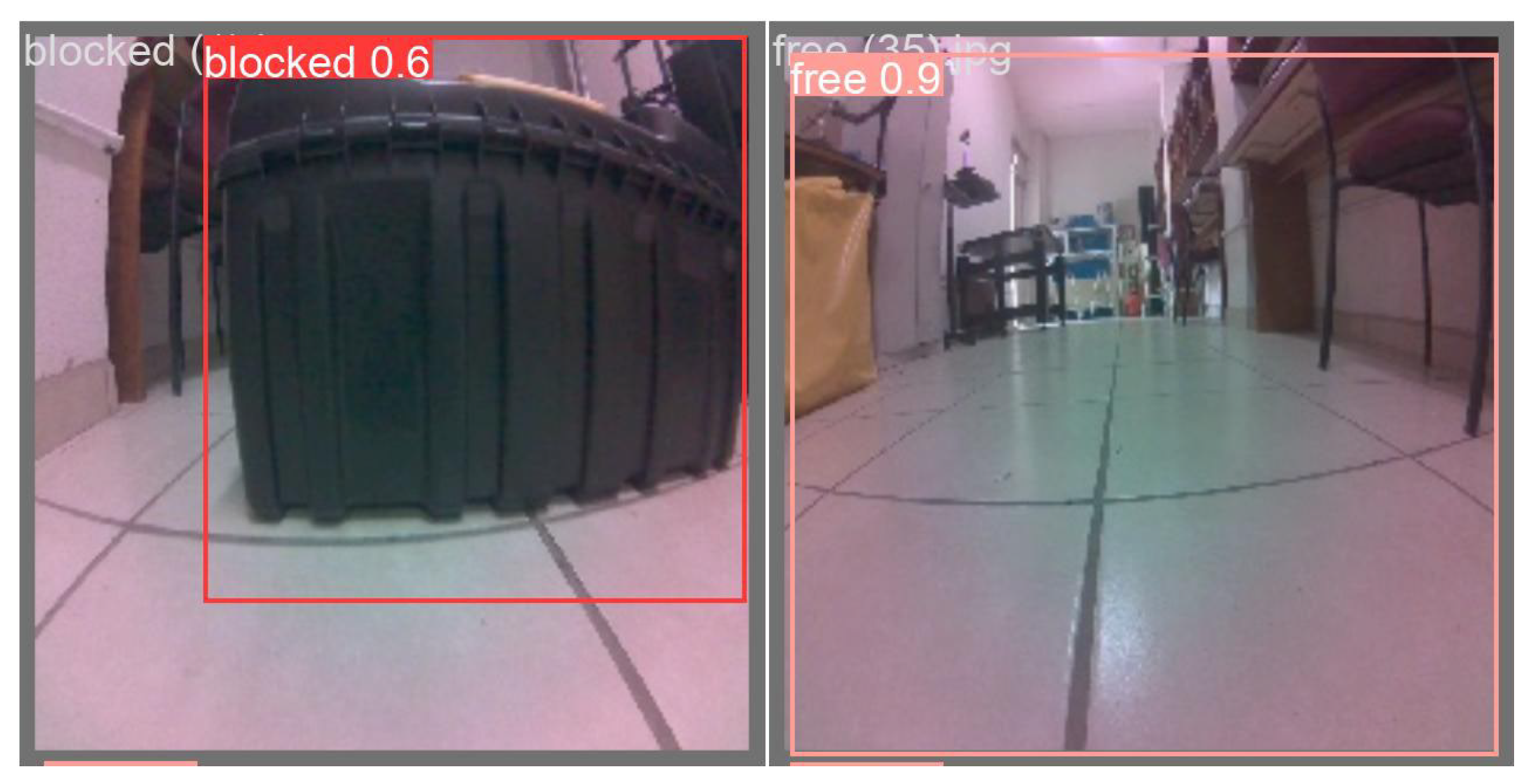
Figure 21 demonstrates the detection process of YOLOv3 for both classes. On the left, it detected an object blocking the path, while on the right, it successfully identified a free area to navigate through. As mentioned, the detector can also interpret the obstacle location and size in the field of view.
We ran a YOLOv3 model pre-trained with the COCO dataset in Jetson Nano as an additional experiment. The resolution used for this experiment was 1280 × 720 pixels, and the model could identify objects accurately with a delay of 5 s. Figure 22 shows the identified classes for that experiment.

5. Discussion

The AMR developed with this methodology incorporates the software tools and DL techniques mentioned earlier in this article. Some of those tools are the operating system ROS, the AMCL algorithm, and object detection with ResNet18 and YOLOv3.
As said, the planning system is subordinate to the AMR’s cognitive abilities; therefore, multiple sensors were added to navigate and read the environment, as seen in Figure 11a. This is the reason why the AMR was constructed the way it is. During the tests, sensors like IMU and LiDAR proved essential to tracking the correct location of the robot on the map. This is also referenced in some of the works included in Table 1; different robots include different sets of sensors depending on the characteristics of the environments and the reliability of said sensor’s data.
The map from Figure 15 used for tests was generated with the mapping tools provided by the ROS mapping package. It helped to compare the data from the sensors easily and consistently. Our experiments in a real environment added extra difficulties compared to the simulated approaches from the literature. However, simulated systems are tools that can provide reliable and useful results quickly.
The graph in Figure 16 indicates the importance of applying additional control to the planned path to achieve a smoother robot motion. This is also referenced in recent investigations [52]. The graphs in Figure 17 and Figure 18 correspond to an improvement compared to the previous performance.
Finally, although the implemented vision system is stable, it is necessary to address the importance of considering using a light version of YOLOv3, which shortens the training process because, ultimately, the vision systems should be capable of detecting obstacles with no need to identify and classify them accurately. In comparing Figure 19a,b, ResNet18 demonstrated a heightened accuracy of 98% in contrast to YOLOv3, which achieved an accuracy of 96%, both trained with the same dataset. Although the overall performances of both CNN models were similar, YOLOv3 detects the exact location of the obstacles in the robot’s field of view.

6. Conclusions

This study presented a methodology for integrating artificial vision, LiDAR localization, and path planning in the low-cost embedded system NVIDIA Jetson Nano. Unlike systems in previous research, the proposed embedded system acted as the central processor, running all the tasks involved in autonomous navigation, including CNN ResNet18 and YOLOv3 training, validation, and real-time execution.
On the other hand, the construction and improvements made to the proposed JetBot AMR required the hardware’s design and the software’s integration. Implementing profound cognitive abilities required the addition of specific devices that helped interpret the robot’s surroundings. The ROS platform provided an environment that enabled the possibility of progressively adding external devices and their functionalities, dividing the project into phases, starting from the most fundamental mechanical characteristics to progressively adding features like sensor fusion and DL algorithms.
Furthermore, the proposed artificial vision system using ResNet18 achieved an average accuracy of 98.5%, a precision of 96.91%, a recall of 97%, and an F1-score of 98.5%. The YOLOv3 CNN achieved an average accuracy of 96%, a precision of 96.2%, a recall of 96%, and an F1-score of 95.99%. Adjusting the settings of YOLOv3 enables multiple possibilities, such as real-time obstacle detection and determining the exact location within the robot camera’s field of view.
After analyzing the results, we confirm that intelligent algorithms are reliable methodologies for solving navigation problems using a heuristic approach.
Finally, according to the description of the hardware used to train RL models in this study, future improvements to such hardware will provide a robust platform for intensive processing using state-of-the-art processors and GPUs, especially in the field of embedded systems.

Future Work

Future work should aim to optimize the object detection system and its communication with the path planner to improve the robot’s overall performance, adding a motion correction routine based on the potential detected obstacles. Moreover, the method described in this work may be reproduced in another mobile robot using the ROS, benefiting from its DL-based vision capabilities. A possible application for the proposed method is as an intelligent robot assistant for the industrial sector.

Author Contributions

Conceptualization, E.E.G.-G. and E.I.-G.; data curation, J.R.C.-V. and C.H.-M.; formal analysis, U.J.T.-P. and O.R.L.-B.; funding acquisition, O.R.L.-B.; investigation, J.G.-F. and S.B.-D.; methodology, J.G.-F. and O.A.A.-C.; project administration, O.R.L.-B.; resources, O.R.L.-B. and E.I.-G.; software, J.G.-F. and O.A.A.-C.; supervision, E.E.G.-G. and E.I.-G.; validation, E.E.G.-G., S.B.-D. and J.R.C.-V.; visualization, U.J.T.-P. and C.H.-M.; writing—original draft, J.G.-F. and O.A.A.-C.; writing—review and editing, E.I.-G. and E.E.G.-G. All authors have read and agreed to the published version of the manuscript.

Funding

This research was funded by the Autonomous University of Baja California (UABC) through the 22nd internal call with grant number 679. The authors also want to thank CONAHCyT for the scholarship awarded to J. Galarza-Falfan for his postgraduate studies with CVU number 1199685.

Institutional Review Board Statement

Not applicable.

Informed Consent Statement

Not applicable.

Data Availability Statement

Data will be available upon request.

Conflicts of Interest

The authors declare no conflicts of interest.

Abbreviations

The following abbreviations are used in this manuscript:
AMRAutonomous Mobile Robot;
ANNArtificial Neural Network;
CNNConvolutional Neural Network;
CPUCentral Processing Unit;
DCDirect Current;
DLDeep Learning;
GPUGraphics Processing Unit;
IMUInertial Measurement Unit;
LiDARLight Detection and Ranging;
MLMachine Learning;
PIDProportional Integral Derivative;
RLReinforcement Learning;
ROSRobot Operating System;
SLAMSimultaneous Localization and Mapping;
UPSUninterruptible Power Supply;
YOLOv3You Only Look Once version 3;
I2CInter-Integrated Circuit;
NASANational Aeronautics and Space Administration.

References

  1. Das, S.; Mishra, S.K. A Machine Learning approach for collision avoidance and path planning of mobile robot under dense and cluttered environments. Comput. Electr. Eng. 2022, 103, 108376. [Google Scholar] [CrossRef]
  2. Cui, J.; Nie, G. Motion Route Planning and Obstacle Avoidance Method for Mobile Robot Based on Deep Learning. J. Electr. Comput. Eng. 2022, 2022, 5739765. [Google Scholar] [CrossRef]
  3. Kheirandish, M.; Yazdi, E.A.; Mohammadi, H.; Mohammadi, M. A fault-tolerant sensor fusion in mobile robots using multiple model Kalman filters. Robot. Auton. Syst. 2023, 161, 104343. [Google Scholar] [CrossRef]
  4. Ishihara, Y.; Takahashi, M. Empirical study of future image prediction for image-based mobile robot navigation. Robot. Auton. Syst. 2022, 150, 104018. [Google Scholar] [CrossRef]
  5. Injarapu, A.S.H.H.; Gawre, S.K. A Survey of Autonomous Mobile Robot Path Planning Approaches. In Proceedings of the International Conference on Recent Innovations in Signal Processing and Embedded Systems (RISE), Bhopal, India, 27–29 October 2017; pp. 624–628. [Google Scholar] [CrossRef]
  6. Zafar, M.N.; Mohanta, J.C. Methodology for Path Planning and Optimization of Mobile Robots: A Review. Procedia Comput. Sci. 2018, 133, 141–152. [Google Scholar] [CrossRef]
  7. Keirsey, D.; Koch, E.; McKisson, J.; Meystel, A.; Mitchell, J. Algorithm of navigation for a mobile robot. In Proceedings of the 1984 IEEE International Conference on Robotics and Automation, Atlanta, GA, USA, 13–15 March 1984; Volume 1, pp. 574–583. [Google Scholar] [CrossRef]
  8. Nilsson, N.J. A mobile automation: An application of artificial intelligence techniques. In Proceedings of the 1st International Joint Conference on Artificial Intelligence (IJCAI-69), Washington, DC, USA, 7–9 May 1969; pp. 509–520. [Google Scholar]
  9. Miller, J.A. Autonomous Guidance and Control of a Roving Robot; Guidance and Control Section; Jet Propulsion Laboratory Pasadena: Pasadena, CA, USA, 1977. [Google Scholar]
  10. Auh, E.; Kim, J.; Joo, Y.; Park, J.; Lee, G.; Oh, I.; Pico, N.; Moon, H. Unloading sequence planning for autonomous robotic container-unloading system using A-star search algorithm. Eng. Sci. Technol. Int. J. 2024, 50, 101610. [Google Scholar] [CrossRef]
  11. Yang, L.; Bi, J.; Yuan, H. Dynamic Path Planning for Mobile Robots with Deep Reinforcement Learning. IFAC-PapersOnLine 2022, 55, 19–24. [Google Scholar] [CrossRef]
  12. Zhang, L.; Cai, Z.; Yan, Y.; Yang, C.; Hu, Y. Multi-agent policy learning-based path planning for autonomous mobile robots. Eng. Appl. Artif. Intell. 2024, 129, 107631. [Google Scholar] [CrossRef]
  13. Kiran, B.R.; Sobh, I.; Talpaert, V.; Mannion, P.; Sallab, A.A.A.; Yogamani, S.; Pérez, P. Deep Reinforcement Learning for Autonomous Driving: A Survey. IEEE Trans. Intell. Transp. Syst. 2022, 23, 4909–4926. [Google Scholar] [CrossRef]
  14. Wang, Y.; Lu, C.; Wu, P.; Zhang, X. Path planning for unmanned surface vehicle based on improved Q-Learning algorithm. Ocean Eng. 2024, 292, 116510. [Google Scholar] [CrossRef]
  15. Zhou, Q.; Lian, Y.; Wu, J.; Zhu, M.; Wang, H.; Cao, J. An optimized Q-Learning algorithm for mobile robot local path planning. Knowl.-Based Syst. 2024, 286, 111400. [Google Scholar] [CrossRef]
  16. Qin, H.; Shao, S.; Wang, T.; Yu, X.; Jiang, Y.; Cao, Z. Review of Autonomous Path Planning Algorithms for Mobile Robots. Drones 2023, 7, 211. [Google Scholar] [CrossRef]
  17. Singh, R.; Ren, J.; Lin, X. A Review of Deep Reinforcement Learning Algorithms for Mobile Robot Path Planning. Vehicles 2023, 5, 1423–1451. [Google Scholar] [CrossRef]
  18. Kou, X.; Liu, S.; Cheng, K.; Qian, Y. Development of a YOLO-V3-based model for detecting defects on steel strip surface. Measurement 2021, 182, 109454. [Google Scholar] [CrossRef]
  19. Redmon, J.; Farhadi, A. YOLOv3: An Incremental Improvement. arXiv 2018, arXiv:1804.02767. [Google Scholar] [CrossRef]
  20. de Carvalho, K.B.; Batista, H.B.; Oliveira, I.L.D.; Brandao, A.S. A 3D Q-Learning Algorithm for Offline UAV Path Planning with Priority Shifting Rewards. In Proceedings of the 2022 19th Latin American Robotics Symposium, 2022 14th Brazilian Symposium on Robotics and 2022 13th Workshop on Robotics in Education, LARS-SBR-WRE 2022, São Bernardo do Campo, Brazil, 18–19 October 2022; pp. 169–174. [Google Scholar] [CrossRef]
  21. Zheng, X.; Wu, Y.; Zhang, L.; Tang, M.; Zhu, F. Priority-aware path planning and user scheduling for UAV-mounted MEC networks: A deep reinforcement learning approach. Phys. Commun. 2024, 62, 102234. [Google Scholar] [CrossRef]
  22. Albonico, M.; Dordevic, M.; Hamer, E.; Malavolta, I. Software engineering research on the Robot Operating System: A systematic mapping study. J. Syst. Softw. 2023, 197, 111574. [Google Scholar] [CrossRef]
  23. Macenski, S.; Foote, T.; Gerkey, B.; Lalancette, C.; Woodall, W. Robot Operating System 2: Design, architecture, and uses in the wild. Sci. Robot. 2022, 7, eabm6074. [Google Scholar] [CrossRef]
  24. Piyapunsutti, S.; Guzman, E.L.D.; Chaichaowarat, R. Navigating Mobile Manipulator Robot for Restaurant Application Using Open-Source Software. In Proceedings of the 2023 IEEE International Conference on Robotics and Biomimetics (ROBIO), Koh Samui, Thailand, 4–9 December 2023. [Google Scholar] [CrossRef]
  25. Huang, B.; Xie, J.; Yan, J. Inspection Robot Navigation Based on Improved TD3 Algorithm. Sensors 2024, 24, 2525. [Google Scholar] [CrossRef]
  26. Estefo, P.; Simmonds, J.; Robbes, R.; Fabry, J. The Robot Operating System: Package reuse and community dynamics. J. Syst. Softw. 2019, 151, 226–242. [Google Scholar] [CrossRef]
  27. Lamini, C.; Fathi, Y.; Benhlima, S. H-MAS architecture and reinforcement learning method for autonomous robot path planning. In Proceedings of the 2017 Intelligent Systems and Computer Vision (ISCV), Fez, Morocco, 17–19 April 2017; pp. 1–7. [Google Scholar] [CrossRef]
  28. Ruan, X.; Lin, C.; Huang, J.; Li, Y. Obstacle avoidance navigation method for robot based on deep reinforcement learning. In Proceedings of the 2022 IEEE 6th Information Technology and Mechatronics Engineering Conference (ITOEC), Chongqing, China, 4–6 March 2022; Volume 6, pp. 1633–1637. [Google Scholar] [CrossRef]
  29. Han, H.; Wang, J.; Kuang, L.; Han, X.; Xue, H. Improved Robot Path Planning Method Based on Deep Reinforcement Learning. Sensors 2023, 23, 5622. [Google Scholar] [CrossRef] [PubMed]
  30. Chen, Y.; Liang, L. SLP-Improved DDPG Path-Planning Algorithm for Mobile Robot in Large-Scale Dynamic Environment. Sensors 2023, 23, 3521. [Google Scholar] [CrossRef] [PubMed]
  31. del R. Millán, J. Reinforcement learning of goal-directed obstacle-avoiding reaction strategies in an autonomous mobile robot. Robot. Auton. Syst. 1995, 15, 275–299. [Google Scholar] [CrossRef]
  32. VOSviewer. Available online: https://www.vosviewer.com/ (accessed on 1 June 2023).
  33. Kastner, L.; Bhuiyan, T.; Le, T.A.; Treis, E.; Cox, J.; Meinardus, B.; Kmiecik, J.; Carstens, R.; Pichel, D.; Fatloun, B.; et al. Arena-Bench: A Benchmarking Suite for Obstacle Avoidance Approaches in Highly Dynamic Environments. IEEE Robot. Autom. Lett. 2022, 7, 9477–9484. [Google Scholar] [CrossRef]
  34. Wang, B.; Liu, Z.; Li, Q.; Prorok, A. Mobile robot path planning in dynamic environments through globally guided reinforcement learning. IEEE Robot. Autom. Lett. 2020, 5, 6932–6939. [Google Scholar] [CrossRef]
  35. Park, M.; Ladosz, P.; Oh, H. Source Term Estimation Using Deep Reinforcement Learning with Gaussian Mixture Model Feature Extraction for Mobile Sensors. IEEE Robot. Autom. Lett. 2022, 7, 8323–8330. [Google Scholar] [CrossRef]
  36. Zheng, Z.; Cao, C.; Pan, J. A Hierarchical Approach for Mobile Robot Exploration in Pedestrian Crowd. IEEE Robot. Autom. Lett. 2022, 7, 175–182. [Google Scholar] [CrossRef]
  37. Chen, Y.; Rosolia, U.; Ubellacker, W.; Csomay-Shanklin, N.; Ames, A. Interactive Multi-Modal Motion Planning with Branch Model Predictive Control. IEEE Robot. Autom. Lett. 2022, 7, 5365–5372. [Google Scholar] [CrossRef]
  38. Yin, Y.; Chen, Z.; Liu, G.; Guo, J. A Mapless Local Path Planning Approach Using Deep Reinforcement Learning Framework. Sensors 2023, 23, 2036. [Google Scholar] [CrossRef]
  39. Park, M.; Lee, S.; Hong, J.; Kwon, N. Deep Deterministic Policy Gradient-Based Autonomous Driving for Mobile Robots in Sparse Reward Environments. Sensors 2022, 22, 9574. [Google Scholar] [CrossRef]
  40. Kozjek, D.; Malus, A.; Vrabič, R. Reinforcement-learning-based route generation for heavy-traffic autonomous mobile robot systems. Sensors 2021, 21, 4809. [Google Scholar] [CrossRef] [PubMed]
  41. Pei, M.; An, H.; Liu, B.; Wang, C. An Improved Dyna-Q Algorithm for Mobile Robot Path Planning in Unknown Dynamic Environment. IEEE Trans. Syst. Man Cybern. Syst. 2022, 52, 4415–4425. [Google Scholar] [CrossRef]
  42. Sivaranjani, A.; Vinod, B. Artificial Potential Field Incorporated Deep-Q-Network Algorithm for Mobile Robot Path Prediction. Intell. Autom. Soft Comput. 2023, 35, 1135–1150. [Google Scholar] [CrossRef]
  43. Wang, X.; Liu, J.; Nugent, C.; Cleland, I.; Xu, Y. Mobile agent path planning under uncertain environment using reinforcement learning and probabilistic model checking. Knowl.-Based Syst. 2023, 264, 110355. [Google Scholar] [CrossRef]
  44. Yeom, K. Collision avoidance for a car-like mobile robots using deep reinforcement learning. Int. J. Emerg. Technol. Adv. Eng. 2021, 11, 22–30. [Google Scholar] [CrossRef] [PubMed]
  45. Hu, J.; Niu, H.; Carrasco, J.; Lennox, B.; Arvin, F. Voronoi-Based Multi-Robot Autonomous Exploration in Unknown Environments via Deep Reinforcement Learning. IEEE Trans. Veh. Technol. 2020, 69, 14413–14423. [Google Scholar] [CrossRef]
  46. Xiang, J.; Li, Q.; Dong, X.; Ren, Z. Continuous Control with Deep Reinforcement Learning for Mobile Robot Navigation. In Proceedings of the 2019 Chinese Automation Congress, CAC, Hangzhou, China, 22–24 November 2019; pp. 1501–1506. [Google Scholar] [CrossRef]
  47. Vohra, D.; Garg, P.; Ghosh, S. Power Management of Drones. Lect. Notes Civ. Eng. 2023, 304, 555–569. [Google Scholar] [CrossRef] [PubMed]
  48. Scaramuzza, D.; Siegwart, R.; Nourbakhsh, I.R. Introduction to Autonomous Mobile Robots, 2nd ed.; MIT Press: Cambridge, MA, USA, 2011. [Google Scholar]
  49. He, S.; Song, T.; Wang, P.; Ding, C.; Wu, X. An Enhanced Adaptive Monte Carlo Localization for Service Robots in Dynamic and Featureless Environments. J. Intell. Robot. Syst. 2023, 108, 6. [Google Scholar] [CrossRef]
  50. Automatic Obstacle Avoiding—Waveshare Wiki. Available online: https://www.waveshare.com/wiki/Automatic_Obstacle_Avoiding (accessed on 15 January 2023).
  51. He, K.; Zhang, X.; Ren, S.; Sun, J. Deep Residual Learning for Image Recognition. In Proceedings of the 2016 IEEE Conference on Computer Vision and Pattern Recognition (CVPR 2016), Las Vegas, NV, USA, 27–30 June 2016. [Google Scholar] [CrossRef]
  52. Gao, H.; Zhou, R.; Tomizuka, M.; Xu, Z. Online Learning Based Mobile Robot Controller Adaptation for Slip Reduction. IFAC-PapersOnLine 2023, 56, 1301–1306. [Google Scholar] [CrossRef]
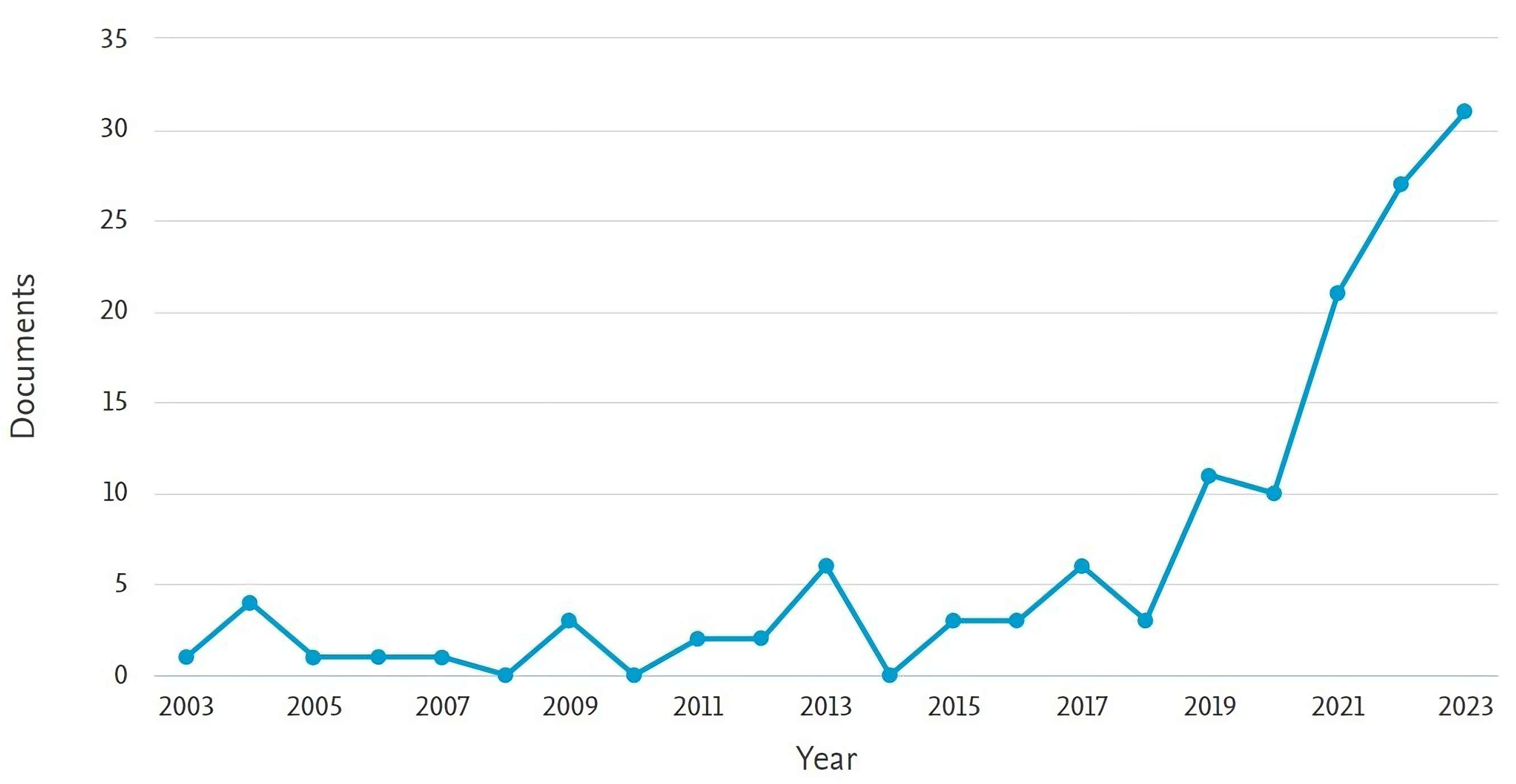
Figure 1. Tendency of the publication of documents found on Scopus by year based on the following keywords: Path Planning AND Autonomous Mobile Robot AND Reinforcement Learning.
Technologies 12 00082 g001
Figure 2. VOSviewer map of the connections between the 40 most relevant keywords found on the database acquired from Scopus.
Technologies 12 00082 g002
Figure 3. Block diagram of the proposed AMR and its remote communication. Note: White arrows represent ROS communications. Black arrows represent other types of communications like I2C or digital I/O.
Technologies 12 00082 g003
Figure 4. Graphic representation of the global and local coordinate systems.
Technologies 12 00082 g004
Figure 5. Graphic representation of the robot’s cinematic model.
Technologies 12 00082 g005
Figure 7. Control used to adjust the output velocity signal based on the AMR’s interaction with the environment.
Technologies 12 00082 g007
Figure 8. ROS nodes (ovals) and their respective topics (rectangles).
Technologies 12 00082 g008
Figure 9. Structure of YOLOv3, also referred to as Darknet-53, taken from [19].
Technologies 12 00082 g009
Figure 11. Robot in its environment.
Technologies 12 00082 g011
Figure 12. Map used for tests seen through Rviz. Red is the X R -axis, green is the Y R -axis, blue is the Z R -axis, the yellow curve is the planned path, the cyan space is the map area where the robot can move, the purple objects are the obstacles, and the pink is the boundary around the obstacles.
Technologies 12 00082 g012
Figure 13. Real environment for the robot to navigate through during tests.
Technologies 12 00082 g013
Figure 14. Local map that contains the dynamic obstacles. Red is the X R -axis, green is the Y R -axis, blue is the Z R -axis, the cyan area in the map is LiDAR-detected free space, black is the dynamic obstacles, and the grey is the detection area of LiDAR.
Technologies 12 00082 g014
Figure 15. Map created using Hector SLAM algorithm. The dark blue is the boundary of the map and fixed obstacles, the purple curve indicates the tracked path of the robot during the mapping process, and the yellow arrow is the final position and orientation of the robot.
Technologies 12 00082 g015
Figure 16. Command velocity read during the movement of the AMR (yellow), the PID-controlled signal (blue), and the controller error (green).
Technologies 12 00082 g016
Figure 17. Odometry readings of X-axis (blue) and Y-axis (orange) during the AMR’s movement.
Technologies 12 00082 g017
Figure 18. Odometry orientation reading from ROS during the AMR’s movement. The blue curve represents the adjustment of the odometry.
Technologies 12 00082 g018
Figure 19. Confusion matrices show the correctly identified classes in green and the incorrect ones in red for the CNN artificial vision models.
Technologies 12 00082 g019
Figure 20. Robot’s field of view with the two possible classes.
Technologies 12 00082 g020
Figure 21. Predictions of the YOLOv3 model for both classes. Red square represents a blocked path, and pink square represents a free path.
Technologies 12 00082 g021
Figure 22. Pre-trained YOLOv3 model, capable of detecting up to 80 classes.
Technologies 12 00082 g022
Table 1. Brief descriptions of the hardware used in different experiments of RL algorithms and models.
ReferenceAlgorithm/ModelHardwareResultsYear
This workResNet18 and YOLOv3 running on ROS MelodicNVIDIA Jetson NANO, MPCore processor Quad-core, 128-core Maxwell 1098 MHz, 4 GB DDR4 RAMThe vision system prevents collisions with dynamic obstacles, reaching an accuracy of 98.5%, a recall of 97%, and an F1-score of 98.5%2024
Wang et al. [43]QEA-LearningIntel(R) Core(TM) i5-7200 CPU, with 2.50 GHz and 2.71 GHzThe QEA-Learning algorithm reduces the probability of failure by assigning less weight to the reward function2023
Yang et al. [11]DRL, Soft Actor-Critic (SAC), Pro-
ximal Policy Optimization (PPO)
Intel Xeron(R) CPU E5-2650 v4 at 2.20 GHzSAC performed better than PPO by finding a higher maximum reward and better exploration–exploitation balance2022
Ruan et al. [28]DRL, Dobule Q-Network (D3QN)NVIDIA GTX 3080 GPU, Robot Operating System (ROS)The loss function stabilizes after 1000 training trials2022
De Carvalho et al. [20]Q-Learning16 GB of RAM, Intel Core i7-7700Processing time under 2 min for 20 × 20 × 5 cell maps2022
Yeom [44]DRLRaspberry Pi 3, Quad Core 1.2 GHz, Intel 4-core i5 7500 CPU, 3.80 GHz, 32 GB RAMDRL reduced path length by approximately 20% compared to the traditional Dynamic Window Approach (DWA)2021
Hu et al. [45]Deep Deterministic Policy Gradient (DDPG), Prioritized Experience Replay (PER)Raspberry Pi 3, NVIDIA GTX 1080 GPU, Intel Core i9 CPU with 2.9 GHzThe algorithm performed 20 successful missions and required 40 min of training time2020
Xiang et al. [46]DRL, Soft Actor-Critic (SAC)NVIDIA GeForce RTX 2070 GPU, 3.70 GHz eight-core AMD Ryzen 7 2700X, 16 GB RAM, ROSThe model was compared against traditional gmapping navigation, reaching competitive results after hours of training2019
Table 2. Training hyperparameters for ResNet18 model.
ParameterValue
OptimizerSDG
Learning rate0.001
Momentum0.9
Epochs10
Batch size8
Table 3. ResNet18 CNN training metrics.
Class NamePrecision1-PrecisionRecall1-RecallF1-Score
Blocked0.96910.03091.00000.00000.9843
Free1.00000.00000.97170.02830.9856
Accuracy0.9850
Misclassification Rate0.0150
Macro-F10.9850
Weighted-F10.9850
Table 4. YOLOv3 CNN training metrics.
Class NamePrecision1-PrecisionRecall1-RecallF1-Score
Blocked100.920.07990.9583
Free0.92590.074100.9615
Accuracy0.96
Misclassification Rate0.04
Macro-F10.9599
Weighted-F10.9599
Disclaimer/Publisher’s Note: The statements, opinions and data contained in all publications are solely those of the individual author(s) and contributor(s) and not of MDPI and/or the editor(s). MDPI and/or the editor(s) disclaim responsibility for any injury to people or property resulting from any ideas, methods, instructions or products referred to in the content.