Particle Movement in DEM Models and Artificial Neural Network for Validation by Using Contrast Points

Abstract

The calibration and validation of input parameters in the Discrete Element Method (DEM) are crucial for accurately simulating physical processes, typically achieved through experimental particle behavior analysis. Enhancing the accuracy of DEM models allows for more reliable predictions of material behavior, which is essential for optimizing engineering applications that involve particulate materials. In this study, we present a methodology for analyzing the movement properties of particulate materials, employing a combination of Caliscope software to obtain the real-world co-ordinates based on pixel values from both cameras and artificial neural networks for regression as straightforward and efficient tools. This approach enables the validation and calibration of digital twins of particulate matter systems with respect to motion characteristics. The method of contrast points was utilized to acquire spatial co-ordinates of particulate material movement from experimental measurements, facilitating precise trajectory determination and the subsequent verification of simulation predictions. The neural network analysis demonstrated high accuracy, achieving R² values of 0.9988, 0.9972, and 0.9982 for the X–, Y–, and Z–axes, respectively. The standard deviation between the predicted and actual co-ordinates was found to be 1.8 mm. A comparative analysis of particle trajectories from both the model and experimental data indicated strong agreement, underscoring the soundness and reliability of this approach.

1. Introduction

The agriculture sector continually faces the challenge of optimizing production processes while ensuring sustainability. As the demand for efficient agricultural practices grows, the need for advanced modeling techniques has become increasingly apparent. The Discrete Element Method (DEM), introduced by Cundall and Strack in 1979 [1], has emerged as a crucial tool for simulating the behavior of granular materials, making it particularly relevant in agricultural applications [2,3]. DEM allows for the detailed analysis of the movement, interaction, and flow of bulk materials, such as soil, seeds, and fertilizers, providing insights that are essential for enhancing agricultural efficiency and productivity [4,5,6,7].

Before conducting DEM simulations, it is essential to determine the parameters of the DEM model for particulate matter such as the coefficient of restitution, Young’s modulus, the coefficient of friction, and other material properties [8,9,10]. In this process, micromechanical parameters that cannot be directly measured must be adjusted to ensure that the model’s behavior closely resembles that of the real particulate material [11]. One possible approach to parameter calibration is to verify force effects through draft forces [12,13,14]. To determine the draft force, Mouazen et al. (2003) [15] employed a movable instrumented chisel equipped with a soil strength measurement device. This apparatus was used to validate a FEM (Finite Element Method) simulation for estimating the maximum force exerted on the chisel and the dry bulk density. FEM-DEM coupling was utilized in the study by Kešner et al. [16], who focused on stress distribution on a soil tillage machine frame segment with a chisel shank. Kuře et al. [17,18], in his study, verified the agreement of draft forces by employing a DEM model and measurements from an experimental soilbox filled with sand, through which a scaled moveable model of a plowshare with various geometries was driven.

Other possible approach for parameter calibration is through the verification of movement [18]. This can be achieved by testing the angle of repose or by employing passive markers [19]. The use of passive markers involves placing small markers in the soil before pulling a tool through it and subsequently measuring their displacement after the tillage process. This method is cost-effective and suitable for examining different soil layers, however, it is time-consuming and does not provide information on the trajectory of the soil during the measurement [20,21]. These issues can be mitigated through the application of object tracking during the processing of particulate matter on its surface using image analysis [22,23]. In our study [19] in 2022, we traced the movement of rapeseed particles during the discharge process using an experimental device designed to determine the angle of repose. For tracing purposes, contrast points were utilized on the surface of a transparent flow cylinder. This method was effective, however, it used only one camera. Tracking objects with two cameras is more complex and therefore requires more advanced techniques.

Tracing motion using image analysis can be efficiently performed with two cameras, enabling the determination of real-world co-ordinates of specific points in space [24]. This process requires the calculation of both extrinsic and intrinsic parameters of each camera [25,26]. The extrinsic parameters define the camera’s precise position and orientation relative to the world co-ordinate system [27]. In contrast, the intrinsic parameters include the camera’s internal characteristics, such as focal lengths, the principal points, and lens distortion coefficients, that account for lens imperfections that affect image geometry [27,28]. To accurately determine these parameters, a chessboard pattern is commonly used [29]. The chessboard pattern provides multiple reference points for calibration, allowing for the precise extraction of both extrinsic and intrinsic camera properties [30].

Stereoscopic triangulation can be used as an effective technique to determine object trajectories from two cameras. This method allows for the reconstruction of 3D co-ordinates from two 2D camera views by calculating the intersection points of projected lines [27,31]. Various modules in OpenCV provide tools for such stereoscopic vision analysis, enabling extraction of object paths [32]. In addition to traditional computer vision approaches, neural networks can also be utilized to evaluate trajectories [33,34]. Convolutional Neural Networks (CNNs) are capable of automatically learning spatial hierarchies of features, which makes them suitable for object tracking [35]. CNNs enable the identification of patterns such as edges or textures, leading to the detection and classification of objects [36]. For object tracking, Recurrent Neural Networks (RNNs) and Long Short-Term Memory (LSTM) networks are also often used [37]. These models are designed to analyze sequences of frames over time, allowing for the prediction of object movements [37,38].

Neural networks enable the identification of complex nonlinear relationships between input and output variables, such as pixel values from multiple cameras. When well designed and trained, the model can determine spatial points with a certain degree of accuracy. The advantage of this method lies in its ability to directly capture movement trajectories in X, Y, and Z co-ordinates, similar to tracking objects in three-dimensional space [39]. In soil studies, this approach allows for a direct description of the observed particle’s trajectory, enabling a direct comparison with particle movements in the DEM model. This method appears to be more accurate than comparing changes based on the contrast of the entire material with changes in preselected particles within the DEM model [40]. A limitation of this method is that particle movement can only be tracked on the visible surface of the material using a camera. Recent studies are exploring the possibility of tracking particle movement beneath the surface [18,41]. These methods require placing sensor modules, which are significantly larger than the contrast points being tracked. This could potentially affect the flow of the measured material, and this approach requires a rigorous evaluation process [42]. The application of neural networks in conjunction with Discrete Element Method (DEM) models has already been explored. There are numerous studies focusing on the use of neural networks as a tool for predicting the outcomes of DEM models [43,44,45]. For instance, Liao et al. (2021) [46] utilized a convolutional neural network (CNN) to predict the behavior of granular flow in a wedge-shaped silo, reducing the CPU-hours required for DEM simulations under the given conditions.

The aim of this study is to develop a methodology for verifying particle systems modeled using the discrete element method (DEM). The research is conducted in a sand box equipped with two cameras that track the behavior of sand particles during the passage of a tillage tool. A contrast point method is employed to monitor particle motion. Video recordings are subsequently processed, with an artificial neural network (ANN) for regression used as a straightforward and efficient tool for determining X, Y, and Z co-ordinates based on pixel values from both cameras.

A major contribution of this study is that the proposed methodology provides the potential for repeated use of the entire calibration system—both the experimental system and its digital twin—to verify various particulate materials with different properties and compositions. The requirement is to maintain the geometries, positions, and camera settings while changing the particulate substance within the experiment, as well as the input parameters based on the verified particulate system.

2. Materials and Methods

2.1. Camera Calibration-Intrinsic Camera Parameters

Two GoPro Hero 8 Black cameras were used in this study. The GoPro cameras were set to video mode with 4K resolution, 50 FPS and a linear lens. For image analysis, camera calibration was necessary. The calibration was performed using a chessboard pattern, which enabled the determination of the cameras’ focal lengths f_x and f_y, as well as the distortion coefficients. This calibration was conducted separately for each camera and for their combined view.

Videos of the ChArUco chessboard pattern [47] were captured by each camera, and the compressed videos were imported into Caliscope software [48]. This was done to obtain intrinsic parameters of each camera. The original resolution of 2160 × 3840 was reduced to 1080 × 1920, with compression performed in DaVinci Resolve 19 [49]. The size of each square of ChArUco chessboard pattern was 25 mm, with the full grid consisting of eight columns and five rows, measuring 200 × 125 mm. The internal corners of the squares were traced to calculate the intrinsic parameters. This is evident from Figure 1, which is from the side camera’s calibration. In the picture, the inner corners (reference points) are marked in red.

The resulting intrinsic parameters are listed in

Table 1. Intrinsic parameters of GoPro cameras.

Parameter	Side Camera	Front Camera
RMSE	0.463	0.371
Intrinsic parameters
Focal length x (px)	915.81	913.36
Focal length y (px)	919.63	917.34
Optical center x (px)	944.03	944.89
Optical center y (px)	544.69	550.88
Distortion coefficients
Radial k1	−0.0	0.01
Radial k2	0.0	−0.01
Radial k3	−0.0	0.0
Tangential p1	0.0	0.0
Tangential p2	−0.01	−0.01

. For Camera 1, referred to as the side camera, the focal lengths were f_x = 915.81 px and f_y = 919.63 px. For Camera 2, referred to as the front camera, the focal lengths were f_x = 913.36 px and f_y = 917.34 px. The optical center for the side camera was c_x = 944.03 px and c_y = 544.69 px, while for the front camera it was c_x = 944.89 px and c_y = 550.88 px. The distortion coefficients (k₁, k₂, k₃, p₁) for the side camera were near zero, while for the front camera, the radial distortion coefficient k₁ was 0.01 and the radial distortion coefficient was −0.01. The tangential distortion coefficient p₂ was −0.01 for both cameras. The root mean square error (RMSE) was 0.463 for the side camera and 0.371 for the front camera.

2.2. Camera Calibration-Extrinsic Camera Parameters

Consequently, the extrinsic parameters were obtained. The synchronized video recordings were captured using both cameras in the sand box. Figure 2 shows the location of the cameras within the sand box. The side camera is labeled ‘cam 1’ in the image and its location is labeled ‘Location of cam 1’. The front camera is labeled ‘cam 2’ in Figure 2 and its location is labeled ‘Location of cam 2’. The image also highlights the ChArUco chessboard pattern board.

To obtain extrinsic camera parameters, the ChArUco board was used. The view of the board from both perspectives is shown in Figure 3. Figure 3a illustrates the perspective from the side camera, while Figure 3b presents the view from the front camera. The board was moved in various directions and angles to ensure visibility from both cameras. The individual patterns on the board were recognized, and each internal corner was assigned a point number. The board contained 27 points. The variations in the positions of the points under different angles allowed the determination of their 3D spatial positions based on pixel values, while accounting for distortion. The data collected were saved in a *.csv file, which contained pixel values from the side camera (x_s and y_s) and from the front camera (x_f and y_f), as well as the X, Y, and Z co-ordinates of each point at each time step. A total of 44,130 data points were obtained. The world co-ordinate system in [0;0;0] corresponded to the camera co-ordinate system of the side camera.

2.3. Experiment and Equipment Used

The other video recording was captured from both cameras during the passage of a tillage tool through sand containing contrast particles. Due to the previous calibration, the exact positioning of both cameras needed to be maintained throughout the experiment.

The experiment was conducted in a sand box filled with silica sand, dried to 0% moisture content. The particle size of the sand was measured, with the grain fraction ranging from 0.1 to 0.3 mm. The silica sand was poured into the sand box to a height of 240 mm. The dimensions of the sand box were as follows: height 500 mm, width 500 mm, and length 1500 mm. An aluminum model of a tillage tool (chisel), scaled down by a ratio of 1:2 compared to the real tool, was used in the sand box. The tool was equipped with wings, allowing for a broader analysis of its impact on particle movement. The working depth of the tillage tool was set to 75 mm. For the contrast point method, eight wooden contrast particles painted blue were used. These particles measured 5 mm in size and were placed in two rows: one centered along the tool’s path, and the other 50 mm offset from the first. The distance between the individual particles within each row was set at 50 mm. The arrangement of particles on the surface of the sand in the sand box, as viewed from the side camera, is shown in Figure 4. The particles were labeled with numbers 1 to 8.

During the experiment, a winch system was activated to move the tillage tool along the positive Z–axis. The tool’s movement speed was set to 0.1 m·s⁻¹, and it was moved in a total distance of 700 mm. As the tool moved, it passed through the area containing contrast particles, allowing for the observation of the particles’ displacement during the tool’s passage. The entire experiment was recorded by the calibrated cameras, capturing the movement and interactions of the contrast particles in real-time.

2.4. Image Processing with DaVinci Resolve 19

The video recordings were imported into DaVinci Resolve 19 [49]. It was necessary to synchronize the video recordings. This was achieved using audio track synchronization, supplemented by an additional audio marker. Within DaVinci Resolve 19, the Tracker tool was employed, which in this study was used to track the movement of selected points throughout the video. The tracked points were represented by the contrast particles, specifically the wooden spheres. The Tracker tool allowed for the selection of specific areas to be tracked over the course of the video. Figure 5a illustrates a selected contrast particle. For each tracked area, the normalized pixel values on the X– and Y–axes were displayed. These pixel values were normalized to a range from 0 to 1, with the normalized values corresponding to the center of the tracked area. In our study, the values represented the center of the visible clusters of pixels of the contrast particle. The Tracker tool proceeded frame by frame, monitoring the movement of the selected pixel cluster throughout the video. Figure 5b presents the motion paths obtained from the Tracker tool, capturing the movement over 166 frames. The Figure 5b shows the perspective from the side camera. This process needed to be performed also for the perspective from the front camera. The obtained trajectories were then exported into a *.csv file, with the exported data including the motion path and point samples in absolute values. The pixel values on the X– and Y–axes were normalized between 0 and 1. This normalization needed to be considered when converting the traced values back to pixel co-ordinates. For the Y–axis, the normalized data were divided by 0.5625, corresponding to the resolution ratio, which reduced the Y–axis values by this factor. Finally, the values were multiplied by the resolution.

2.5. ANN Development

To obtain real-world co-ordinates from the generated trajectories in DaVinci Resolve 19, based on 3D co-ordinates derived from pixel values, a neural network was developed in Python using the PyCharm development environment. The TensorFlow framework and Keras library were employed to implement a multi-layer perceptron (MLP) model.

The architecture consisted of three hidden layers, each of the Dense type. The first hidden layer had 512 neurons, the second had 1024 neurons, and the third had 256 neurons. The input layer received four inputs derived from two datasets: the first containing pixel values from the side camera (x_s and y_s) and the second containing pixel values from the front camera (x_f and y_f). The activation function used was ReLU (Rectified Linear Unit), and, to prevent overfitting, the Dropout regularization technique was integrated. Both input datasets were normalized to a range between 0 and 1.

The model was trained for 60 epochs with a batch size of 512 and a validation split of 0.2. The output layer predicted three variables: X, Y, and Z co-ordinates in the world co-ordinate system, using a linear activation function. The model was optimized with early stopping to monitor validation errors during training.

The neural network was trained on 44,130 samples generated using Caliscope software, with 40,000 samples designated for training and 4130 for testing. Input values represented x and y pixel co-ordinates from the cameras, while outputs corresponded to spatial positions in X, Y, and Z. The trained model was subsequently used to predict particle trajectories from pixel values obtained in DaVinci Resolve 19, with results exported in a *.csv file. However, before processing, it was necessary to adjust the pixel values from DaVinci Resolve 19, as co-ordinates within this software were calculated from the bottom-left corner, while Caliscope software calculated co-ordinates from the top-left corner.

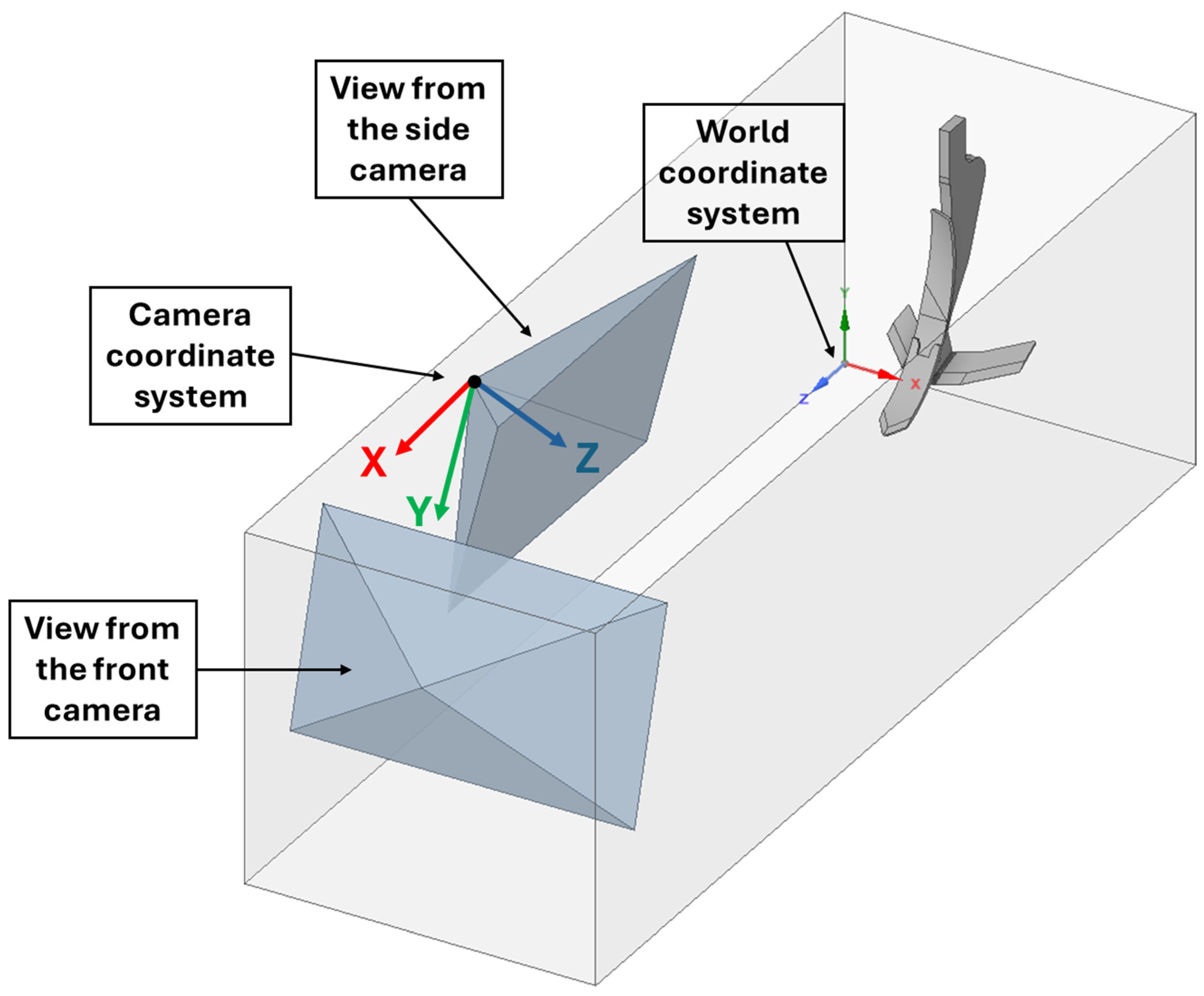
2.6. World Co-Ordinate System Rotation

The ANN was trained on the co-ordinate system from the Caliscope software, which corresponds to the co-ordinate system of the side camera. The co-ordinate system for the predicted values obtained from the neural network based on the pixel values from DaVinci Resolve 19 was directed the same way. The direction of the camera co-ordinate system and the world co-ordinate system within the sand box is shown in Figure 6. The figure also ilustrates the used tillage tool (chisel) presents views from the individual cameras, namely the side camera and the front camera.

Since the original values of the co-ordinate system were symmetrically rotated according to the side camera, it was necessary to transform the global co-ordinate system. The co-ordinate system must have been oriented identically to that of the sand box, meaning that the X–, Y–, and Z–axes must correspond to the walls of the sand box.

The rotation in a 3D system consists of three sequential rotations, each around one axis of the system [50]. The reference plane was established using the plane defined by the points of the calibration plate from the first image, where the plate was oriented in the desired direction. Subsequently, the global co-ordinate system was rotated around the X–axis at the corner point so that the line connecting the extreme points was symmetrical with respect to the Y–axis. Following this, the co-ordinate system was rotated around the Y–axis and then again around the X–axis, ensuring that the orientation of the plane in space matched that of the trough, resulting in a consistent orientation of the co-ordinate system for the evaluated data.

The rotation around the Z–axis is shown in Figure 7.

As can be seen from the figure, the relationship between the co-ordinates of any point A in the original co-ordinate system (x₂, y₂) and the new co-ordinate system (x, y) after rotation by an angle α can be expressed by Equations (1)–(3). This involves rotation around the Z–axis. Similarly, the same approach can be applied for rotation around the other axes. Finally, three successive rotations were used to align the camera co-ordinates with the global co-ordinates.

$$x=x_{2}cos\alpha +y_{2}sin\alpha$$

(1)

$$y={-x}_{2}sin\alpha +y_{2}cos\alpha$$

(2)

$$z=z_2$$

(3)

2.7. Creation of the Digital Twin in Ansys Rocky

The simulation model was developed based on a comprehensive literature review, previous study results, and the validation of the model using the angle of repose and subsequent Design of Experiments (DoE) [17,51,52,53,54,55,56,57,58,59].

2.7.1. The Geometry Creation

The geometry of the sand box was modified from its actual dimensions for simulation purposes. A 3D CAD model was created in Ansys SpaceClaim with dimensions of 510 mm in height, 510 mm in width, and 1200 mm in length, compared to the real box length of 1500 mm. Additionally, the walls were simplified by representing them as surfaces rather than solid walls with thickness. These adjustments significantly reduced the computational time required for the simulation. Furthermore, a model of the tillage tool (chisel) was incorporated. Three-dimensional models were exported and stored in *.stl format. The created geometry in Ansys SpaceClaim is presented in Figure 8. Both models were imported into Ansys Rocky software, where the depth of the tillage tool was set to 75 mm.

2.7.2. The Physics Parameters

Table 2. Gravitational acceleration settings and contact force models.

Physics	Value	Source
Gravity in Y-direction	9.81 m·s−2	-
Normal Force	Hertzian Spring Dashpot	[57]
Tangetial Force	Mindlin-Deresiewicz	[57]
Adhesive Force	None	[57]
Impact Energy	Default	[57]
Rolling Resistance Model	Type C: Linear Spring Rolling Limit	[57]

shows the set gravitation and numerical models. For the normal force model, the Hertzian spring-dashpot model was applied [59]. This model describes nonlinear contact forces and is used for systems involving viscoelastic particle interactions. It combines Hertz’s classical contact theory with damping, providing a more realistic depiction of particle interactions [56,57]. The tangential forces were modeled using the Mindlin-Deresiewicz theory, an extension of elastic contact theory, which describes the frictional interactions between particles. This model is suitable for simulating bulk materials where friction plays a significant role and is used for calculating tangential forces in elastic-friction interactions, where slipping is not considered [57,58]. Adhesion forces were not considered in the model because the simulated silica sand was dry, and adhesion under such conditions was assumed to be negligible. This assumption aligns with previous studies, which have shown that at zero moisture content, adhesion between sand particles is minimal [8]. For rolling resistance, a linear spring rolling limit model was used, which is commonly applied to simulate particle rotation during motion. Gravitational acceleration was set along the Y–axis with a value of −9.81 m·s⁻².

2.7.3. Materials Settings

The materials used in the simulation were defined, including the materials for the surrounding geometry and the particles (

Table 3. Material settings for the surrounding geometry and for the particles.

Material Settings	Value	Source
Particles
Bulk Density	1533 kg·m−3	[17]
Young’s Modulus	1.7 MPa	[17]
Poisson’s ratio	DoE	[51,52]
Boundary
Density	7850 kg·m−3	[17]
Young’s Modulus	1 × 1011 N·m−2	[17]
Poisson’s ratio	0.3	default

). The bulk density and Young’s modulus were determined based on previous research. Poisson’s ratio for the aluminum tool was set as the default and the sand was sourced from a literature review [51,52] and was subsequently one of the objects of the DoE process.

2.7.4. The Material Interactions

The interactions between particles, as well as between particles and geometry, were also defined. The interaction settings are summarized in

Table 4. Material settings of interactions between particles and particles and between surrounding geometry and particles.

Materials Interactions	Value	Source
Particles × Particles
Static Friction	0.71	[17]
Dynamic Friction	0.59	[17]
Restitution Coefficient	DoE	-
Particles × Boundary
Static Friction	0.4	[17]
Dynamic Friction	0.3	[17]
Restitution Coefficient	0.3	default

. The static and dynamic friction values for these interactions were determined experimentally based on previous research [17,53]. The restitution coefficient was refined through the DoE process.

2.7.5. Particle Setting

Subsequently, the particle parameters were defined, with their sizes increased for simplification of the model. The simulation used a single type of spherical particles, differentiated into two sizes. These particles were organized into two layers (the particle inlets) based on their size. The lower layer, which did not directly interact with the agricultural tool, consisted of larger particles with a diameter of 10 mm. The upper layer, in direct contact with the tillage tool, contained particles with a diameter of 2 mm. This distinction in particle sizes was implemented to simplify the simulation and reduce computational demands while maintaining accuracy in areas where interactions with the tillage tool were expected. In the simulation, rolling resistance was enabled, and its value was determined through a DoE process. The specific parameter settings are provided in

Table 5. Particle parameter settings.

Particles Settings		Source
Shape	Sphere	-
Material	Default Particles	-
Size
Particle 1	2 mm	-
Particle 2	10 mm	-
Rolling Resistance	DoE	[17]

.

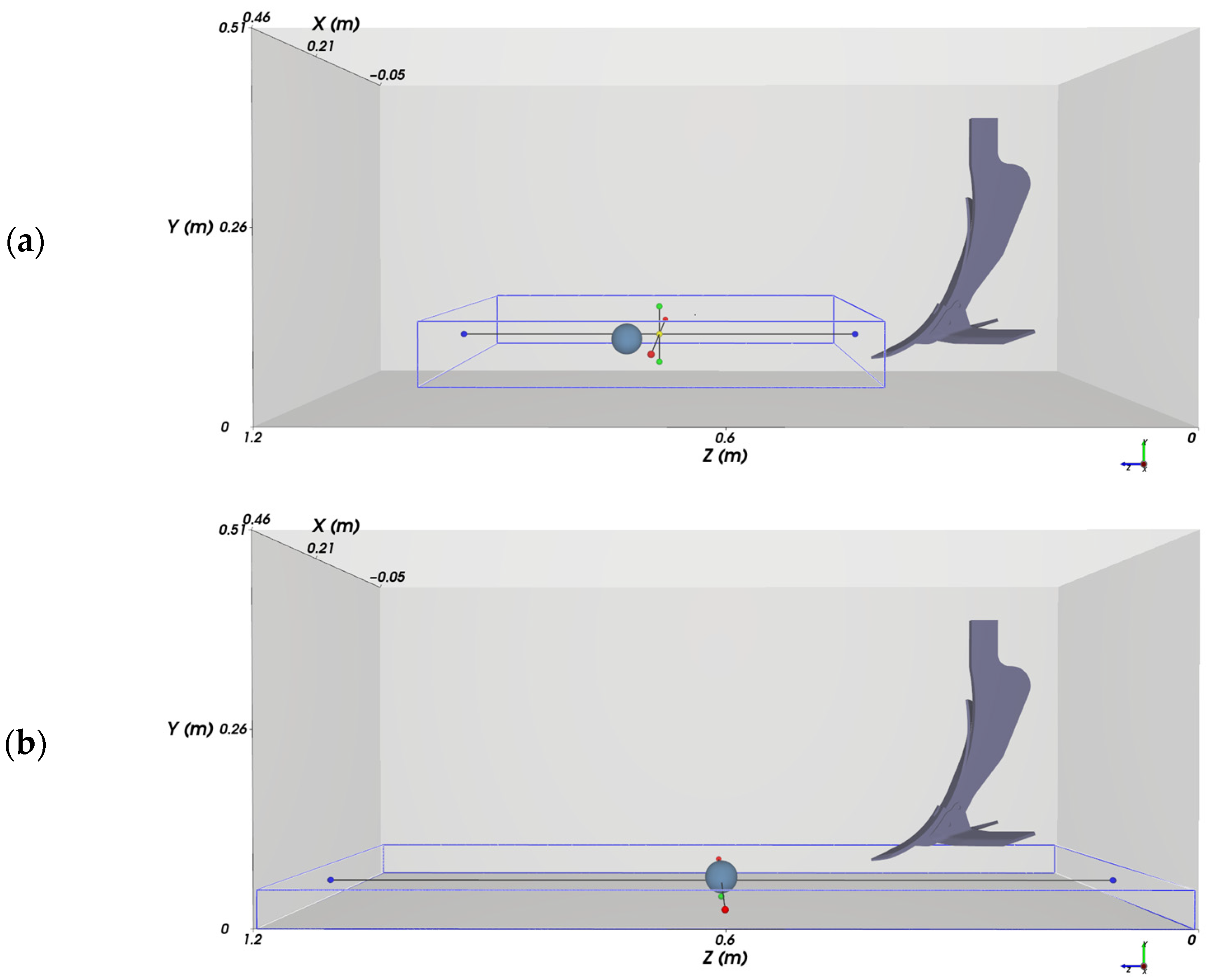
2.7.6. Particle Intlets

For the creation of the particle input, a Volumetric Inlet was chosen. Figure 9a highlights the upper particle layer, which contained 2 mm-diameter particles. This layer had the following dimensions: 500 mm × 85 mm × 600 mm. The figure shows that the tillage tool does not interact with this layer. Figure 9b shows the lower particle layer, which contained 10 mm diameter particles, with dimensions of 510 mm × 50 mm × 1200 mm. In order to achieve a lower number of generated particles, the total filling height was reduced from 240 mm to 130.3 mm. As part of the calculation, it was necessary to take into account the reduction of the total height (Y–axis) within the sand box due to the initial settling of particles. Because of that, a tillage tool offset of −4.7 mm along the Y–axis was implemented, ensuring that the tool’s penetration depth aligned with the target countersink height.

2.7.7. Motion Frame

The next step involved configuring the Motion Frame, which defined the movement of the geometry. In this case, the Motion Frame was set as a translational movement of the tillage tool along the Z–axis. The speed was set to 0.1 m·s⁻¹, corresponding to the actual speed of the tool’s movement. The movement was scheduled to occur from 0 to 12 s, ensuring the tool was in motion for the entire duration of the simulation. Once configured, the Motion Frame was assigned to the tool’s geometry.

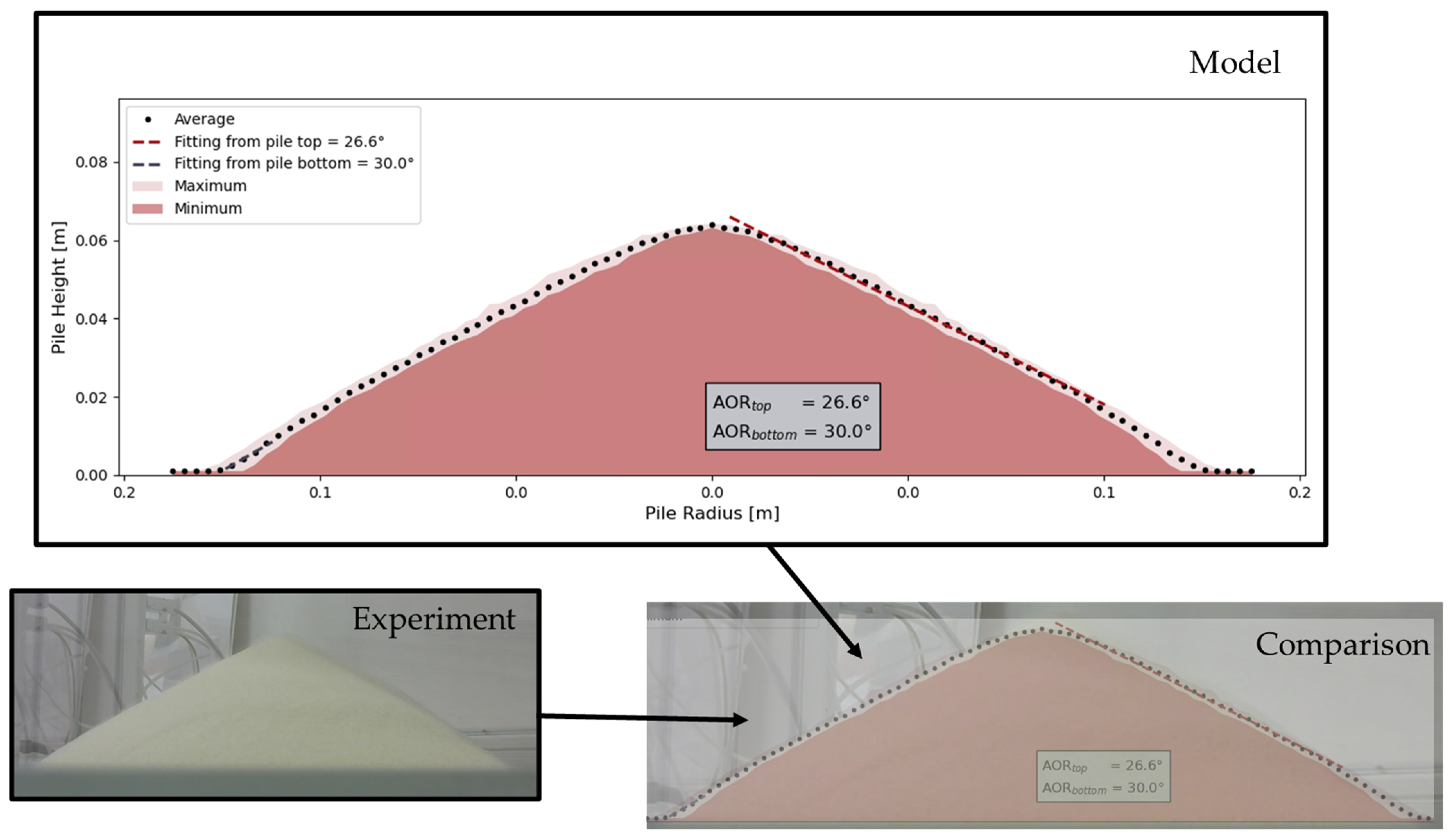
2.7.8. Model Validation Through Angle of Repose Measurements and DoE

An experiment was conducted to measure the angle of repose of sand using a laboratory experimental device specifically designed for this purpose. The methodology for the entire experiment is described in detail in study [19], which focused on rapeseed instead of sand. Following the completion of the experiment, images of the resulting sand pile were captured.

After the experiment, a DoE was proposed, consisting of 45 models. Simulation models were created to correspond to the system of the angle of repose measurement device, utilizing particulate materials. For validation purposes, the surrounding geometry model was employed, which accurately reflected the dimensions described in [19]. The simulation models followed the settings of the sand box simulation model. The parameters varied within the DoE included the Restitution Coefficient, Rolling Resistance, and Poisson’s Ratio. The ranges for these parameters within the DoE are presented in

Table 6. The ranges set within the individual parameters for DoE.

Parameter	Range
Restitution Coefficient	0.1–0.3
Rolling resistance	0.1–0.26
Poisson’s ratio	0.2–0.3

. Each model in the DoE was evaluated using a script provided by ESSS [57] to determine the static angle of repose. This script calculated average surface values for the sand pile formed and subsequently measured the angle between the sand surface and the base plate, ensuring an accurate representation of material behavior.

2.7.9. Comparison of the Traces from the Experiment and Model

To obtain particle trajectories from the Ansys Rocky software, the post-processing tool Cube was utilized, which allowed for the selection of particles located within a defined region. A custom script was developed to extract the X, Y, and Z co-ordinates of each selected particle individually from Cube.

3. Results

3.1. Obtaining X, Y, and Z Co-Ordinates in Space Using an ANN

In the preparation of the ANN, 4130 samples were allocated from a total of 44,130 data points for testing purposes.

Table 7. Comparison of neural network prediction results with actual values from the test dataset.

Parameter	Value
Average difference in mm between co-ordinates	2.3
Standard deviation of the difference in mm between co-ordinates	1.8
Maximum difference in mm between co-ordinates	10.9
Minimum difference in mm between co-ordinates	0.1
R2 Score for X co-ordinates	0.9988
R2 Score for Y co-ordinates	0.9972
R2 Score for Z co-ordinates	0.9982

presents the comparison of neural network prediction results with actual values from the test dataset.

The trained ANN model was subsequently utilized to derive trajectories from pixel values of contrasting points generated using DaVinci Resolve. The code facilitated input through two datasets: the first dataset included the pixel values from the side camera (x_s and y_s) and the second containing pixel values from the front camera (x_f and y_f). Following this process, the code enabled the export of a *.csv file containing the spatial co-ordinates X, Y, and Z.

3.2. Image Analysis for the Detection of Movements in Particulate Matter

Based on the experimental setup, eight particles were tracked and labeled from 1 to 8 (Figure 4). The tracking was conducted using DaVinci Resolve 19, where all particles except Particle 4 were successfully traced. Particle 4 became buried under a layer of sand at the onset of the traversal, preventing synchronized tracking of its movement. Consequently, its trajectory was excluded from the analysis.

Figure 10 presents a 3D chart illustrating the trajectories of the remaining seven particles. Among these, Particles 5, 6, 7, and 8 displayed movement patterns that closely aligned with expected real-world behavior. Particles 1, 2, and 3 exhibited trajectory shapes that were consistent with the anticipated path, however, the trajectories showed some distortion. This distortion was likely caused by insufficient calibration of the observed area, impacting the accuracy of their recorded paths.

Figure 11 presents the trajectories of particles 5, 6, 7, and 8. The plot reveals a clear distinction in trajectory patterns between particles 5 and 6 and particles 7 and 8. Particles 7 and 8 exhibit movement consistent with material flow, accurately following the particle transport along the system’s expected path. In contrast, particles 5 and 6 exhibited slight deviations. These deviations were likely due to slippage along the surface caused by the movement of the underlying particles. The Figure 11 shows that the trajectories of particles 7 and 8 correspond to the movement of material, alongside particles 5 and 6 exhibit displacement due to material flow. The trajectories indicate that particles 5 and 6 did not achieve the expected height along the Y–axis (m), and their displacement along the Z–axis was greater than that of the particles that were properly entrained by the material flow. Although these particles were accurately traced through optical tracking, their trajectories cannot be used to validate the movement of the model particles.

3.3. The Results of the Model Calibration

For the calibration of the model, the angle of repose method was employed. Experimental testing found that the angle of repose for silica sand ranged from 28.8° to 32.9°, giving an average value of 31°. This angle of repose was used to adjust the model parameters accordingly.

A DoE approach was conducted, which included variable parameters such as the Restitution Coefficient, Rolling Resistance, and Poisson’s Ratio. The optimal combination of these parameters was evaluated both on the basis of the measured angle of repose and on the basis of the resulting shape of the sand pile created during the simulations. Finally, model number 40 was selected as the best configuration with specific parameter settings detailed in

Table 8. Parameter settings from DoE for model number 40.

Parameter	Range
Restitution Coefficient	0.3
Rolling resistance	0.26
Poisson’s ratio	0.25

.

Figure 12 presents a comparison between the experimental sand pile and the results from the Ansys Rocky script. The image from the experiment was created by combining a total of 12 images taken from different rotational angles, to provide an analogous comparison to the approach used in the Ansys Rocky script. From the figure, the results obtained from the script are also evident, showing the average and maximum values on the Y–axis in relation to the X– and Z–axes on the surface of the pile. Additionally, the figure provides the measured angle of repose at both the base and the top of the pile, along with the maximum and minimum particle occurrence values along the Y–axis based on the X and Z positions on the pile’s surface. Lastly, the figure shows an overlay of both images, which confirms not only the agreement in the angle of repose (30°) but also the matching shape of the pile.

3.4. The Simulation Model Calculation

Based on the results from the DoE, a complete simulation model was configured. The developed and computed simulation model of the tillaging as the result of the digital twin of the system is shown in Figure 13b in comparison to the experiment (a). The total memory usage for the simulation was approximately 100 GB, with a computation time of 10 h, 48 min, and 50 s. The simulation involved a total of 3,634,586 particles. Each particle was assigned a unique ID number (ID 1 to ID 3,634,586). The time step for the calculation was set to 1.7 × 10⁻⁵ s. The total simulation time was set to 6 s.

3.5. Comparison of the Traces from the Experiment and the Model

Within this study, trajectories derived from Ansys Rocky (Particle ID) were compared with those obtained via image analysis. For each tracked point, corresponding particles in the DEM model were identified based on initial co-ordinates. Particles were located at the same positions as the tracked particles from the experiment. Therefore, these particles were used for comparison. To obtain particle trajectories from the Ansys Rocky software, the Cube tool was employed, allowing for the generation of trajectories from the specified region. These trajectories were then graphically represented on Y (m)—the vertical axis, Z (m)—the tillage tool movement axis, and on X (m)—the horizontal axis to Z (m)—the tillage tool movement axis. The model trajectories were further overlaid with trajectories obtained from image analysis for comparison.

Given the slight nuances in the positioning of particles in the sand box along the X–axis, particles 7 and 8 were compared with particles corresponding to their actual locations. ID 462069 was considered for both particles. Particle 7 was compared with particles ID 448375, ID 462061, and ID 462069. Particle 8 was compared with particles ID 448371, ID 462069, and ID 475956.

Figure 14 presents a graph comparing the trajectory of particle 7, as obtained through image analysis, with trajectories derived from Ansys Rocky in the Y– and Z–axes. To ensure clearer comparison, the initial values for particles from the DEM model and those from the experiment were set to zero. The figure shows, that all particles, both from the model and the experiment, exhibit a similar upward trend along the Y–axis as their position increases along the Z–axis. The trajectory lengths were represented in the graph with a length of 0.2 m. A slight nuance was observed at the end of the course, where the standard deviation on the Z–axis at 0.18 m reached 0.015 m. All routes corresponded in shape up to 0.179 m on the Z–axis, where particles ID 448375 and ID 462069 began to drop sharply during the course. This was due to the fact that they were already in the sliding phase. Particle number ID 462061 corresponded most in shape to particle 7.

A graph for the same particle, shown on the X– and Z–axes in Figure 15, illustrates that the particle’s trajectory aligns within the dispersion of neighboring particles. Since these particles were close to the tillage tool’s central axis, their dispersion spread symmetrically across both sides of the processed material. This is most evident for particle ID 462061, whose value on the X–axis extended into negative values. Despite this, it was demonstrated that the particles closely matched the experimental trajectory, and at 0.18 m on the Z–axis (in the sliding phase), the standard deviation was 0.0261 m.

The same comparisons as for the particle 7 are depicted for particle 8 on the Y– and Z–axes in Figure 16 and on the X– and Z–axes in Figure 17, providing further verification of the model’s trajectory consistency. The trajectory lengths were again represented in the graph up to a length of 0.2 m. In this case, the trajectories aligned most closely up to 0.14 m on the Z–axis, where the particles in the model transitioned into the sliding phase. At this distance on the Z–axis, the standard deviation on the Y–axis was 0.002 m for all particles, with particle ID 475956 most closely matching the shape of particle 8. Among the particles, particle ID 448371 was the first to transition into the sliding phase, exhibiting a negative trend on the X–axis (Figure 17). The standard deviation on the X–axis was 0.027 m, with particle ID 448371 having the most significant numerical influence.

4. Discussion and Conclusions

In our study, an effective method was developed for verifying particulate system models on particle movement, which enables a better understanding and more accurate prediction of their behavior. Nowadays, as digitalization and advanced technologies become more prevalent, real-world processes are often simulated using digital twins. This approach eliminates the need for complex experiments, which are typically influenced by factors such as weather, agrotechnical timing, measurement accuracy, and economic costs. DEM models offer the advantage of easily tracking particle trajectories, which is generally very difficult under real conditions. To use these models for this purpose, they must first be verified. Our study focuses on advancing the application of neural networks by proposing their use as a novel approach for verifying particle movements in DEM models. While numerous studies have explored neural networks as tools for predicting the outcomes of DEM simulations [51,52,53].

To determine spatial co-ordinates in our study, we used the Caliscope software [48], which provided us with 44,130 points in space based on pixel values. Combining results from Caliscope with an ANN for regression proved to be a simple and highly effective solution.

The results of the ANN from our study indicate a high degree of accuracy, with an average co-ordinate difference of 2.3 mm and coefficient of determination (R²) of 0.9988 for the X–axis, 0.9972 for the Y–axis, and 0.9982 for the Z–axis. The standard deviation of the difference between the predicted and actual co-ordinates was 1.8 mm. Such precision demonstrates the potential of neural networks in image processing tasks, especially in dynamic environments involving particulate matter.

The trajectories of particles 1, 2, and 3, which, despite showing expected trajectory shapes, exhibited some distortions. This distortion likely resulted from insufficient calibration of the observed area, emphasizing how sensitive particle tracking can be to the calibration process. This distortion was probably mainly caused by the lateral particles being placed too close to the lateral camera. Future studies will focus on utilizing a larger sand box to mitigate these issues. A comparison of the particle trajectories obtained from Ansys Rocky model and the experimental data and image analysis in our research showed a strong similarity for particles 7 and 8. Particles 7 and 8 exhibit movement consistent with material flow, accurately following the particle transport along the system’s expected path. In contrast, particles 5 and 6 exhibited slight deviations. These deviations were likely due to slippage along the surface caused by the movement of the underlying particles. Although these particles were accurately traced through optical tracking, their trajectories cannot be used to validate the movement of the model particles.

The methodology was applied to dry sand, where particle movement was observed as it passed through a tillage tool. Dry sand was chosen for its simplicity compere to more complex particulate systems. A significant contribution of this study is that the proposed methodology enables the repeatable application of the entire calibration system for the verification of various particulate materials with different properties and compositions, potentially allowing for the verification of highly complex, variable, and diverse structures, as is the case with soils. A requirement is to maintain geometries, positions, and camera settings while changing the particulate substance within the experiment, as well as the input parameters based on the verified particulate system. This research effectively illustrates the successful integration of ANN with particle tracking methodologies, achieving a high level of accuracy in spatial co-ordinate estimation. The results highlight the importance of rigorous calibration and validation approaches, which can contribute to the development of more sophisticated and accurate prediction frameworks. The study further confirms the reliability of the application of image analysis and neural networks for tracking the movement of particles in particulate materials for the validation of DEM models.

The key findings of this study are as follows:

• A methodology for obtaining spatial co-ordinates employing a combination of stereoscopic triangulation using Caliscope software and ANN for regression was proposed. This combination has proven to be a simple and highly effective approach;
• The neural network analysis demonstrated high accuracy, achieving R² values of 0.9988, 0.9972, and 0.9982 for the X–, Y–, and Z–axes, respectively. The standard deviation between predicted and actual co-ordinates was found to be 1.8 mm;
• A comparison of the particle trajectories from the model and experiment revealed a strong agreement;
• The proposed method is applicable for the verification of various materials while maintaining the geometries, positioning, and settings of the cameras.