Article

A Comparison of Monte Carlo-Based and PINN Parameter Estimation Methods for Malware Identification in IoT Networks

by
Marcos Severt
1,
Roberto Casado-Vara
2,* and
Angel Martín del Rey
3
1
Campus of Sciences, Universidad de Salamanca, Pl. Caídos, s/n, 37008 Salamanca, Spain
2
Grupo de Inteligencia Computacional Aplicada (GICAP), Departamento de Matemáticas y Computación, Escuela Politécnica Superior, Universidad de Burgos, Av. Cantabria s/n, 09006 Burgos, Spain
3
Department of Applied Mathematics, Universidad de Salamanca, 37008 Salamanca, Spain
*
Author to whom correspondence should be addressed.
Technologies 2023, 11(5), 133; https://doi.org/10.3390/technologies11050133
Submission received: 10 August 2023 / Revised: 13 September 2023 / Accepted: 25 September 2023 / Published: 30 September 2023
(This article belongs to the Topic Cyber-Physical Security for IoT Systems)

Abstract

:
Malware propagation is a growing concern due to its potential impact on the security and integrity of connected devices in Internet of Things (IoT) network environments. This study investigates parameter estimation for Susceptible-Infectious-Recovered (SIR) and Susceptible–Infectious–Recovered–Susceptible (SIRS) models modeling malware propagation in an IoT network. Synthetic data of malware propagation in the IoT network is generated and a comprehensive comparison is made between two approaches: algorithms based on Monte Carlo methods and Physics-Informed Neural Networks (PINNs). The results show that, based on the infection curve measured in the IoT network, both methods are able to provide accurate estimates of the parameters of the malware propagation model. Furthermore, the results show that the choice of the appropriate method depends on the dynamics of the spreading malware and computational constraints. This work highlights the importance of considering both classical and AI-based approaches and provides a basis for future research on parameter estimation in epidemiological models applied to malware propagation in IoT networks.

1. Introduction

In an era of ever-expanding information technology and connectivity, cybersecurity has become a key concern [1]. An environment conducive to the proliferation of cyber threats has been created by the increasing interconnectedness of devices and systems through Internet of Things (IoT) networks [2,3]. This interconnectivity, through the integration of smart devices into large-scale networks, has enabled the transformation of virtually every aspect of society, from industry and healthcare to people’s daily lives. With this technological revolution have come cybersecurity challenges [4]. New attacks and vulnerabilities have emerged due to the breadth and diversity of IoT devices and their ability to exchange data and communicate with each other. One of the most pervasive and difficult to prevent threats is malware [5]. Malware comes in many forms, ranging from malicious software that steals sensitive information to code designed to disable systems and launch distributed denial of service (DDoS) attacks [6]. To ensure the security, privacy, and reliability of IoT networks, the need to effectively detect and mitigate these threats has become a critical imperative. Cyberattacks can have devastating consequences, from disrupting essential services to exposing sensitive data and undermining trust in digital systems [7]. As the IoT ecosystem continues to grow, the need for effective defense against malware and other cyberthreats is becoming more urgent than ever. Applying epidemiological models tailored to malware propagation in IoT networks offers a promising approach to understanding and mitigating these threats [8]. Through the use of concepts and methods from epidemiology, it is possible to take into account the dynamics of malware propagation and develop proactive defense strategies. A crucial step in the application of these epidemiological models to real data is the estimation of propagation model parameters such as transmission rate and recovery rate in the SIR model. There are a number of methods in the literature that have been widely used by researchers to estimate these parameters, including curve fitting [9,10], least squares [11,12], maximum likelihood [13,14], Monte Carlo Markov chain [15,16], and PINNs [17,18], to name a few. The method chosen for estimation depends on the available data, complexity of the model, and nature of the epidemic. In practice, several approaches are often combined to obtain more accurate and robust estimates of the propagation model parameters. Certain methods, such as PINNs and Monte Carlo-based methods, have very useful advantages when only the number of infections over time is available. These include adaptability to irregular data, incorporation of physical equations, scalability, uncertainty estimation, or exploration of parameter space, among others. However, in the same cases, where all that is available is the number of infections over time, maximum likelihood and least squares have relevant disadvantages as well, namely, high sensitivity to outliers, no information about uncertainty, non-optimality for non-normal distributions, the need to know the distribution, lack of an available likelihood function, etc. For this reason, we decided to compare PINNs and Monte Carlo methods in this study, while excluding maximum likelihood and least squares methods from the comparison. Comparing methods based on Monte Carlo techniques and Physics-Informed Neural Networks (PINNs) for parameter estimation in SIR/SIRS models provides a unique opportunity to determine which approach can provide robust and efficient defense in detecting and mitigating malware in IoT networks.
Identifying malware spreading through IoT networks is crucial for developing effective cyberattack mitigation strategies. Existing methodologies involve estimating parameters in epidemiological models; however, estimating these parameters is challenging due to the inherent difficulties in understanding and modeling malware characteristics [19]. Accurately identifying malware parameters, such as propagation and recovery rates, is crucial for anticipating behavior and implementing countermeasures. The limited availability of actual attack data complicates cybersecurity efforts. Due to the sensitive nature of the information and the lack of access to comprehensive records of security incidents, obtaining representative datasets becomes a daunting task. This hampers the capabilities of traditional estimation methods, which often rely on large and diverse datasets to produce reliable results. The lack of relevant data can lead to inaccurate parameter estimates, ultimately limiting the effectiveness of model-based defense strategies. Overall, overcoming the challenges of parameter estimation in cybersecurity requires approaches that can cope with uncertainty and incomplete data. The use of adaptive and flexible methods is essential for the development of robust and reliable cyberdefense systems in a constantly evolving environment [20]. Epidemiological models, such as the SIR and SIRS approaches, are used to understand and predict the spread of disease in populations. The SIR model divides individuals into three compartments, namely, susceptible, infected, and recovered, assuming that when recovered they cannot be reinfected. The SIRS model adds an additional compartment for individuals who become susceptible again after recovery. These models can be adapted to analyze the spread of malware in IoT networks, where devices are considered susceptible, infected, and recovered. The spread of malware depends on factors such as device interaction and defense effectiveness. Adapting SIR and SIRS models to cybersecurity provides a deeper understanding of malware propagation and a framework for estimating critical parameters such as infection rate and recovery rate. This adaptation offers a new perspective for analyzing and designing defense strategies against cyberthreats in an increasingly connected environment.
The security of Internet of Things networks is a critical challenge in the digital domain. From data loss to disruption of critical services, the spread of malware across these networks can be devastating. In order to combat this problem, it is essential to understand how malware spreads. The estimation of the parameters in malware propagation models provides us with an invaluable tool for the anticipation, prevention, and mitigation of attacks. It is possible to identify patterns and trends, evaluate the effectiveness of security measures, and develop more efficient strategies to protect IoT networks by knowing the number of people infected over time. This work is not only fundamental to cybersecurity; it helps advance computing and protect privacy in an increasingly connected world. The main objective of this study is to perform an exhaustive comparison between two parameter estimation methods based on Monte Carlo techniques and a PINN in the context of SIR/SIRS models adapted to describe malware propagation in IoT networks. In the field of cybersecurity and parameter estimation, the highlights of this research are the following:
  • Our study provides a detailed and rigorous comparative evaluation of two well known approaches to parameter estimation.
  • We identify the benefits of both approaches as well as the time required to perform parameter estimation. This information can help cybersecurity professionals to make informed decisions and develop more efficient strategies to protect IoT networks.
  • We hope to inspire other researchers to further explore the intersection of epidemiology, cybersecurity, and data science by highlighting the benefits and limitations of each approach.
Overall, our contributions aim to enrich the field of cybersecurity by providing a robust comparative assessment and highlighting the utility of modeling techniques in mitigating digital threats in IoT networks. This paper is organized as follows. Next, we present the materials and methods in Section 2. Section 3 presents the setup of our simulations and the results, along with a performance comparison of selected methods. Finally, Section 4 concludes the conducted research and proposes future lines of work.

2. Materials and Methods

2.1. Synthetic Data

The relevance of policy advice depends on the ability of a model to capture the essential aspects of the system that are relevant to the problem at hand [21,22]. However, modelers face a dilemma in determining the importance of each aspect. In [23], the metaphor of large and small worlds was used to illustrate this process. The large world represents a complex entity with partial, confusing, and ambiguous information. Models are designed to understand, influence, manage, and control this intricate complexity [24]. On the other hand, the small world refers to the self-contained logical reality of the model, where comprehensive corrective actions can be taken and their consequences tested under both favorable and extreme conditions [25]. However, these logical consistency tests are limited to the small world and cannot be directly applied to the large world. Validation procedures are used to increase confidence in the applicability of the model to the large world. However, navigating between these two worlds and recognizing their differences remains a fundamental challenge in modeling. Finding the right balance and ensuring the relevance of the model to the complexities of the real world is essential for effective policy advice [26,27].
In epidemiological model identification, the large world is the data-generating process, encompassing ecological interactions that contribute to infectious disease spread. However, partial observations of this activity are limited. Incidence reports from surveillance entities can provide time series data for model selection, which can be used to obtain parameter estimates [28,29]. However, generating accurate incidence rates from a model is not enough for validity, as it does not guarantee that all relevant factors have been considered or that parameter estimates are close to actual quantities. To address this issue, synthetic data can be used to represent the large world and ensure that both worlds are perfectly aligned. The model used to estimate parameters is structurally identical to the data generation process, preventing inconsistencies in the calibration process. The data generation process is grounded in previous research in the field, and the workflow from producing synthetic age-specific incidences to parameter estimation is detailed in [30].

2.2. Data Generation and Mathematical Models

Mathematical models can simulate malware propagation based on models developed to study infectious diseases. These models are compartmental, dividing the population into different types of behavior based on disease characteristics. In the case of malware propagation, these categories include susceptible, exposed, infectious, quarantined, and recovered. These models can help to understand the dynamics of infection and its impact on networks [31,32]. Such models include Susceptible–Infectious–Susceptible (SIS), Susceptible–Infectious–Recovered (SIR), Susceptible–Infectious–Recovered–Susceptible (SIRS), Susceptible–Exposed–Infectious–Recovered (SEIR), and SI and SIRS variants, to name only a few [33,34]. The SIR and SIRS models are described in detail below.
SIR Model
The SIR system is a mathematical model used in epidemiology to describe the spread of infectious diseases in a population. It has three main compartments: Susceptible (S), Infected (I), and Recovered (R). The key hyperparameters are the transmission rate ( β ), which represents the rate at which susceptible individuals become infected upon contact with infected individuals, and the recovery rate ( γ ), which represents the rate at which infected individuals recover and move to the recovered compartment. These hyperparameters are fundamental to understanding how an epidemic evolves, as they determine the dynamics of the disease. By varying β and γ , different epidemiological scenarios can be analyzed and disease control strategies evaluated. Here, S 0 , I 0 are the initial values for S and I in time 0, i.e., R ( 0 ) , I ( 0 ) .
d S d t = β S I
d I d t = β S I γ I
d R d t = γ I
S ( 0 ) = S 0 , I ( 0 ) = I 0 , R ( 0 ) = 1 S 0 I 0
SIRS Model
The SIRS system is a mathematical model used in epidemiology to describe the dynamics of infectious disease in a population. It has three main sections: “Susceptible” (S), individuals who are susceptible to infection; “Infectious” (I), infected individuals who are capable of transmitting disease; and “Recovered” (R), individuals who have recovered from infection and may become susceptible again over time. The SIRS system is characterized by several key hyperparameters: the transmission rate β , which represents the rate of infection; the recovery rate γ , which represents the speed of recovery; and the rate of loss of immunity μ , which models the gradual loss of immunity over time. These hyperparameters determine the dynamics of the system, and are critical for predicting disease spread and evaluating control strategies; S 0 , I 0 are the initial values for S and I in time 0, i.e., R ( 0 ) , I ( 0 ) .
d S d t = β S I + δ R
d I d t = β S I γ I
d R d t = γ I δ R
S ( 0 ) = S 0 , I ( 0 ) = I 0 , R ( 0 ) = 1 S 0 I 0

2.3. Propagation Model Identification Methodology

While mathematical epidemiology can model the propagation of malware in a network by requiring knowledge of the propagation dynamics, in reality, when malware is detected the most readily available information is the number of infections in the network. This means that in order to understand its propagation dynamics and mitigate its impact, the first task when malware is discovered in a network is to identify it. Several techniques exist in the literature for this purpose, mainly based on statistical techniques and optimization [35,36,37,38,39]. A new strategy for estimating the parameters of dynamical systems using deep learning has emerged in recent years. This technique consists of using neural networks, with the loss function modified to take into account the equations that define the dynamical systems. These neural networks are called PINNs, and are first described in [40]. PINNs have been widely used to estimate the parameters of mathematical epidemiological models used for modeling COVID-19 and performing parameter estimation [18,41], as well in other fields [42,43,44]. After reviewing the state of the art, we propose a comparison between Monte Carlo-based methods and PINNs to estimate the parameters of mathematical models in order to accurately identify the dynamics of malware propagation in networks. This approach was chosen because, among statistical parameter estimation techniques, Monte Carlo-based inference has proven to be the most efficient; on the other hand, among the parameter estimation techniques based on artificial intelligence, PINNs have proven to be the most efficient. When the parameters of all known models have been estimated, the shape of the infectee curve produced by the ideal model and the infectee curve measured in the network with an MSE are evaluated. Note that the parameters must be between 0 and 1, otherwise, the model must be rejected. Assuming that δ > 0 is the tolerance, it can be assumed that if the MSE of both curves is less than δ , we have successfully modeled the spread of malware through the network. If none of the epidemiological models match the one that is spreading in the network, it can be assumed that it is an unknown model, at which point the task becomes modeling it mathematically and studying its stability and equilibrium points.

2.3.1. Monte Carlo Method

We designed a Monte Carlo algorithm to estimate the parameters of the models described in Section 2.2. In order to apply the theory of statistical inference, we assume that the parameters are random variables when designing algorithms based on Monte Carlo techniques [45]. The goal is to estimate the posterior distribution of the parameters, referred to as π ( θ | y ) , or the target distribution in the context of Bayesian analysis. The aim is to locate the target distribution within the parameter space, i.e., to locate the regions of the probability mass that describe the observations y, which can be described as calculating the expectation of g:
E π ( g ) = g ( θ ) π ( θ | y ) d θ .
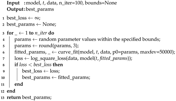
In rare cases, it is possible to solve the expected value of a function analytically. However, when this is not possible, simulation methods can be used. When using simulation, there is a general solution. This involves using Markov Chain Monte Carlo (MCMC) techniques to estimate the quantities of interest. Using Markov chain simulations, the desired values can be effectively calculated by simulating either from the true distribution or some suitable surrogate distributions [46,47]. In order to improve the estimation accuracy of the developed algorithms, two loss functions are used: the mean square error (see Algorithm 1), and another based on the log square error (see Algorithm 2). Both algorithms have the same design, and rely on knowledge of malware propagation models to estimate the unknown parameters using statistical inference with MCMC. In this way, a sample of up to 50,000 cases is generated, and the algorithm’s solution to the infection curve is compared with measurements taken from the network.
Algorithm 1: Monte Carlo parameter estimation with MSE loss function
Technologies 11 00133 i001
Algorithm 2: Monte Carlo parameter estimation with log square loss function
Technologies 11 00133 i002

2.3.2. Physics-Informed Neural Networks

This section is based on the work conducted by Raissi et al. in Section 2 and Section 4 of [40]. Their work uses deep neural networks as universal function approximators [48] to tackle nonlinear problems without prior assumptions or linearisation. Automatic differentiation techniques are used to differentiate neural networks with input coordinates and model parameters [49], resulting in physics-informed neural networks. This approach addresses various computational problems and introduces transformative technology for data-efficient and physics-informed learning machines, numerical solvers, and data-driven approaches for model inversion and system identification. In this work, we consider parameterized and nonlinear partial differential equations of the general form
u t + N [ u ; λ ] = 0 , x Ω , t [ 0 , T ] ,
where u ( t , x ) denotes the latent (hidden) solution, N [ u ; λ ] is a nonlinear operator parameterized by λ , and Ω is a subset of R D . To illustrate how PINNs work, we examine the case of the SIR model, i.e., we detail the data-driven parameter discovery for the SIR model.
Let t R + be the input of the PINN, and let f ( t ; θ ) R + m + 1 be the output of the PINN, where m is the number of hidden layers. Based on the Kermack and McKendrick model [50], the PINN model has the basic three-compartment SIR model with their parameters. Then, the PINN output is
f ( t ; θ ) = f 1 ( t ; θ ) f 2 ( t ; θ )
where f 1 ( t ; θ ) , f 2 ( t ; θ ) approximates S ( t ) , I ( t ) , respectively. Note that R ( t ) is completely determined by the others, as R = N S I . Then, we can reduce the computational complexity by reducing the system [ S ( t ) , I ( t ) ] T shown in [18]. Assuming that no data are available for compartments S and R and that { u k } k = 0 K is a discrete-time series of observations in compartment I at time t k , the MSE data loss is defined as
M S E d a t a = 1 K + 1 k = 0 K ( u k f 2 ( t k ; θ ) ) 2
where MSE is the loss function.
Then, the inverse problem can be described as follows. For an incomplete dataset, the PINN aims to learn a mapping from time t to each of the state variables in the existing model. Thus, using the incomplete dataset, we can extrapolate the unknown time series of the S and R compartments and learn the transmission dynamics represented by the values of the SIR parameters β and γ . The PINN must access information from the pre-existing model during training (i.e., the SIR model). Then, the subsystem can be written as
G y , d y d t ; λ = d y d t + N [ y ] = 0 ,
where N [ · ] is generally a differential operator (though in the case of ordinary differential equations it is possible for N [ · ] to represent a nonlinear function of the variable y) and
y ( t ) : = S ( t ) I ( t ) , d y d t = d S ( t ) d t d I ( t ) d t , N [ y ] = β N S I β N S I + γ I .
If N [ y ; λ ] depends on λ = ( β , γ ) T R 2 with λ that are not known a priori, then
G ( y , y t ; λ ) = y t + N [ y ; λ ] , t [ 0 , T ] .
Therefore, in order to train the PINN effectively we need to minimize targets of the following form:
m i n θ , λ ( M S E d a t a ( θ ) + M S E G ( θ , λ ) ) ,
enabling the PINN to learn the model parameters from the data [18,40].
Note that if the system has initial conditions, then the function to be minimized is
m i n θ , λ ( M S E d a t a ( θ ) + M S E G ( θ , λ ) ) + M S E I C ( θ ) .
Here, we have constrained the parameters to be time-independent. If they were time-dependent, it would be necessary to create a sliding window with an amplitude of α Δ t with α R to be passed as input to the PINN small frames as follows: ( t , t + α Δ t ) . For the remaining models, it is sufficient to substitute the SIR equations for the model equations to be studied.

3. Results and Discussion

This section presents and analyses the results of comparing two different approaches for estimating malware propagation model parameters in a network, namely, Monte Carlo (with both loss functions) and PINNs. The performance of both methods is evaluated in terms of their ability to estimate the parameters of the malware propagation model on the basis of the infection curves generated in the network.

3.1. Experimental Setup

In order to compare the proposed methods, synthetic data were generated for the selected malware propagation models SIR and SIRS; we chose these models because they have the same compartments. The odeint Python function was used to generate the synthetic data. This function applies the Runge–Kutta numerical method ( 4 , 5 ) to the systems of equations of the propagation models, and as a result provides the sequences of solutions. In the case of the SIR model, it provides the solutions of susceptible (S), infected (I), and recovered (R); for this comparison, however, we are only interested in the infected, as in the real world there is usually only access to these measurements. Finally, we evaluated the malware propagation models at time interval t [ 0 , 2000 ] . To compare the two approaches, the following data preprocessing steps were performed: (1) synthetic infected curves were generated using the malware propagation model in a simulated network, varying the parameters of interest; (2) artificial noise was added to the infected curves to simulate real-world conditions and increase the complexity of the estimation task using NumPy’s ’random.normal’ function, and the Monte Carlo method (with both loss functions) was programmed in Python by creating two custom functions, as shown in Algorithms 1 and 2; finally, the PINN test was conducted in Python with the deepxde library to code the PINNs [51] on a desktop (CPU: Intel (R) Core (TM) i7-8700 CPU @ 3.20 GHz; Memory: 16 GB; OS: Microsoft Windows 10 with 64 bits). PINNs have an input layer of a single neuron, three hidden layers of 40 neurons each, and an output layer of three neurons. The activation function is ‘tanh’ and the initialization of the neural network weights is ‘Glorot uniform’. The optimizer was ‘Adam’, with a learning rate of 0.001 and beta and gamma as the ‘external trainable variables’. The PINN had 10,000 iterations on the data provided to it in each algorithm parameter estimation training loop. Finally, before starting the experiments for both scenarios, two PINNs were trained, one with the SIR model and the other with the SIRS model. Therefore, both PINNs were used in both scenarios and their performance was investigated.

3.2. SIR Parameter Estimation

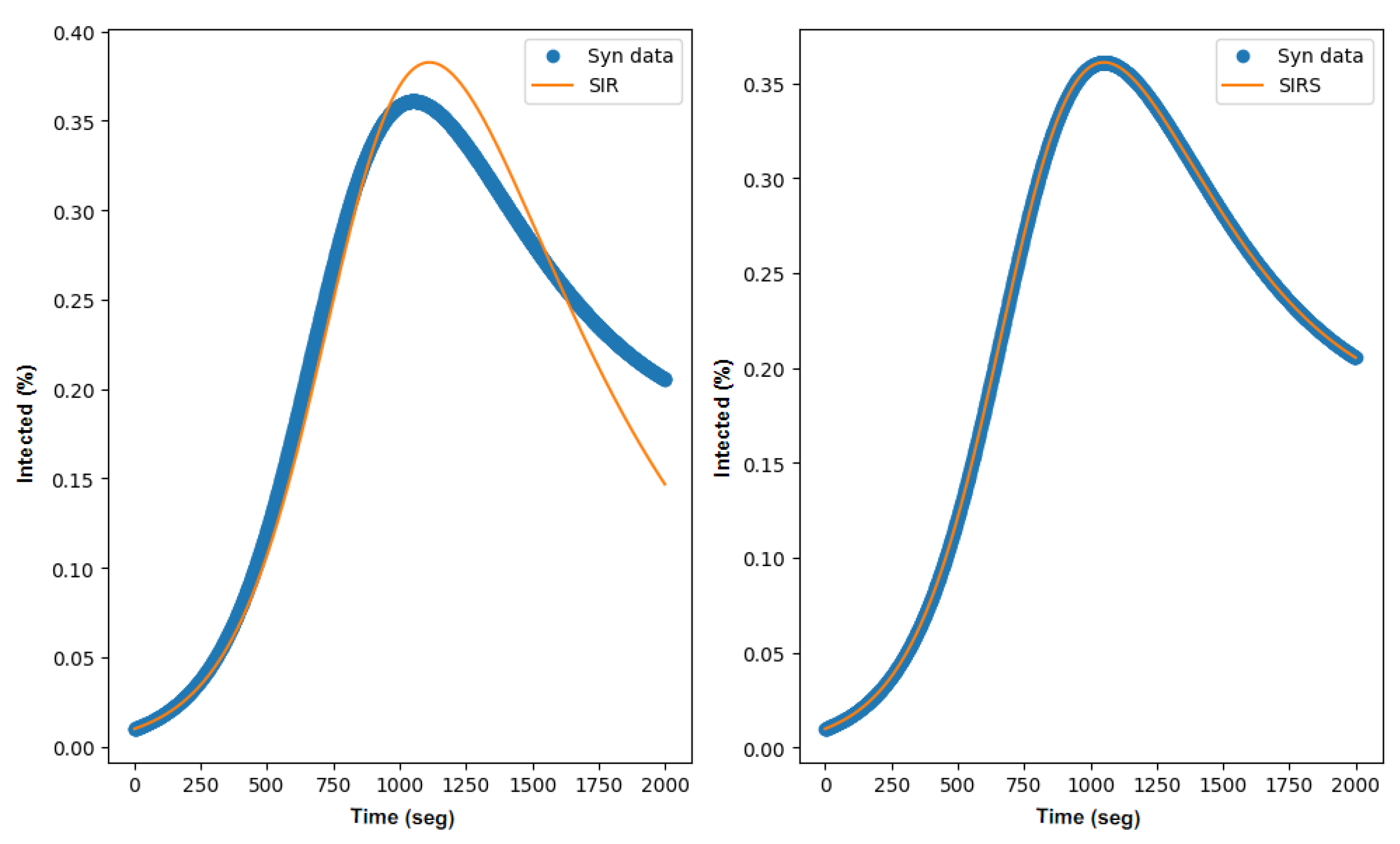
Consider malware propagating through a network according to a SIR model. In this experiment, the initial conditions were S ( 0 ) = 0.99 , I ( 0 ) = 0.01 , and the parameters were β = 0.8 and γ = 0.25 with time t [ 0 , 2000 ] . Figure 1 shows the results of the method Monte Carlo MSE (MC MSE). It can be seen that the MC MSE method estimates the parameters after 52 s and generalizes the infected curve with the SIR (left) and SIRS (right) models. The MC MSE method correctly identifies that the malware in this experiment follows the SIR model, as can be seen in this figure.
On the other hand, the model followed by the malware in this experiment follows the SIR model, according to the Monte Carlo model with a log-square loss function, which estimates the parameters after 56 s (see Figure 2).
The results obtained in this experiment by the PINNs trained with the SIR model (Figure 3 top left) and SIRS model (Figure 3 top right) show that they are able to estimate the parameters in such a way that the infected curve produced by the PINN is equal to the one measured in the network. However, in the parameter estimation, the PINN trained with the SIRS model correctly estimates the parameters (Figure 3 bottom left); the PINN trained with the SIR model (Figure 3 bottom right) correctly estimates β and γ , while for δ it provides a different value in each simulation that is very close to 0 and sometimes even negative. To illustrate this example, we have taken the average of the δ obtained in ten simulations. The PINN trained with the SIR model took 154 s to estimate the parameters, while the PINN trained with the SIRS model took 163 s.
Finally, a comparison of the estimates from the three methods compared in this study can be seen in Table 1. Both Monte Carlo-based methods correctly estimate the parameters of the SIR model while finding parameters for the SIRS model that are outside the bounds of these parameters, i.e., 0 β , γ , δ 1 . On the other hand, PINN-SIR correctly identifies the parameters, whereas PINN-SIRS is not able to estimate them, as was expected based on to its training.

3.3. SIRS Parameter Estimation

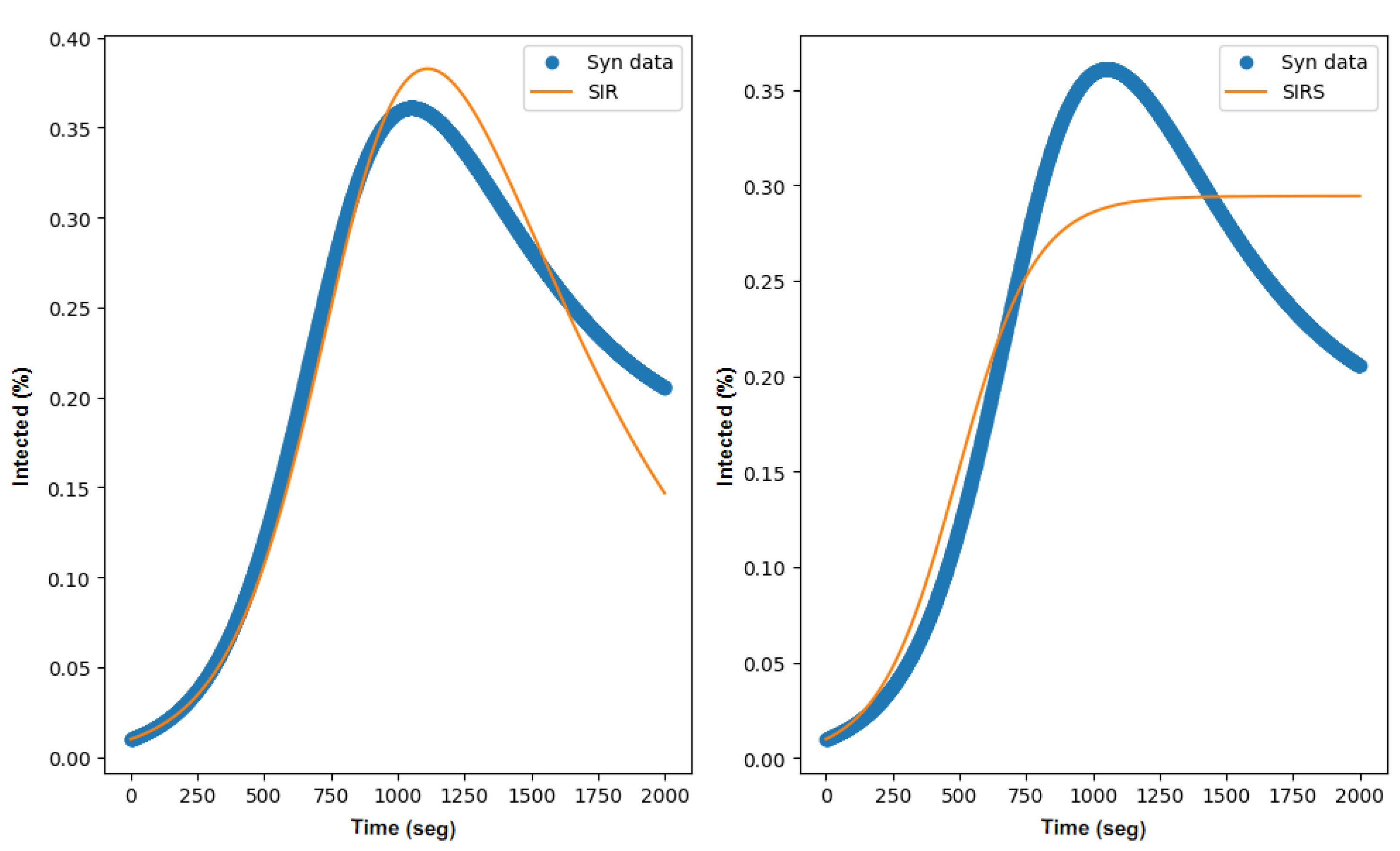
Consider malware propagating through a network according to the SIRS model. In this experiment, the initial conditions were S ( 0 ) = 0.99 , I ( 0 ) = 0.01 and the parameters were β = 0.8 , γ = 0.25 and δ = 0.1 with time t [ 0 , 2000 ] . Figure 4 shows the results of the MC MSE. It can be seen that the MC MSE method estimates the parameters after 53 s and generalizes the infected curve with the SIR (left) and SIRS (right) models. The MC MSE method cannot identify that the malware in this experiment follows a SIR model, although it can identify the parameters of a SIRS model.
In the case of the Monte Carlo log-square method, Figure 5 shows that it cannot correctly estimate the parameters of either the SIR or SIRS model. This estimation took 71 s.
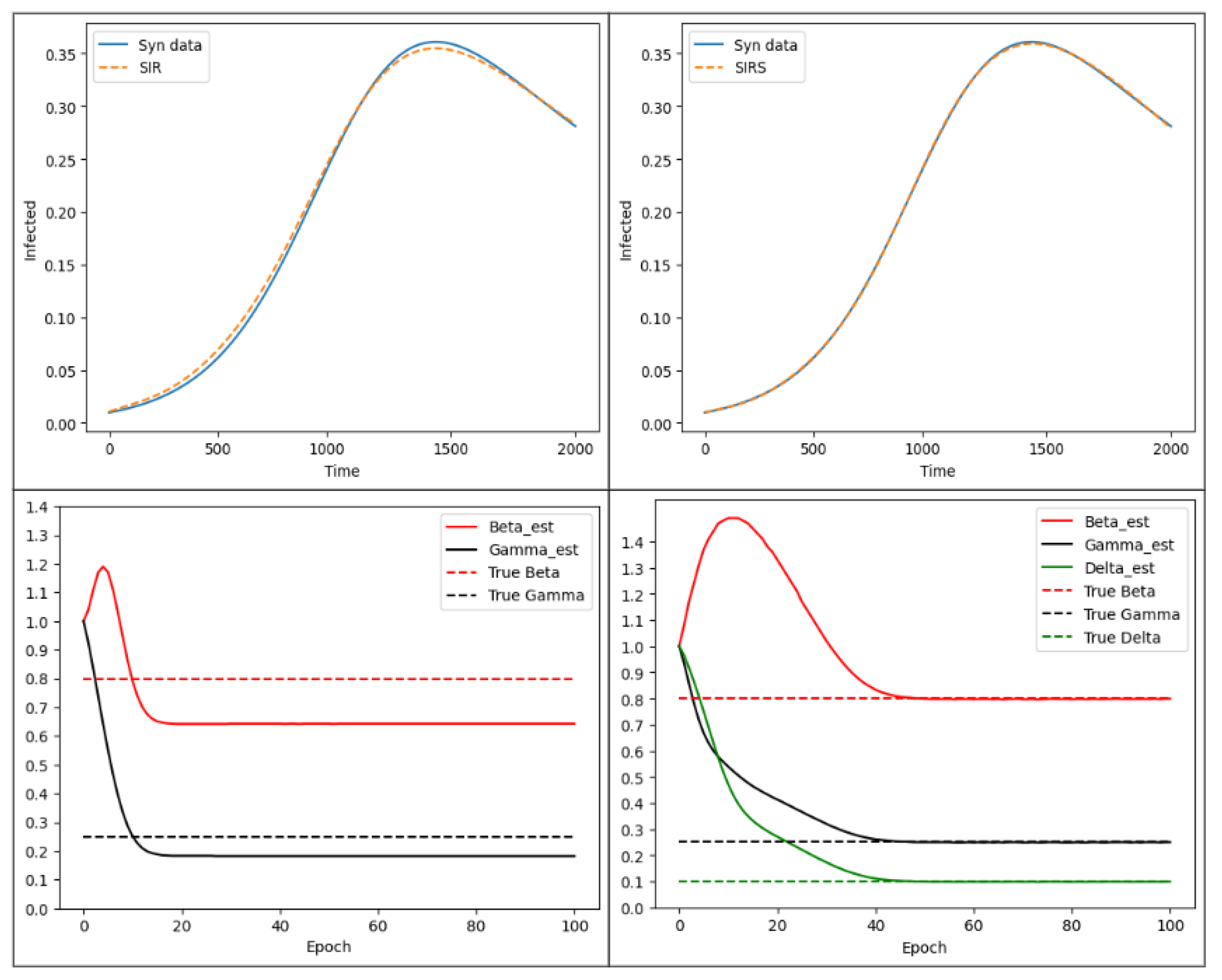
The results obtained in this experiment by the PINNs trained with the SIR model (Figure 6 top left) and the SIRS model (Figure 6 top right) show that they are able to estimate the parameters in such a way that the infected curve produced by the PINN is equal to the one measured in the network, although the infected curve generated by PINN-SIR is not exactly similar to the infected measurement made in the network. In the parameter estimation tasks, the PINN trained with the SIRS model correctly estimates the parameters (Figure 6 bottom left), while the PINN trained with the SIR model (Figure 6 bottom right) cannot estimate β or γ . The PINN trained with the SIR model took 152 s to estimate the parameters, while the PINN trained with the SIRS model took 157 s.
Finally, a comparison of the estimates from the three methods compared in this study can be seen in Table 2. The MC MSE method correctly estimates the parameters of the SIRS model while finding parameters for the SIRS model that are outside the bounds of these parameters, i.e., 0 β , γ , δ 1 . However, the MC log-square model is not able to estimate the parameters. On the other hand, PINN-SIRS identifies the parameters, while PINN-SIR is not able to estimate them, as was expected based on its training.

3.4. Discussion

In this study, we compared the performance of two methods based on Monte Carlo techniques with different loss functions and PINNs to perform the task of estimating the parameters of the propagation dynamics of malware spreading in a network. For this study, we used the SIR and SIRS models, as they have the same compartments. However, if we had only used Monte Carlo techniques we could have used any type of propagation dynamics without the limitations that PINNs impose on the input data; e.g., if the input model is a SIRS and the PINN is trained with a SIR, the ‘E’ compartment causes the PINN to make an error. We observed that in most cases both Monte Carlo methods and PINNs produced estimates very close to or even identical with the actual values. However, the PINNs had difficulty in the case described in Section 3.2, involving parameter estimation for the SIR model. In this case, both PINN-SIR and the PINN-SIRS made very good estimates of the β and γ parameters; however, the δ parameter was wrong, although it produced a result curve similar to the one measured in the network. As explained above, each simulation performed with PINN-SIRS produced a new value of δ , as this PINN is designed to produce a termination curve similar to the one it receives as input. In the case of the SIR model, both methods based on Monte Carlo techniques correctly estimated the parameters, identifying that in this case the propagation model followed by the malware in the network is a SIR model. In the experiment described in Section 3.3, the MC-MSE method correctly estimated the parameters of the SIRS model, while the MC-log-square method was unable to perform the estimation task. On the other hand, the PINNs correctly identified the parameters of the SIRS model. The computation time of these methods is a notable aspect of the comparison. The PINNs took between 140 and 160 s in both cases, depending on the estimation task, while both Monte Carlo methods took about 55 s. Although Monte Carlo methods are iterative and stochastic in nature, requiring multiple simulations to obtain reliable results, they are faster in this case. This may be because the libraries that allow neural networks to perform fast parallel computations were not compatible with the desktop we used to run the simulations. In conclusion, it is worth noting that for each malware propagation model for which the parameters need to be identified, it is necessary to have a PINN trained on that model. In contrast, with Monte Carlo-based methods it is sufficient to run one function each time a statistical inference is made in each iteration. This can be a great advantage when using computers that are not very powerful, while on newer computers the computation times will be similar due to parallel computing.
In this paper, we have compared algorithms based on Monte Carlo techniques and PINNs to solve the inverse problem in the area of malware propagation in IoT networks. However, as discussed in Section 1, studies can be found that solve the inverse problem and estimate the parameters of the ODEs. In the instance of algorithms utilizing Monte Carlo techniques, relevant research can be found in other disciplines such as physics [15] and chemistry [16], where the efficacy of these methods has been demonstrated. Nevertheless, our focus is specifically directed towards malware proliferation, as evident in our implementation of statistical inference techniques and algorithmic design, which require a rigorous theoretical basis. This comparison is infeasible because the algorithms employed to unravel the inverse problems are tailored for each specific problem. Nonetheless, we acknowledge that the Monte Carlo sampling methods are identical and the inference techniques employed are comparable. With a few adaptations in algorithm design, it can be expected that these algorithms would produce comparable accuracy. On the other hand, when comparing our work to the current state of the art, it is apparent that PINNs are utilized in numerous disciplines, including physics. However, we have identified several instances where the inverse issue is resolved for SIR models, mainly in topics related to COVID-19 [17,18]. The aforementioned works present certain advantages compared to the problem we have tackled here. In our case, we possess knowledge regarding the overall count of IoT sensors in the network, along with an estimated count of affected sensors, presuming that a number of them might be dormant or even concealed by the malware. On the other hand, research that implements PINNs in scenarios similar to COVID-19 relies on data disseminated by health institutions, which simplifies the task of PINNs in approximating the parameters [52].

4. Conclusions

The results of our comparison of the two studied methods shows that both have the potential to estimate the parameters of propagation models in a network for subsequent identification. The accuracy of both the Monte Carlo and PINN-based methods shows that their parameter estimation capabilities allow them to estimate parameters close to those used in the generation of the synthesized data. However, our numerical experiments show that each method performs better in different aspects and contexts. Therefore, the choice of the most efficient method for identifying malware propagation patterns in networks depends on the nature of the parameters to be estimated and whether the model is known or not; if it is not known, the PINN approach may have serious disadvantages. Notably, this study has several limits. In the first place, the measurements that would be carried out in a real scenario would imply that only the infected curves would be available, and these would probably be incomplete. This would certainly have an impact on the behavior of the models studied in this work for the estimation of the parameters. Furthermore, the hyperparameters of the models based on Monte Carlo techniques and PINNs were not optimized in this comparison, i.e., the same configurations were used in all experiments. Finally, in our future work we intend to develop more advanced parameter estimation methods based on the comparison presented in this paper and validate the models on real data. Building on this research, we will develop hybrid algorithms based on MC techniques and the other techniques described in the literature, e.g., least squares, maximum likelihood, etc. In addition, we will open another line of research to improve the accuracy of the PINNs in solving the inverse problem. The challenge in using both methods lies in the need for prior knowledge of the models that propagate in the network; therefore, this will be one of the main objectives of our research in our future work.

Author Contributions

Conceptualization, M.S. and R.C.-V.; methodology, M.S. and R.C.-V.; software, M.S.; validation, M.S., R.C.-V. and A.M.d.R.; formal analysis, R.C.-V. and A.M.d.R.; investigation, M.S. and R.C.-V.; resources, A.M.d.R.; data curation, M.S.; writing—original draft preparation, M.S., R.C.-V. and A.M.d.R.; writing—review and editing, M.S., R.C.-V. and A.M.d.R.; visualization, M.S.; supervision, R.C.-V. and A.M.d.R.; project administration, A.M.d.R. All authors have read and agreed to the published version of the manuscript.

Funding

This research received no external funding.

Data Availability Statement

The datasets generated and/or analyzed during the current study are available from the corresponding author on reasonable request.

Conflicts of Interest

The authors declare no conflict of interest.

References

  1. Khan, J.A.; Chowdhury, M.M. Security analysis of 5g network. In Proceedings of the 2021 IEEE International Conference on Electro Information Technology (EIT), Mt. Pleasant, NI, USA, 14–15 May 2021; pp. 001–006. [Google Scholar]
  2. Wu, H.; Han, H.; Wang, X.; Sun, S. Research on artificial intelligence enhancing internet of things security: A survey. IEEE Access 2020, 8, 153826–153848. [Google Scholar] [CrossRef]
  3. Sadhu, P.K.; Yanambaka, V.P.; Abdelgawad, A. Internet of things: Security and solutions survey. Sensors 2022, 22, 7433. [Google Scholar] [CrossRef]
  4. Clim, A.; Toma, A.; Zota, R.D.; Constantinescu, R. The Need for Cybersecurity in Industrial Revolution and Smart Cities. Sensors 2022, 23, 120. [Google Scholar] [CrossRef]
  5. Aslan, Ö.; Aktuğ, S.S.; Ozkan-Okay, M.; Yilmaz, A.A.; Akin, E. A comprehensive review of cyber security vulnerabilities, threats, attacks, and solutions. Electronics 2023, 12, 1333. [Google Scholar] [CrossRef]
  6. Mittal, M.; Kumar, K.; Behal, S. Deep learning approaches for detecting DDoS attacks: A systematic review. Soft Comput. 2023, 27, 13039–13075. [Google Scholar] [CrossRef]
  7. Victoire, T.A.; Vasuki, M.; Karunamurthy, A.; Soundarya, D.; Sarumathi, S. A Survey on Cyber Security Threats and its Impact on Society. Int. J. Res. Eng. Sci. Manag. 2023, 6, 146–152. [Google Scholar]
  8. del Rey, A.M.; Vara, R.C.; González, S.R. A computational propagation model for malware based on the SIR classic model. Neurocomputing 2022, 484, 161–171. [Google Scholar] [CrossRef]
  9. Furtado, P. Epidemiology SIR with regression, arima, and Prophet in forecasting COVID-19. Eng. Proc. 2021, 5, 52. [Google Scholar]
  10. Wong, W.; Juwono, F.H. Estimating effective reproduction number for sir compartmental model: A stochastic evolutionary approach. J. Soc. Comput. 2022, 3, 182–189. [Google Scholar] [CrossRef]
  11. Cantó, B.; Coll, C.; Sánchez, E. Estimation of parameters in a structured SIR model. Adv. Differ. Equ. 2017, 2017, 33. [Google Scholar] [CrossRef]
  12. Marinov, T.T.; Marinova, R.S.; Omojola, J.; Jackson, M. Inverse problem for coefficient identification in SIR epidemic models. Comput. Math. Appl. 2014, 67, 2218–2227. [Google Scholar] [CrossRef]
  13. Zang, W.; Zhang, P.; Zhou, C.; Guo, L. Locating multiple sources in social networks under the SIR model: A divide-and-conquer approach. J. Comput. Sci. 2015, 10, 278–287. [Google Scholar] [CrossRef]
  14. Piazzola, C.; Tamellini, L.; Tempone, R. A note on tools for prediction under uncertainty and identifiability of SIR-like dynamical systems for epidemiology. Math. Biosci. 2021, 332, 108514. [Google Scholar] [CrossRef] [PubMed]
  15. Taddy, M.A.; Lee, H.K.; Sansó, B. Fast inference for statistical inverse problems. Inverse Probl. 2009, 25, 085001. [Google Scholar] [CrossRef]
  16. da Silva, W.B.; Dutra, J.C.; Knupp, D.C.; Abreu, L.A.; Silva Neto, A.J. Estimation of timewise varying boundary heat flux via Bayesian filters and Markov Chain Monte Carlo method. In Computational Intelligence in Emerging Technologies for Engineering Applications; Springer: Cham, Switzerland, 2020; pp. 137–153. [Google Scholar]
  17. Schiassi, E.; De Florio, M.; D’Ambrosio, A.; Mortari, D.; Furfaro, R. Physics-informed neural networks and functional interpolation for data-driven parameters discovery of epidemiological compartmental models. Mathematics 2021, 9, 2069. [Google Scholar] [CrossRef]
  18. Grimm, V.; Heinlein, A.; Klawonn, A.; Lanser, M.; Weber, J. Estimating the time-dependent contact rate of SIR and SEIR models in mathematical epidemiology using physics-informed neural networks. Electron. Trans. Numer. Anal. 2022, 56, 1–27. [Google Scholar] [CrossRef]
  19. Ferrández, M.R.; Ivorra, B.; Redondo, J.L.; Ramos del Olmo, Á.M.; Ortigosa, P.M. A multi-objective approach to estimate parameters of compartmental epidemiological models. Application to Ebola Virus Disease epidemics. Ene 2021, 12, 42. [Google Scholar]
  20. Shandilya, S.K.; Upadhyay, S.; Kumar, A.; Nagar, A.K. AI-assisted Computer Network Operations testbed for Nature-Inspired Cyber Security based adaptive defense simulation and analysis. Future Gener. Comput. Syst. 2022, 127, 297–308. [Google Scholar] [CrossRef]
  21. Barlas, Y. Formal aspects of model validity and validation in system dynamics. Syst. Dyn. Rev. J. Syst. Dyn. Soc. 1996, 12, 183–210. [Google Scholar] [CrossRef]
  22. Lee, G.; Kim, W.; Oh, H.; Youn, B.D.; Kim, N.H. Review of statistical model calibration and validation—from the perspective of uncertainty structures. Struct. Multidiscip. Optim. 2019, 60, 1619–1644. [Google Scholar] [CrossRef]
  23. Savage, L.J. The Foundations of Statistics; Courier Corporation: New York, NY, USA, 1972. [Google Scholar]
  24. Bar-Yam, Y. Dynamics of Complex Systems; CRC Press: Boca Raton, FL, USA, 2019. [Google Scholar]
  25. Mingers, J. A critique of statistical modelling in management science from a critical realist perspective: Its role within multimethodology. J. Oper. Res. Soc. 2006, 57, 202–219. [Google Scholar] [CrossRef]
  26. Kaniadakis, G.; Baldi, M.M.; Deisboeck, T.S.; Grisolia, G.; Hristopulos, D.T.; Scarfone, A.M.; Sparavigna, A.; Wada, T.; Lucia, U. The κ-statistics approach to epidemiology. Sci. Rep. 2020, 10, 19949. [Google Scholar] [CrossRef] [PubMed]
  27. Andrade, J.; Duggan, J. An evaluation of Hamiltonian Monte Carlo performance to calibrate age-structured compartmental SEIR models to incidence data. Epidemics 2020, 33, 100415. [Google Scholar] [CrossRef] [PubMed]
  28. Hattaf, K.; Yousfi, N.; Tridane, A. Mathematical analysis of a virus dynamics model with general incidence rate and cure rate. Nonlinear Anal. Real World Appl. 2012, 13, 1866–1872. [Google Scholar] [CrossRef]
  29. Miao, H.; Xia, X.; Perelson, A.S.; Wu, H. On identifiability of nonlinear ODE models and applications in viral dynamics. SIAM Rev. 2011, 53, 3–39. [Google Scholar] [CrossRef]
  30. Figueira, A.; Vaz, B. Survey on synthetic data generation, evaluation methods and GANs. Mathematics 2022, 10, 2733. [Google Scholar] [CrossRef]
  31. Diekmann, O.; Heesterbeek, J.A.P. Mathematical Epidemiology of Infectious Diseases: Model Building, Analysis and Interpretation; John Wiley & Sons: Hoboken, NJ, USA, 2000; Volume 5. [Google Scholar]
  32. Brauer, F.; Van den Driessche, P.; Wu, J.; Allen, L.J. Mathematical Epidemiology; Springer: Berlin/Heidelberg, Germany, 2008; Volume 1945. [Google Scholar]
  33. Kwok, K.O.; Tang, A.; Wei, V.W.; Park, W.H.; Yeoh, E.K.; Riley, S. Epidemic models of contact tracing: Systematic review of transmission studies of severe acute respiratory syndrome and middle east respiratory syndrome. Comput. Struct. Biotechnol. J. 2019, 17, 186–194. [Google Scholar] [CrossRef]
  34. del Rey, A.M. Mathematical modeling of the propagation of malware: A review. Secur. Commun. Netw. 2015, 8, 2561–2579. [Google Scholar] [CrossRef]
  35. Reis, W.P.N.d.; Silva, G.J.d.; Junior, O.M.; Vivaldini, K.C.T. An extended analysis on tuning the parameters of Adaptive Monte Carlo Localization ROS package in an automated guided vehicle. Int. J. Adv. Manuf. Technol. 2021, 117, 1975–1995. [Google Scholar] [CrossRef]
  36. Driggers, J.C.; Vitale, S.; Lundgren, A.; Evans, M.; Kawabe, K.; Dwyer, S.; Izumi, K.; Schofield, R.; Effler, A.; Sigg, D.; et al. Improving astrophysical parameter estimation via offline noise subtraction for Advanced LIGO. Phys. Rev. D 2019, 99, 042001. [Google Scholar] [CrossRef]
  37. Reis, M.d.; Yang, Z. Approximate likelihood calculation on a phylogeny for Bayesian estimation of divergence times. Mol. Biol. Evol. 2011, 28, 2161–2172. [Google Scholar] [CrossRef] [PubMed]
  38. Kanaan, M.; Farrington, C. Matrix models for childhood infections: A Bayesian approach with applications to rubella and mumps. Epidemiol. Infect. 2005, 133, 1009–1021. [Google Scholar] [CrossRef] [PubMed]
  39. Dangerfield, B.; Duggan, J. Optimization of system dynamics models. In System Dynamics: Theory and Applications; Springer: New York, NY, USA, 2020; pp. 139–152. [Google Scholar]
  40. Raissi, M.; Perdikaris, P.; Karniadakis, G.E. Physics-informed neural networks: A deep learning framework for solving forward and inverse problems involving nonlinear partial differential equations. J. Comput. Phys. 2019, 378, 686–707. [Google Scholar] [CrossRef]
  41. Berkhahn, S.; Ehrhardt, M. A physics-informed neural network to model COVID-19 infection and hospitalization scenarios. Adv. Contin. Discret. Model. 2022, 2022, 61. [Google Scholar] [CrossRef] [PubMed]
  42. Tartakovsky, A.M.; Marrero, C.O.; Perdikaris, P.; Tartakovsky, G.D.; Barajas-Solano, D. Physics-informed deep neural networks for learning parameters and constitutive relationships in subsurface flow problems. Water Resour. Res. 2020, 56, e2019WR026731. [Google Scholar] [CrossRef]
  43. Jiang, X.; Wang, D.; Chen, X.; Zhang, M. Physics-Informed Neural Network for Optical Fiber Parameter Estimation From the Nonlinear Schrödinger Equation. J. Light. Technol. 2022, 40, 7095–7105. [Google Scholar] [CrossRef]
  44. Zhao, S.; Peng, Y.; Zhang, Y.; Wang, H. Parameter estimation of power electronic converters with physics-informed machine learning. IEEE Trans. Power Electron. 2022, 37, 11567–11578. [Google Scholar] [CrossRef]
  45. Robert, C.P.; Casella, G.; Casella, G. Introducing Monte Carlo Methods with r; Springer: Berlin/Heidelberg, Germany, 2010; Volume 18. [Google Scholar]
  46. Jin, Y.F.; Yin, Z.Y.; Zhou, W.H.; Horpibulsuk, S. Identifying parameters of advanced soil models using an enhanced transitional Markov chain Monte Carlo method. Acta Geotech. 2019, 14, 1925–1947. [Google Scholar] [CrossRef]
  47. Durmus, A.; Moulines, É.; Pereyra, M. A Proximal Markov Chain Monte Carlo Method for Bayesian Inference in Imaging Inverse Problems: When Langevin Meets Moreau. SIAM Rev. 2022, 64, 991–1028. [Google Scholar] [CrossRef]
  48. Hornik, K.; Stinchcombe, M.; White, H. Multilayer feedforward networks are universal approximators. Neural Netw. 1989, 2, 359–366. [Google Scholar] [CrossRef]
  49. Baydin, A.G.; Pearlmutter, B.A.; Radul, A.A.; Siskind, J.M. Automatic differentiation in machine learning: A survey. J. Marchine Learn. Res. 2018, 18, 1–43. [Google Scholar]
  50. Kermack, W.O.; McKendrick, A.G. A contribution to the mathematical theory of epidemics. Proc. R. Soc. Lond. Ser. Contain. Pap. Math. Phys. Character 1927, 115, 700–721. [Google Scholar]
  51. Lu, L.; Meng, X.; Mao, Z.; Karniadakis, G.E. DeepXDE: A deep learning library for solving differential equations. SIAM Rev. 2021, 63, 208–228. [Google Scholar] [CrossRef]
  52. Heldmann, F.; Berkhahn, S.; Ehrhardt, M.; Klamroth, K. PINN training using biobjective optimization: The trade-off between data loss and residual loss. J. Comput. Phys. 2023, 488, 112211. [Google Scholar] [CrossRef]
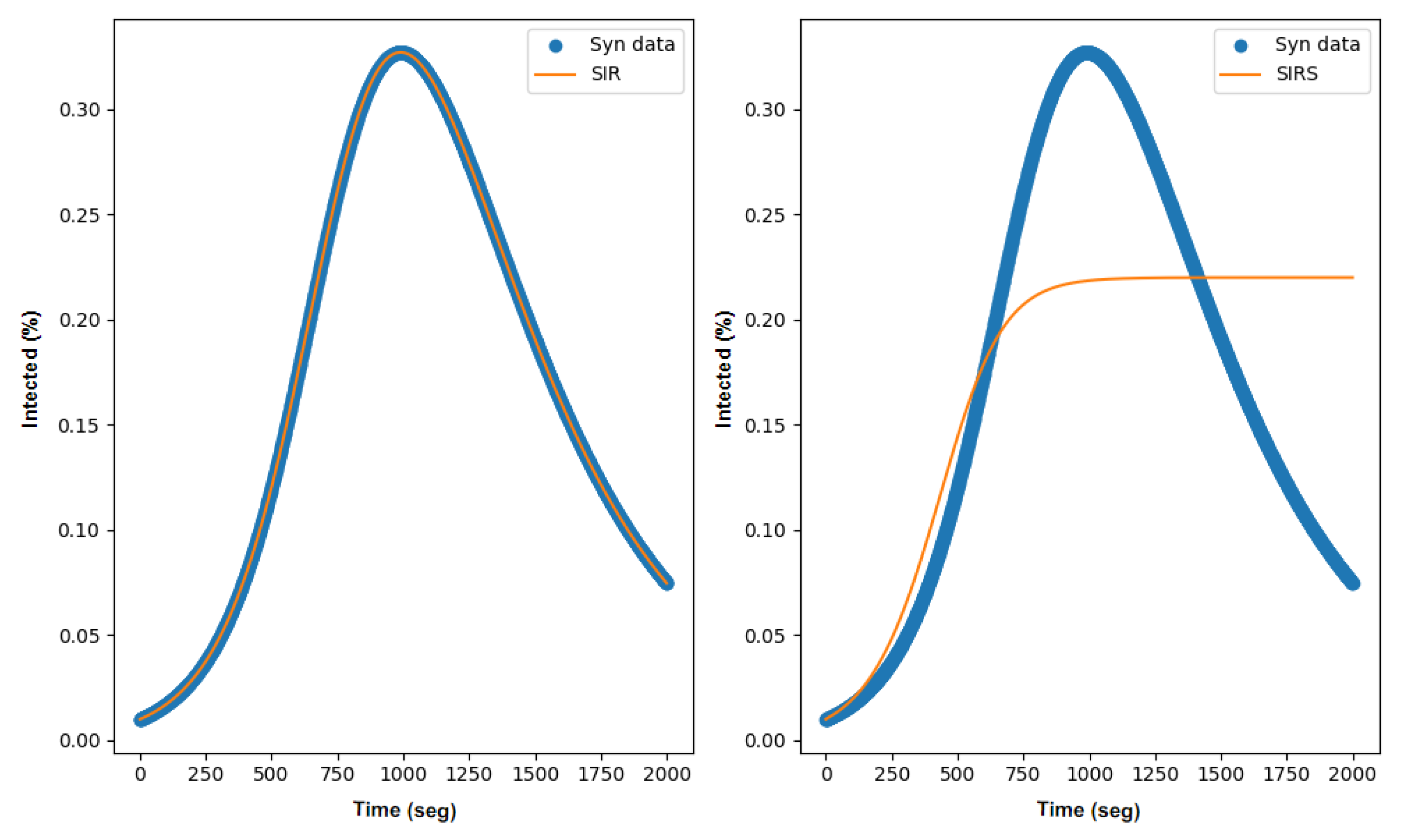
Figure 1. Data generated synthetically according to the SIR model with parameters β = 0.8 and γ = 0.25 (blue). Data were generated using parameters calculated using the Monte Carlo MSE loss function method for the SIR model and SIRS model (orange).
Technologies 11 00133 g001
Figure 2. Data generated synthetically according to the SIR model with parameters β = 0.8 and γ = 0.25 (blue). Data were generated using parameters calculated using the Monte Carlo log-square loss function method for the SIR model and SIRS model (orange).
Technologies 11 00133 g002
Figure 3. Top: data synthetically generated according to the SIR model with parameters beta = 0.8 and gamma = 0.25 (blue). Data were created with the parameters calculated by the PINN for the SIR model and SIRS model (orange). Bottom: parameters estimated by the PINNs trained with the SIR model (left) and SIRS model (right).
Technologies 11 00133 g003
Figure 4. Data generated synthetically according to the SIRS model with parameters β = 0.8 , γ = 0.25 and δ = 0.1 (blue). Data were generated using parameters calculated using the Monte Carlo MSE loss function method for the SIR model and SIRS model (orange).
Technologies 11 00133 g004
Figure 5. Data generated synthetically according to the SIRS model with parameters β = 0.8 , γ = 0.25 and δ = 0.1 (blue). Data were generated using parameters calculated using the Monte Carlo MSE loss function method for the SIR model and SIRS model (orange).
Technologies 11 00133 g005
Figure 6. Top: data synthetically generated according to the SIRS model with parameters beta = 0.8 and gamma = 0.25 (blue). Data were created with the parameters calculated with a PINN for the SIR model and SIRS model (orange). Bottom: parameters estimated by the PINNs trained with the SIR model (left) and SIRS model (right).
Technologies 11 00133 g006
Table 1. Estimated SIR and SIRS model parameters were obtained by each compared method. Highlighted in red are the values that cannot be taken by the parameters since they are bounded 0 β , γ , δ 1 .
MethodSIRSIRS
MC MSE β = 0.8 β = −1.49
γ = 0.25 γ = −1.49
δ = 1.46
MC Log Square β = 0.8 β = −18.71
γ = 0.25 γ = −18.71
δ = 18.69
PINN β = 0.8 β = 0.8
γ = 0.25 γ = 0.25
δ = 5.4 × 10 4
Table 2. Estimated SIR and SIRS model parameters were obtained by each compared method. Highlighted in red are the values that cannot be taken by the parameters since they are bounded 0 β , γ , δ 1 .
MethodSIRSIRS
MC MSE β = 0.7 β = 0.8
γ = 0.187 γ = 0.25
δ = 0.1
MC Log Square β = 0.7 β = 1.9
γ = 0.18 γ = 1.22
δ = 5.83
PINN β = 0.7 β = 0.8
γ = 0.187 γ = 0.25
δ = 0.1
Disclaimer/Publisher’s Note: The statements, opinions and data contained in all publications are solely those of the individual author(s) and contributor(s) and not of MDPI and/or the editor(s). MDPI and/or the editor(s) disclaim responsibility for any injury to people or property resulting from any ideas, methods, instructions or products referred to in the content.