Optimization of the Pick-Up and Delivery Technology in a Selected Company: A Case Study

Abstract

This article deals with pick-up and delivery activities in a selected company that focuses on the distribution of products in the gastronomic sector of the market and suggests how to make the present approach more efficient. The introductory part of the article clarifies the meanings of basic concepts related to the issue of optimizing the logistics processes in the company. The crucial goal is to analyze the existing pick-up and delivery technology and then, in the application part of the article, to propose adequate measures in the context of streamlining these activities with their technical and economic evaluation. An analysis of current delivery routes, which are used for the distribution of gastronomic products, is first performed. Thereafter, the routes are optimized with the aim of minimizing the total distance traveled by using the Operations Research methods, namely: the Hungarian method, Vogel approximation method, nearest neighbor method and the Routin route planner which is based on a principle of the Greedy algorithm. At the end of the article, a technical and economical evaluation of the findings is discussed, wherein the individual results of optimization through selected methods are first compared and then, new optimized routes are selected.

1. Introduction

By optimizing pick-up and delivery routes of various transport-logistics companies, when using the methods of Operations Research, it is possible to reduce transport costs and other attributes for operating such routes. The savings in transport performance or fuel consumption may not be significant in the short term (one transport or one day), but, e.g., in a one-year period, the value of savings could be remarkable. The saved values could be used, for example, for other transport performance, reinvesting in company development, marketing and so forth.

This article deals with the analysis of the current pick-up and delivery activity in a selected company that deals with the distribution of gastronomic equipment. After this analysis, the optimization of current pick-up routes is performed by methods of operation research. There are three selected and applied methods: the Hungarian method, Vogel approximation method, the nearest neighbor method and the Routin route planner. The individual results after the optimization of the initial routes are compared with each other and, on the basis of this comparison, new pick-up routes with an adjusted order of unloading points are recommended to the selected company. These recommendations are supplemented by a technical and economical evaluation of the results, where the potential saving in transport performance, which represents an optimization criterion, and saving in fuel consumption costs are calculated after the application of the proposed route modification. Thus, the objective of this research is to define optimal delivery routes in terms of supplying predetermined customers when minimizing the total distance traveled.

The optimization of specific pick-up and delivery routes of the distribution enterprise when using multiple Operations Research methods as well as a selected web application along with a technical and economical evaluation of the final outcomes is where the novelty of our research lies. Based on a literature review in the following section of the manuscript, it was found that no similar scientific work when using identical vehicle routing problem methods to those applied in this manuscript has been published yet. Hence, our research clearly contributes to the gaps in the existing literature.

2. Literature Review

The optimization of transport networks, among others, includes addressing the distribution tasks—pick-up and delivery problem—using mathematical (Operations Research) methods. According to Cheng [1], Hamiltonian circuits have a crucial role in terms of optimization tasks, especially in addressing distribution tasks where each vertex (customer, supplier, logistics center and so forth) needs to be visited just once. To address this problem, a number of conditions have been defined that the graph must adhere to including the Hamiltonian circuit [2]. These days, optimization in transport networks has many options to use and can save considerable resources. This is the case in both the corporate sphere, where the goal is to optimize the distribution cost and transport network operation, and in the personal sphere, where the emphasis is placed on searching for the shortest possible route from point A to point B.

As described by numerous authors in a variety of publications, e.g., [3,4,5,6,7,8,9], in practice, many different distribution systems are utilized. All of the below methods were taken into account as potential tools for the optimization purpose, however, due to specific input conditions set in this research, only some of them can be deemed as adequate (see Section 3.1):

• Gradual distribution (intermediate warehousing)—each stage represents placement of a product in a warehouse. It is a system in which warehouses are used to a maximum extent. Distribution centers completing sales requirements are typical examples of such a distribution.
• Direct delivery system—products are delivered to the point of consumption directly from one or more storage locations, or directly from the production factory. The supplier has at his disposal one central warehouse to which he collects individual consignments, and from which he also handles them. This system includes cross-dock operations as well, which are mainly applied to high-volume product flows towards the retail network. The distribution center is integrated directly into the chain segment between a larger number of suppliers on one side and a retail network on another. Deliveries from all suppliers are collected to this center, stored in appropriate warehouse departments, and completed (assembled) according to retail network requirements. Consequently, the delivery itself is usually carried out at an exact time.
• Combined systems—the combination of the previous two systems is most commonly used. It determines which products will be distributed directly and which through intermediate warehousing. These systems also make it possible to deliver supplies in an alternative way.
• Postponement strategies for final operations—modern distribution systems do not only wait for the final order, but are also based on forecasting. This is also related to the risk that actual orders will differ from those anticipated. If some production distribution operations can be postponed until a specific order arrives, this risk can be substantially reduced. The basis is to keep the products in the production process in the unfinished state for as long as possible and to make the final adjustment up to confirming the customer order. The main effect of this process is to reduce the product range in stock, minimize the risk of poor inventory location and make better utilization of storage capacity for completing operations [10].
• Coupling methods—these are carried out due to an effort to cut down shipping cost. The larger the shipment, the lower the shipping cost per unit. Coupling also improves shipping cost control.

The optimal distribution concept consists in the optimal number of locations, combination of own and contracted warehouses, appropriate ratio of in-house and external transport—outsourcing, including a method of planning and management—and all of these while complying with capacity and customer requirements, and minimum costs. The distribution efficiency is affected by the geographical distribution of the partners (stakeholders) involved in the distribution process. It considerably affects the level of customer service and distribution cost.

The concept of distribution and distribution systems is undoubtedly related to pick-up and delivery tasks. In most models, the pick-up and delivery of shipments from the logistics center (LC)—often referred to as the “first and last mile” of the entire transport chain—in terms of the issue of city logistics are provided by road carriers with their own vehicles. The only exception is those shipments that are delivered directly to the recipient’s own railway siding or to public reloading tracks at the destination station by the system of preferential or ordinary train formation [11,12].

Pick-up and delivery technology should be managed according to the following principles, as described in [13]:

• consistent operational management according to the current needs of the network and contracted transport volumes; i.e., exact transport requirements will be assigned to a road carrier in a short-term period, within a long-term contracted capacity;
• the principle of maximum utilization of road vehicles, which leads to maximum profitability of transport;
• providing transport services directly from home to home by the relevant regional road carrier, direct contact with the customer, delivery of shipment and shipping documents are highly desirable;
• effort to minimize handling cost to a maximum extent; i.e., using appropriate transshipment mechanisms in an LC, prompt cargo transshipment to the customer with respect to an option of using a vehicle for further carriage;
• distribution by railways only when delivering (or dispatching) to the recipient’s own siding or to public reloading tracks at the destination station, i.e., without reloading and other logistics operations in relevant LC.

As presented by Karakikes et al., the implementation of appropriate mechanisms for the management of technological processes and quality of services is a key element to operate the LC on its own in the context of pick-up and delivery tasks, which means [14]:

• tracking shipments on international and domestic routes;
• monitoring of technological processes in the LC;
• monitoring of road vehicles during collection and distribution;
• checking the collection of load and transition between routes;
• operational planning of capacities, means of transport, routes and operation of LCs and the network as a whole;
• evidence of vehicles, wagons, containers and other means, tracking the movement of means of transport in LCs, in the network, to customers;
• addressing deviations from the plan and extraordinary traffic;
• service quality management, i.e., just-in-time delivery, timeliness delivery, accuracy, flexibility and reliability;
• providing transport and logistics services;
• dispatching management of the LC and the network as a whole.

Planning the pick-up and delivery of shipments as well as the movement of means of transport to the customer or to intermediate warehouses must be optimized in real time depending on various criteria (such as cost, distance traveled, empty journeys, etc.), as stated by the authors Graf and Stadlmann [15], and Masuda et al. [16]. This service should be designed so that the final customer does not have to be equipped with appropriate handling equipment for reloading the shipment.

As an extension to our research topic, Musollino et al. in [17] present the integration of the Mansky paradigm principle as path choice problem and general vehicle routing problem tools when applying methodological and experimentation approaches; i.e., an analysis of similarity of criteria to create various alternatives for distribution routes and creating a choice route model regarding freight vehicles. Similarly, even in [18], Croce et al. deal with a path choice problem and vehicle routing problem specifically in the Calabria region (southern Italy) in order to compare specific delivery routes with simulated and optimized routes of commercial vehicles with an aim to assess the similarity and coverage levels.

In addition to the vehicle routing problem, specific approaches based on network theory and game theory in regard to a distribution problem could also be considered. For instance, Arena et al. discuss the Parrondo paradox concerning the role of chaos when proving that two separate losing games can be combined following a random or periodic strategy to have a resulting winning game [19]. In analogy, Guanhui focuses on analyzing various game theory models, particularly in the supply chain. The author suggests a multi-enterprise output game theory approach under the circumstances of information asymmetry from the point of view of function, hypothesis parameters and modeling basis, and evaluates the impact of producer’s output adjustment speed attributes on the entire supply chain [20].

3. Methodology of the Addressed Problem

Operations Research is a multidisciplinary subject that combines knowledge, experience and skills from different industries. The advantage of the Operations Research methods lies in their wide use to address problems of varying complexity. Operations Research can be viewed as a scientific discipline that includes a wider range of scientific subdisciplines focused on analyzing and managing activities in terms of addressing decision-making problems. These areas of Operations Research can be used in decision-making problems themselves, but also as a combination of several of them [21].

The aim of Operations Research is to set up operations and their interconnections so that the examined system is as effective as possible. Effectiveness must be assessed on the basis of objective or subjective criteria. A mathematical or physical model of a system is often created in order to perform tests of its functionality [21]. Section 3.1 describes the selected research methods in more detail.

3.1. Research Methods

Considering the issue addressed, its scale, transport territory, all the input conditions and other possible aspects and intricacies, it was decided by the authors as well as a panel of experts dealing with the issue of vehicle routing problems that three mathematical instruments will be applied to optimize the distribution problem.

The Hungarian method is a combinatorial optimization algorithm, which falls into special methods for addressing assignment transport problems. It was invented by the Hungarian author Egervary and belongs to the most effective methods of addressing transport problems. It is also referred to as the Kuhn–Munkres algorithm. The advantage of the Hungarian method is mainly its universality due to its use in assignment problems or vehicle routing problems, and it is also universally applicable for several types of matrices. The disadvantage of this method is relatively long computational time [21].

Several suppliers operate in the system and import various goods at different points of consumption. When suppliers accomplish their task, they return their vehicle back to the origin point. A supplier only visits the site once. The goal of this problem is to minimize the total distance traveled as much as possible. Due to these conditions, the optimal order of vertices to be operated by suppliers is compiled. In order to solve the task by the Hungarian method, the following conditions must be met [22]:

• equality of the number of rows and columns (symmetric distance matrix); if this condition is not met, it is necessary to add a fictitious row with prohibitive rates (when minimizing, values are to be higher than the highest value of the distance matrix, when maximizing, we assign the value of 0);
• the distance matrix must be quantifiable;
• suppliers’ capacities and customers’ requirements must be homogeneous (any customer can be served by any supplier).

The procedure is given as follows [21]:

• Step 1. Listing distances—compilation of the distance matrix.
• Step 2. Row reduction—select the lowest value in each row; this value is then subtracted in individual rows, and this step gives us the required zeros in each row. This step is not repeated in the calculation process.
• Step 3. Column reduction—this step is similar to the second step, except that the lowest number is now selected in each column and subtracted from the given values in a particular column.
• Step 4. Placement of cross rows—in this step, the independent zeros that are individually in a column or row are identified. They are marked (crossed out) by either vertical or horizontal rows to use as few crossed rows as possible.
• Step 5. Modifying a matrix and selection of a minimum value—in the matrix, non-crossed numbers are searched and the number with the lowest value is identified. This number is designated as, for example, the letter n. Values of numbers that are crossed out once do not change. Numbers that are crossed out twice are increased by a value of n. From numbers that are not crossed out, the value of n is subtracted.
• Step 6. Finding a path—in the matrix, zero-value cells are nodes. A path can pass through this place provided that the shortest path is met. Here, it applies that it is possible to pass through each site only once. The aim is to pass through all the sites so that the circuit distance is as short as possible. As a result, the route starts at site number 1 and ends at site number 1.
• Step 7. Final procedure—repeat Steps 4 and 5 until the final solution is reached. The end of the calculation process occurs at the moment of closing the entire circuit, where the route leads through all the sites. Steps 4 and 5 are carried out together, this is called iteration. After modifying the matrix by Step 5, we obtain the first iteration.
• Step 8. Route distance calculation—the calculation is based on the first unmodified matrix in which we write the distances of each route. Here, we indicate the individual values that result from the assigned route. The values are summed and the final circuit distance is calculated.

Following the abovementioned steps, it can be stated that even the Hungarian method is suitable to be applied for addressing the objective of this publication, due to its appropriateness for scenarios where one or multiple suppliers serve more customers or are operated by several other suppliers to travel over short or longer distances among each other as well as the necessity to have balanced distribution tasks.

The Vogel approximation method (hereinafter VAM) is an approximation method used to deal with transport problems and is a member of the distribution tasks that fall into the tasks of linear programming. This method is one of the most widely used approximate methods by which transport problems are usually solved. Its main advantage lies in the fact that even for large-scale tasks, its results are very close to the optimum and its procedure is not time-consuming [22].

According to [23], the VAM is an improved version of the least cost method and the northwest corner method. In its general procedure, better initial basic feasible solutions, which are understood as basic feasible solutions that report a smaller value in the objective (minimization) function of a balanced transport problem (sum of the supply = sum of the demand), are obtained. The Vogel approximation method is also called the penalty method because the difference costs chosen are nothing but the penalties of not choosing the least cost routes. It consists in an iterative approach that can be used to address a single-circuit transport problem. The procedure of using the Vogel approximation method is as follows [22]:

• Step 1. The basic element of this method is to compile a default symmetric (balanced) distance table among individual locations of one circuit route.
• Step 2. For each row and column of a default distance table, it is necessary to calculate the difference between the two lowest values. The difference value is written on the table’s right side for rows and at the bottom for columns.
• Step 3. The highest possible value of all the difference values is then selected. For the row or column with the highest difference value, the lowest value in the distance table is identified. This value represents the first segment of the circuit and presents the order in which the circuit will be operated.
• Step 4. Both the row and the column for the selected value must be removed (crossed out). Furthermore, it is imperative to remove a value which, with the value currently occupied, could close the circuit route without operating all the necessary locations.
• Step 5. The next step is to recalculate the differences for the remaining rows and columns, followed by the same procedure as for Step 3.
• Step 6. We repeat the above procedure until all the necessary locations are ranked in one circuit route.

This method is suitable for models where one or multiple operators distribute cargo to multiple customers (i.e., delivery tasks) or there are several other operators (i.e., pick-up tasks) over shorter or longer distances traveled. Furthermore, each transport problem dealing with determination of the optimal transport plan by this method needs to be balanced, i.e., requirements of the destination sites must be equal to source capacities and, besides that, all the capacities and requirements must be depleted. On the basis of the aforesaid reasons, it is appropriate to apply the Vogel approximation method for the purpose of this work.

The nearest neighbor method is considered one of the simplest heuristic methods for addressing routing transport problems. It was decided to apply this algorithm due to the fact that it is suitable for types of tasks where only one supplier collects or delivers products to predetermined locations even in urban or suburban territory. After passing through all the planned stops (vertices), the vehicle returns to the point of origin. Each vertex can only be visited once. The aim of this method is to help find a solution specifying the optimal operation order of individual locations while minimizing the distance traveled or total shipping cost. This heuristic method is a simple technique and does not need more complicated calculations. The data source consists of a distance matrix among individual vertices, which is searched sequentially [22,24].

According to formulations written in a research study [25], this algorithm is one of the effective methods used to address a vehicle routing problem. The principle of the nearest neighbor algorithm starts by choosing an origin point from which the most advantageous connection to another point is to be found, and this procedure is applied until all the defined vertices are visited (operated). Once we connect all the vertices, we will return to the origin point. This method’s algorithm is summarized in the following steps [25]:

• Step 1. Identify a point of origin and, in the distance matrix, the column corresponding to the given location is marked (crossed).
• Step 2. Seek a row corresponding to the given location and, in that row, find the field with a minimum value, and thereby another place to visit is determined.
• Step 3. Find a column with this new location and cross it. Search for a row corresponding to the given location and, in that row, find the field with the minimum value; thus, apply Steps 2 and 3 until all the columns are crossed out.
• Step 4. In the last row, occupy the field in a column corresponding to an origin point, so the whole circuit is actually closed.
• Step 5. Select another location as an origin point and, applying Steps 2–5, define the circuit route for this origin point.

As stated in [24], in the distance matrix with n vertices, we come to a situation where we have n circuit routes and, from these routes, the best one needs to be determined, i.e., the one with the lowest sum of values. If the task has an asymmetric distance matrix, it is also necessary to find a “backward” route for each location, either by crossing (marking) the rows, and then searching for the minimum values in the relevant columns, or by converting the original matrix to transposed type, and then applying the original procedure to it.

Following the previously mentioned statements, the nearest neighbor method appears to be perfectly suitable in terms of its application for the objective of this research work, i.e., to specify optimal delivery routes to operate defined unloading points when minimizing distance traveled.

3.2. Presentation of the Addressed Problem

The issue addressed is based on the need to optimize the already existing delivery routes of the presented company at the branch in the city of České Budějovice, Czech Republic. This branch distributes gastronomic equipment throughout the year on optimized routes with the full utilization capacity of service vehicles [26]. However, the problem arises during the main season, when the seasonal demand of the operators of camps and restaurant facilities increases for the regular served customers, mainly due to the increased tourist traffic. This demand lasts only for a certain part of the year, from March to November. Due to the increased demand, the company does not have enough standard delivery routes to operate given locations, so it gains brigade strength for this period and introduces special seasonal delivery to customers with whom the company has a collective agreement during the main season. To cover the mentioned seasonal demand, a collective agreement with customers is used, which guarantees them delivery of the same amount of ordered goods three times a week. Thus, delivery days are set to Monday, Tuesday, Thursday and Friday, when the company delivers goods to customers in the main season. In this way, 3 routes A, B, C are operated including a total of 32 unloading points, which have not been optimized yet using adequate methods. The initial operation order of the unloading points on the selected routes is based only on the experience of the company’s employees.

Traffic in České Budějovice (congestions, lower travel speed, etc.) has a significant effect on the driving time of the delivery vehicle(s), however, given that all the defined unloading points are located near small towns outside the agglomeration of larger cities, it was not necessary to take into account the urban traffic. The journey of a delivery vehicle traveling along a part of the route leading in the extra-urban area (i.e., extra-urban part of the route) exceeds the journey of such a vehicle along the part of the same route leading in the urban area (i.e., urban part of the route) by several times in terms of kilometers traveled and time consumed. Any delay of the delivery vehicle in city traffic is therefore negligible for the purposes of this case study and was not further included in the application of single mathematical methods.

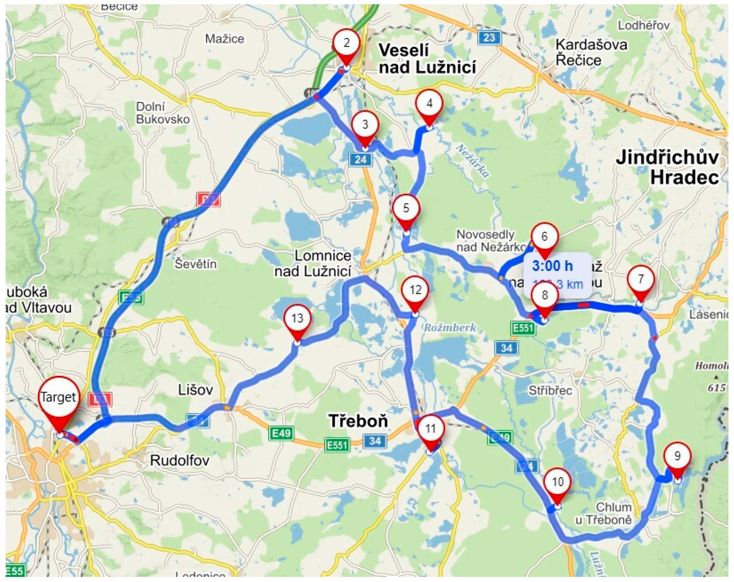
3.2.1. Default State: Route A

Route A serves 12 unloading points and is focused on serving the area northeast of České Budějovice. The following Figure 1 shows the default route A before optimization.

Table 1. Route A—default state.

Number of Unloading Points	12
Length of the route	166.6 km
Average speed	47.2 km/h
Driving time	3 h 32 min
Average time spent at a stop	8 min
Preparation and loading of goods	50 min
Total route time	5 h 58 min

shows basic data about route A.

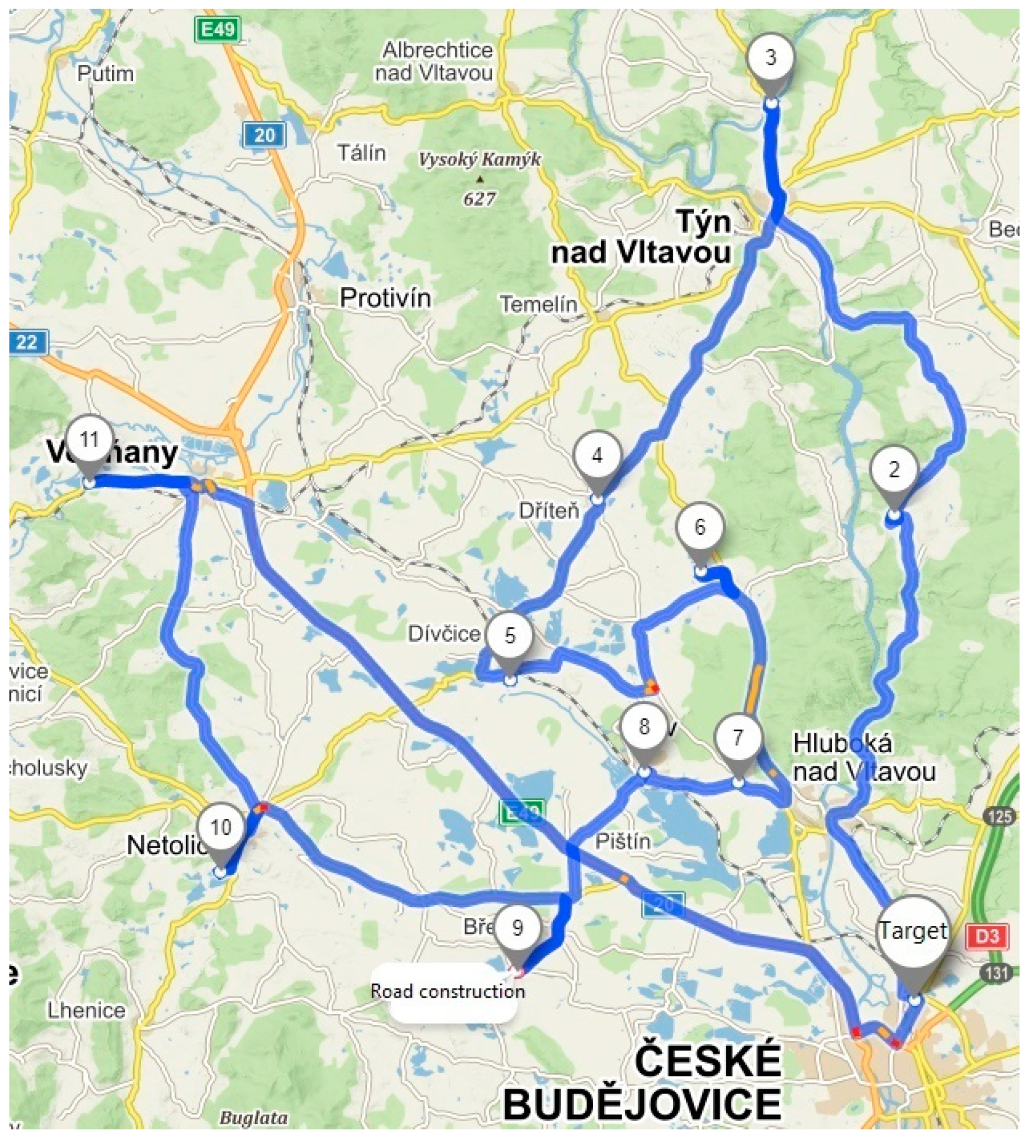
3.2.2. Default State: Route B

Route B serves 10 unloading points and is focused on serving the area south of České Budějovice. The following Figure 2 shows the default route B before optimization.

Table 2. Route B—default state.

Number of Unloading Points	10
Length of the route	181.2 km
Average speed	49.2 km/h
Driving time	3 h 41 min
Average time spent at a stop	12 min
Preparation and loading of goods	42 min
Total route time	6 h 10 min

presents basic information about this route.

3.2.3. Default State: Route C

Route C serves 10 unloading points and is focused on serving the area northwest of České Budějovice. The following Figure 3 shows the default route C before optimization.

Table 3. Route C—default state.

Number of Unloading Points	10
Length of the route	166.2 km
Average speed	46.2 km/h
Driving time	3 h 36 min
Average time spent at a stop	8 min
Preparation and loading of goods	42 min
Total route time	5 h 38 min

summarizes basic information about this route.

4. Optimization of the Pick-Up Technology

All the abovementioned methods are gradually used to optimize pick-up routes. In addition, to compare the quality of the results, the individual routes are optimized using the mobile application Routin: Smart Route Planner (hereinafter referred to as Routin), which is freely available on Google Play.

• Creating default matrices

For each path individually, first, it is necessary to build the default matrices. This matrix is formed so that for each individual unloading point on each route it is necessary to separately measure the distance and travel time from that point to each other point on the same route [27].

• Default matrix: Route A

For route A, it is necessary to create a default matrix for a total of 13 unloading points, including the company’s headquarters. In total, it is necessary to make 78 separate measurements of distances between two points to create the following

Table 4. Route A—default matrix of times and distances.

Unloading Points		A1	A2	A3	A4	A5	A6	A7	A8	A9	A10	A11	A12	A13
Sving	A1		29.7	31.6	36.6	27.1	39.8	38	31.9	44.3	33.1	25	29.3	17.5
Penzion Veselí nad Lužnicí	A2	19		6.7	7.2	17.4	27.6	31.7	25.6	44.9	33.7	25.9	18.2	21.2
Kemp Vlkov	A3	20	7		5.6	11.3	21.6	25.7	19.6	38.9	27.6	19.9	12.2	15.2
Kemp Hamr	A4	28	9	11		7.1	19.7	36.6	17.7	44.4	33.2	25.5	17.8	20.7
Penzion Klec	A5	30	19	13	12		12.6	16.6	10.6	30.2	23.9	16.1	8.4	11.4
Kemp Jemčina	A6	38	30	24	31	19		14.9	8.8	28.5	23.7	20.2	18.7	21.6
Autokemp Dolní Lhota	A7	32	31	25	36	19	17		6.1	14.4	22	18.5	22.4	25.7
Kemp Mláka	A8	27	26	20	26	14	12	5		19.6	15.9	12.4	16.3	19.6
Autokemp Staňkov	A9	46	47	41	51	39	37	21	25		12.3	24.7	28.6	38.1
Kemp Majdalena	A10	31	30	25	35	24	25	19	14	19		13.5	17.4	26.9
Autokemp Třeboň	A11	23	24	18	29	19	23	16	12	31	14		9.6	19.1
Kemp Lužnice	A12	27	17	11	22	12	23	20	15	34	18	11		11.4
Kemp Dolní Slovětice	A13	18	22	16	27	17	28	29	24	44	28	21	14

. This obtained matrix will be used to optimize route A.

In the same way, time and distance matrices were created for routes B and C.

• Speed difference coefficient

The company’s vehicles do not reach the same average speed as in the case of application measurements, which was identified according to 25 investigations of speed during standard deliveries. This difference must be taken into account when creating matrices or interpreting the results. The simplest variant is to modify the resulting numbers when interpreting these data, so it was necessary to measure the average speed of vehicles on existing routes directly in practice and compare with the speed measured using the Mapy.cz application. The share of the obtained values expresses the difference coefficient calculated in

Table 5. Calculation of the velocity difference coefficient.

		Route A	Route B	Route C
Default values from Mapy.cz	Distance (km)	166.6	181.2	166.2
	Time (min)	191	197	192
	Speed (km/h)	52.3	55.2	51.9
The resulting velocity difference coefficient *		1.110	1.122	1.125
Real values in the company	Speed (km/h)	47.2	49.2	46.2
	Time (min)	212	221	216
	Distance (km)	166.6	181.2	166.2

* The obtained coefficient expresses the ratio of the speed obtained from Mapy.cz and real vehicles’ speed in practice.

, by which it will be necessary to multiply the final data appearing as results from individual methods.

4.1. Optimization of Default Routes by the Hungarian Method

• Route A

The first step of the Hungarian method is to compile a default distance matrix. It has already been created, so it is possible to proceed to the next step, the so-called row reduction, where the lowest value (see

Table 6. Route A—row reduction.

	A1	A2	A3	A4	A5	A6	A7	A8	A9	A10	A11	A12	A13	Min
A1		19	20	28	30	38	32	27	46	31	23	27	18	18
A2	19		7	9	19	30	31	26	47	30	24	17	22	7
A3	20	7		11	13	24	25	20	41	25	18	11	16	7
A4	28	9	11		12	31	36	26	51	35	29	22	27	9
A5	30	19	13	12		19	19	14	39	24	19	12	17	12
A6	38	30	24	31	19		17	12	37	25	23	23	28	12
A7	32	31	25	36	19	17		5	21	19	16	20	29	5
A8	27	26	20	26	14	12	5		25	14	12	15	24	5
A9	46	47	41	51	39	37	21	25		19	31	34	44	19
A10	31	30	25	35	24	25	19	14	19		14	18	28	14
A11	23	24	18	29	19	23	16	12	31	14		11	21	11
A12	27	17	11	22	12	23	20	15	34	18	11		14	11
A13	18	22	16	27	17	28	29	24	44	28	21	14		14

, column “Min”) in a given row is subtracted from all values in each row, see

Table 7. Route A—column reduction.

	A1	A2	A3	A4	A5	A6	A7	A8	A9	A10	A11	A12	A13
A1		1	2	10	12	20	14	9	28	13	5	9	0
A2	12		0	2	12	23	24	19	40	23	17	10	15
A3	13	0		4	6	17	18	13	34	18	11	4	9
A4	19	0	2		3	22	27	17	42	26	20	13	18
A5	18	7	1	0		7	7	2	27	12	7	0	5
A6	26	18	12	19	7		5	0	25	13	11	11	16
A7	27	26	20	31	14	12		0	16	14	11	15	24
A8	22	21	15	21	9	7	0		20	9	7	10	19
A9	27	28	22	32	20	18	2	6		0	12	15	25
A10	17	16	11	21	10	11	5	0	5		0	4	14
A11	12	13	7	18	8	12	5	1	20	3		0	10
A12	16	6	0	11	1	12	9	4	23	7	0		3
A13	4	8	2	13	3	14	15	10	30	14	7	0
Min	4	0	0	0	1	7	0	0	5	0	0	0	0

[27].

There is now a zero value in each row of the matrix that will be needed to find the optimal path [28]. The state after the row reduction is shown in Table 7. In this table, it is now necessary to search for columns in which there is no zero, if there are such columns. In the found columns, it is necessary to find the lowest value in each such column (see Table 7, row “Min”) and subtract it from each value in the selected column. This step of the procedure is called column reduction and its initial state together with the state after row reduction is shown in Table 7.

In the following

Table 8. Route A—selection of independent zeros and construction of cover rows.

	A1	A2	A3	A4	A5	A6	A7	A8	A9	A10	A11	A12	A13
A1		1	2	10	11	13	14	9	23	13	5	9	0
A2	8		0	2	11	16	24	19	35	23	17	10	15
A3	9	0		4	5	10	18	13	29	18	11	4	9
A4	15	0	2		2	15	27	17	37	26	20	13	18
A5	14	7	1	0		0	7	2	22	12	7	0	5
A6	22	18	12	19	6		5	0	20	13	11	11	16
A7	23	26	20	31	13	5		0	11	14	11	15	24
A8	18	21	15	21	8	0	0		15	9	7	10	19
A9	23	28	22	32	19	11	2	6		0	12	15	25
A10	13	16	11	21	9	4	5	0	0		0	4	14
A11	8	13	7	18	7	5	5	1	15	3		0	10
A12	12	6	0	11	0	5	9	4	18	7	0		3
A13	0	8	2	13	2	7	15	10	25	14	7	0

, the selection of independent zeros and the location of cover rows are already in progress. In this step, it is necessary to make sure that there is a maximum of one selected independent zero in each row or column. Independent zeros are highlighted in bold and the cover rows are highlighted in gray.

Now all the elements in the matrix not covered by the cover rows are reduced by the lowest uncovered value of the element α. At the point where the cover rows intersect, the value of these elements is increased by α. In this case, the lowest uncovered value is α = 2 [24]. In the following

Table 9. Route A—adjusting the matrix to the lowest uncovered value.

	A1	A2	A3	A4	A5	A6	A7	A8	A9	A10	A11	A12	A13
A1		1	0	8	9	11	12	9	21	13	3	7	0
A2	8		0	2	11	16	24	21	35	25	17	10	17
A3	7	0		2	3	8	16	13	27	18	9	4	9
A4	13	0	0		0	13	25	17	35	26	18	11	18
A5	14	9	1	0		0	7	4	22	14	7	0	7
A6	20	18	10	17	4		3	0	18	13	9	9	16
A7	21	26	18	29	11	3		0	9	14	9	13	24
A8	18	23	15	21	8	0	0		15	11	7	10	21
A9	21	28	20	30	17	9	0	6		0	10	13	25
A10	13	18	11	21	9	4	5	2	0		0	4	16
A11	8	15	7	18	7	5	5	3	15	5		0	12
A12	12	8	0	11	0	5	9	6	18	9	0		5
A13	0	10	2	13	2	7	15	12	25	16	7	0

, the value of α is again subtracted from the uncovered values and added to the values where the cover rows intersect.

It is still necessary to monitor the matrix to prevent premature closing of the circle route. Accordingly, it is necessary to choose the independent zeros that make up circuit path [25].

Table 10. Route A—optimized matrix.

	A1	A2	A3	A4	A5	A6	A7	A8	A9	A10	A11	A12	A13
A1		1	0	8	9	11	12	12	15	13	3	7	0
A2	6		0	0	9	14	22	22	27	23	15	8	10
A3	7	0		2	3	8	16	16	21	18	9	4	4
A4	13	0	0		0	13	25	20	29	26	18	11	13
A5	14	9	1	0		0	7	7	16	14	7	0	2
A6	17	15	7	14	1		0	0	9	10	6	6	8
A7	21	23	15	26	8	0		0	0	11	6	10	16
A8	18	23	15	21	8	0	0		9	11	7	10	16
A9	21	28	20	30	17	9	0	9		0	10	13	20
A10	13	18	11	21	9	4	5	5	0		0	4	11
A11	8	15	7	18	7	5	5	6	9	5		0	7
A12	12	8	0	11	0	5	9	9	12	9	0		0
A13	0	10	2	13	2	7	15	15	19	16	7	0

The final optimized route according to Table 10 will lead through the points in the following order: A1 ≥ A3 ≥ A2 ≥ A4 ≥ A5 ≥ A6 ≥ A8 ≥ A7 ≥ A9 ≥ A10 ≥ A11 ≥ A12 ≥ A13 ≥ A1.

shows the final optimized version of this method.

It is now necessary to calculate the time and distance value of the route thus optimized in the default matrix for this route. The results are shown in the following

Table 11. Route A—final table of values.

Length of the Route (km)	158.8
Operating time (min)	181

.

Routes B and C were optimized in the same way.

4.2. Optimization of Default Routes by the Vogel Approximation Method

In this part, the optimization of circle routes using the VAM for each separate default route A, B and C is described.

• Route A—route optimization by Vogel approximation method

To calculate the optimal route by the VAM, the same default matrix is needed, which has already been used in the case of the Hungarian method. In the first step, it is necessary to specify the two lowest values in each row (row and column). The difference between these values is called the “difference” and is listed for each row on the right and bottom edge of the table, see

Table 12. Route A—determining the differences from the default table.

	A1	A2	A3	A4	A5	A6	A7	A8	A9	A10	A11	A12	A13	Min	Dif
A1		19	20	28	30	38	32	27	46	31	23	27	18	18	1
A2	19		7	9	19	30	31	26	47	30	24	17	22	7	2
A3	20	7		11	13	24	25	20	41	25	18	11	16	7	4
A4	28	9	11		12	31	36	26	51	35	29	22	27	9	2
A5	30	19	13	12		19	19	14	39	24	19	12	17	12	0
A6	38	30	24	31	19		17	12	37	25	23	23	28	12	5
A7	32	31	25	36	19	17		5	21	19	16	20	29	5	11
A8	27	26	20	26	14	12	5		25	14	12	15	24	5	7
A9	46	47	41	51	39	37	21	25		19	31	34	44	19	2
A10	31	30	25	35	24	25	19	14	19		14	18	28	14	5
A11	23	24	18	29	19	23	16	12	31	14		11	21	11	1
A12	27	17	11	22	12	23	20	15	34	18	11		14	11	1
A13	18	22	16	27	17	28	29	24	44	28	21	14		14	2
Min	18	7	7	9	12	12	5	5	19	14	11	11	14
Dif	1	2	4	2	0	5	11	7	2	5	1	0	2

[29,30].

There are two values with a difference of 11 in Table 12. Now, it is necessary to select the lowest value in the rows with the largest difference and specify it as the starting point of the route. In this case, it does not matter so much which of the smallest values in the row and column with the largest difference will be chosen, as both are the same for the same route and only determine the direction in which the optimization will take place [29].

Therefore, the value connecting the route from point A8 to point A7 with the value 5 is selected. For clarity, the whole row and column in which the selected value is located, as well as its symmetrical counterpart connecting the route from point A7 to point A8, are excluded from the matrix [27]. The differences are recalculated and the lowest value in the row with the largest difference is selected again as the next value to be included in the circle route. This step is illustrated in

Table 13. Route A—selection of the first and second section of the route.

	A1	A2	A3	A4	A5	A6	A7	A8	A9	A10	A11	A12	A13	Min	Dif
A1		19	20	28	30	38		27	46	31	23	27	18	18	1
A2	19		7	9	19	30		26	47	30	24	17	22	7	2
A3	20	7		11	13	24		20	41	25	18	11	16	7	4
A4	28	9	11		12	31		26	51	35	29	22	27	9	2
A5	30	19	13	12		19		14	39	24	19	12	17	12	0
A6	38	30	24	31	19			12	37	25	23	23	28	12	7
A7	32	31	25	36	19	17			21	19	16	20	29	16	1
A8							5
A9	46	47	41	51	39	37		25		19	31	34	44	19	6
A10	31	30	25	35	24	25		14	19		14	18	28	14	5
A11	23	24	18	29	19	23		12	31	14		11	21	11	1
A12	27	17	11	22	12	23		15	34	18	11		14	11	1
A13	18	22	16	27	17	28		24	44	28	21	14		14	2
Min	18	7	7	9	12	17		12	19	14	11	11	14
Dif	1	2	4	2	0	2		2	2	5	3	0	2

below.

Now, in

Table 14. Route A—selection of the third section of the route.

	A1	A2	A3	A4	A5	A6	A7	A8	A9	A10	A11	A12	A13	Min	Dif
A1		19	20	28	30	38			46	31	23	27	18	18	1
A2	19		7	9	19	30			47	30	24	17	22	7	2
A3	20	7		11	13	24			41	25	18	11	16	7	4
A4	28	9	11		12	31			51	35	29	22	27	9	2
A5	30	19	13	12		19			39	24	19	12	17	12	0
A6								12
A7	32	31	25	36	19	17			21	19	16	20	29	16	1
A8							5
A9	46	47	41	51	39	37				19	31	34	44	19	12
A10	31	30	25	35	24	25			19		14	18	28	14	4
A11	23	24	18	29	19	23			31	14		11	21	11	3
A12	27	17	11	22	12	23			34	18	11		14	11	0
A13	18	22	16	27	17	28			44	28	21	14		14	2
Min	18	7	7	9	12	17			19	14	11	11	14
Dif	1	2	4	2	0	2			2	5	3	0	2

, there is a row with the largest difference 7, which contains the lowest value 12, which connects the route from point A8 to point A7. The previous procedure is repeated, when the whole row and the column in which the selected value is located, as well as its symmetrical counterpart connecting the route from point A6 to point A8, are excluded from the matrix [31]. The differences are recalculated and the lowest value in the row with the largest difference is selected again as the next value to be included in the roundabout. This selection is shown in Table 14 below.

In Table 14, the rows related to the selection of the second section of the route have been removed. This is followed by the recalculation of the differences after removing these rows and searching for the highest difference in the row and selecting the lowest value in it [29]. In this case, it is the difference 12 in the row with point A9, which is connected to point A10. In the next step, the values from the rows that belong to this selected value and its symmetrical counter-value showing the route from point A10 to point A9 will be removed again for this value. They will then be recalculated throughout the table and the process outlined in these steps will be repeated. The following steps of the method will be skipped and in

Table 15. Route A—penultimate step.

	A1	A2	A3	A4	A5	A6	A7	A8	A9	A10	A11	A12	A13	Min	Dif
A1			20		30									20	10
A2				9
A3		7
A4			11		12									11	1
A5						19
A6								12
A7									21
A8							5
A9										19
A10											14
A11												11
A12													14	14	1
A13	18
Min			11		12								14
Dif			9		18								13

the penultimate step of the VAM is presented [30,31].

Table 15 shows the penultimate phase of the method calculation. In the previous step, the value connecting the route from point A12 to point A13 was selected. In this step, the differences in the rows and the selected minimum connecting the route from point A4 to A6 are recalculated in the highest row [32]. After removing the last rows belonging to the selected point, it is no longer necessary to calculate the differences, because the last unconnected route remains in the table and that is the connection from point A1 to point A3 [24]. The resulting matrix is shown in

Table 16. Route A—final optimization.

A1

A2

A3

A4

A5

A6

A7

A8

A9

A10

A11

A12

A13

A1

20

A2

9

A3

7

A4

12

A5

19

A6

12

A7

21

A8

5

A9

19

A10

14

A11

11

A12

14

A13

18

The final optimized route according to the VAM for route A based on Table 16 will be: A1 ≥ A3 ≥ A2 ≥ A4 ≥ A5 ≥ A6 ≥ A8 ≥ A7 ≥ A9 ≥ A10 ≥ A11 ≥ A12 ≥ A13 ≥ A1.

.

The last step is the calculation of the time this route takes and the total length of this route. The result is shown in the following

Table 17. Route A—final table of values.

Length of the Route (km)	158.8
Operating time (min)	181

.

Routes B and C were optimized in the same way.

4.3. Optimization of Initial Routes by the Nearest Neighbor Method

In this part, the optimization of the initial circle routes using the nearest neighbor method is described. Gradually, the routes from the initial routes A, B, C are optimized here [33].

• Route A—route optimization by the nearest neighbor method

In the nearest neighbor method, a circular path is created from the starting point gradually to the next nearest point. However, it is necessary to calculate the value of the purpose function so that each of the possible points of the original route is gradually selected for the beginning of the circular route. In the case of the route A optimization, it is necessary to calculate the optimization for each of the 13 points separately and then select the best from the offered solutions. The following

Table 18. Route A—circle routes from points.

Route from the Point	Value of the Purpose Function
A1	202
A1–variant 2	214
A2	221
A2—variant 2	236
A3	211
A4	227
A5	220
A6	205
A7	206
A7—variant 2	213
A7—variant 3	226
A8	205
A9	211
A10	209
A10—variant 2	222
A10—variant 3	211
A11	215
A12	204
A12—variant 2	210
A13	220
A13—variant 2	214

shows the results of the nearest neighbor method for each individual point, including other alternative circular paths that have been calculated for some points [34].

The smallest value of the purpose function was reached by the circular route leading from point A1 [35]. How this table came out is shown in the following

Table 19. Route A—the shortest selected route.

	A1	A2	A3	A4	A5	A6	A7	A8	A9	A10	A11	A12	A13
A1		19	20	28	30	38	32	27	46	31	23	27	18
A2	19		7	9	19	30	31	26	47	30	24	17	22
A3	20	7		11	13	24	25	20	41	25	18	11	16
A4	28	9	11		12	31	36	26	51	35	29	22	27
A5	30	19	13	12		19	19	14	39	24	19	12	17
A6	38	30	24	31	19		17	12	37	25	23	23	28
A7	32	31	25	36	19	17		5	21	19	16	20	29
A8	27	26	20	26	14	12	5		25	14	12	15	24
A9	46	47	41	51	39	37	21	25		19	31	34	44
A10	31	30	25	35	24	25	19	14	19		14	18	28
A11	23	24	18	29	19	23	16	12	31	14		11	21
A12	27	17	11	22	12	23	20	15	34	18	11		14
A13	18	22	16	27	17	28	29	24	44	28	21	14

. Remaining tables for calculating the path from other points are not part of this text due to the allowed length of the article. All these tables were created in the same way as Table 19, which came out as the shortest.

Table 19 shows the most advantageous circular route that can be achieved by the nearest neighbor method in this case. The starting point for this route is A1. To create a route starting at this point, the smallest value in the row is selected, which is the value in column A13. The lowest value in row A13 is now searched for. The route also includes the minimum value in this row, which is located in column A12. Next, the lowest value in the row that belongs to the top A12 is searched again. From this step, care must be taken not to select a value in a column that has already been included in the solution, and at the same time the route must not return to the first column A1 until it has passed all other points. In this way, a circuit route is gradually created, which includes all points [36].

This optimal route passes through the following points: A1 ≥ A13 ≥ A12 ≥ A3 ≥ A2 ≥ A4 ≥ A5 ≥ A6 ≥ A8 ≥ A7 ≥ A11 ≥ A10 ≥ A9 ≥ A1.

The length of the resulting optimized route using the nearest neighbor method is shown in the following

Table 20. Route A—the resulting table of values.

Length of the Route (km)	178.2
Operating time (min)	202

.

Routes B and C were optimized in the same way.

4.4. Optimization of Initial Routes Using the Routin Application

In order to compare the success of the solution of Operations Research methods used to address routing problems and modern route planner applications, the optimization of individual routes using the Routin application is performed in this section [37]. In the application web interface, first of all, it is necessary to search for and assign all vertices from each route. Thereafter, it is possible to optimize each route individually. The advantage of this application lies in the fact that searching and assignment of the vertices is the most time-consuming optimization, and then the application very quickly suggests the final routes that can be used to operate the defined transport network. However, it is not specified which principles and which optimization method the given application uses.

In the application, it is first necessary to search for and place all points from each route. Then, each route can be optimized individually [38]. The advantage of this application is that the most time-consuming task to optimize is the search and location of points, then the application very quickly designs its own routes, which can operate the selected network. 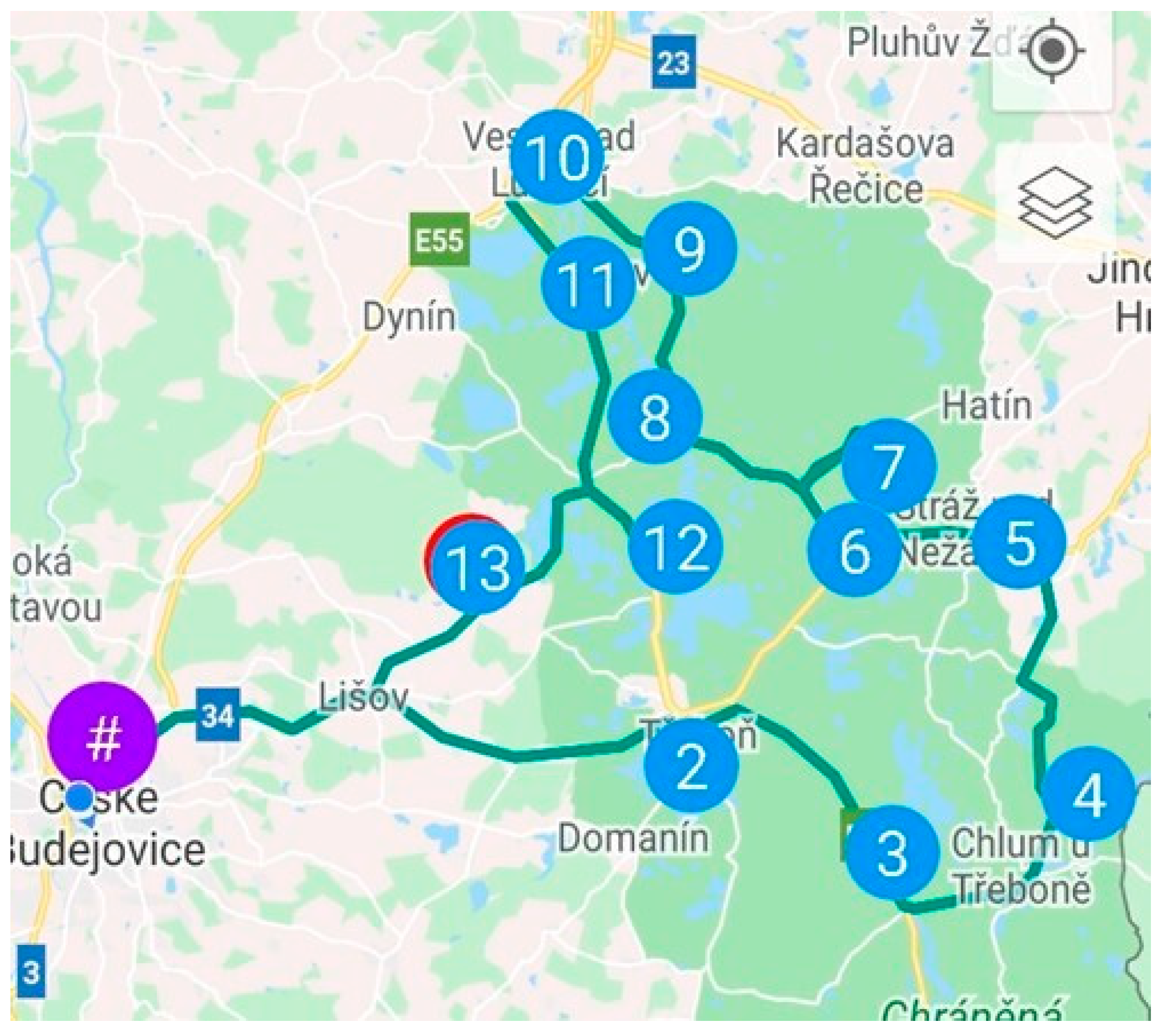Essentially, this application works on the principle of the Greedy algorithm, which is described, for instance, in [39]. For route A, the application proposed the order of the points which is shown in the following Figure 4.

It is now necessary to compare the route thus obtained with the initial route and to determine the order of points as shown in a previous study [39]. From the initial matrix, it is then necessary to find the length and operating time of the selected route [40]. This optimized route leads through the points: A1 ≥ A11 ≥ A10 ≥ A9 ≥ A7 ≥ A8 ≥ A6 ≥ A5 ≥ A4 ≥ A2 ≥ A3 ≥ A12 ≥ A13 ≥ A1.

For route B, the Routin application designed the following order of points: B1 ≥ B2 ≥ B10 ≥ B9 ≥ B7 ≥ B6 ≥ B5 ≥ B4 ≥ B8 ≥ B3 ≥ B1.

For route C, the Routin application designed the following order of points: C1 ≥ C2 ≥ C3 ≥ C4 ≥ C11 ≥ C10 ≥ C9 ≥ C8 ≥ C5 ≥ C6 ≥ C7 ≥ C1.

Final length and the operating time for all individual routes are summarized in the following

Table 21. Optimization with the Routin application—final table for all routes.

Route Name	Operating Time (min)	Length of the Route (km)
Route A	184	154.8
Route B	198	177.9
Route C	187	154.3

.

5. Discussion

In this section, the individual proposed routes are assessed in terms of route length (km) or operating time (min). In the case of both of these indicators, the percentage savings compared to the original route are given. For each route, the operating time is multiplied by the speed difference coefficient, which takes into account real speed measurements in practice [41].

• Technical evaluation of route A

The following

Table 22. Route A—final table of the optimized routes.

Route A	Length of the Route (km)	Percentage Saving Compared to the Length of the Initial Route	Operating Time (min)	Speed Difference Coefficient	Final Operating Time (min)	Percentage Saving Compared to the Operating Time of the Initial Route
Initial route	166.6				212
Hungarian method	158.8	4.68%	181	1.11	201	5.23%
VAM	158.8	4.68%	181	1.11	201	5.23%
Nearest neighbor method	178.2	−6.96%	202	1.11	224	−5.76%
Routin application	154.8	7.08%	184	1.11	204	3.66%

contains a comprehensive summary of optimized routes using the methods of Operations Research, including the original values for the initial route A.

Optimization using the nearest neighbor method proves to be the least advantageous for route A. The Hungarian and VAM methods bring identical results for this route [42]. The Routin application shortens the initial route the most. It therefore depends on the required aspect whether the shortest route or the fastest route is searched. In the case of route A, the shortest route is chosen, as there are greater fuel savings [43]. The following route is selected as the optimal solution, which is created via the Routin application: A1 ≥ A11 ≥ A10 ≥ A9 ≥ A7 ≥ A8 ≥ A6 ≥ A5 ≥ A4 ≥ A2 ≥ A3 ≥ A12 ≥ A13 ≥ A1.

Through this route, the traffic performance of vehicles on route A will be reduced by 7.08% and the time required to operate the route will be reduced by 3.66%.

Technical evaluation of route B

The following

Table 23. Route B—final table of the optimized routes.

Route B	Length of the Route (km)	Percentage Saving Compared to the Length of the Initial Route	Operating Time (min)	Speed Difference Coefficient	Final Operating Time (min)	Percentage Saving Compared to the Operating Time of the Initial Route
Initial route	181.2				221
Hungarian method	178.3	1.60%	199	1.122	223	−1.03%
VAM	178.3	1.60%	199	1.122	223	−1.03%
Nearest neighbor method	177.9	1.82%	198	1.122	222	−0.52%
Routin application	177.9	1.82%	198	1.122	222	−0.52%

shows the length of optimized routes and their final operating time for route B.

To find the optimized route, the nearest neighbor method and the Routin application can be used with final length of 177.9 km and an operating time of 222 min. Both of these routes will reduce traffic performance of vehicles on route B by 1.82%, while the time needed to operate the route will increase by 0.52%.

The nearest neighbor method chooses the following order of service points: B1 ≥ B9 ≥ B10 ≥ B7 ≥ B6 ≥B5 ≥ B4 ≥ B8 ≥ B3 ≥ B2 ≥ B1.

The Routin application chooses the following order of service points: B1 ≥ B2 ≥ B10 ≥ B9 ≥ B7 ≥ B6 ≥ B5 ≥ B4 ≥ B8 ≥ B3 ≥ B1.

• Technical evaluation of route C

The following

Table 24. Route C—final table of the optimized routes.

Route C	Length of the Route (km)	Percentage Saving Compared to the Length of the Initial Route	Operating Time (min)	Speed Difference Coefficient	Final Operating Time (min)	Percentage Saving Compared to the Operating Time of the Initial Route
Initial route	166.2				216
Hungarian method	155.5	6.44%	183	1.125	206	4.69%
VAM	170.1	−2.35%	191	1.125	215	0.52%
Nearest neighbor method	155	6.74%	184	1.125	207	4.17%
Routin application	154.3	7.16%	187	1.125	210	2.60%

shows the length of optimized routes and their final operating time for route C.

The route obtained by optimization through the Routin application is based on the shortest route and passes through the following points: C1 ≥ C2 ≥ C3 ≥ C4 ≥ C11 ≥ C10 ≥ C9 ≥ C8 ≥ C5 ≥ C6 ≥ C7 ≥ C1.

In the following

Table 25. Summary calculation—calculation of savings by used methods.

Route	Total Fuel Costs	Total Fuel Costs for Each Route	Total Fuel Cost Savings for Each Route	Percentage Fuel Cost Savings on Each Route
A	EUR 3280.21	EUR 3047.88	EUR 232.33	7.08%
B	EUR 3548.45	EUR 3483.83	EUR 64.62	1.82%
C	EUR 3314.65	EUR 3077.32	EUR 237.33	7.16%
	Total fuel costs in 2019		Total fuel costs in 2020	Total expected financial savings after optimization
	EUR 10,143.31	EUR 9609.03	EUR 534.28	5.27%

, a summary calculation of savings by using all three methods is presented.

The economic evaluation listed in the above table complements the technical evaluation and focuses on the calculation of operating costs associated with fuel consumption [44]. The total expected financial savings after optimization reached 5.27%.

6. Conclusions

This paper was devoted to the optimization of pick-up and delivery activities and to the technical and economical evaluation of such an optimization. For the application part, i.e., optimization of individual routes, first of all, it was necessary to compile the professional context of the problem, which forms the theoretical part of the work. The application part of the manuscript includes the introduction of the addressed problem as well as the methodological section.

The main part of this study then deals with the very optimization of the pick-up routes and the technical and economic evaluation of this optimization. To this end, in order to address the vehicle routing problem, the Hungarian method, the Vogel approximation method and the nearest neighbor method were determined to be the adequate methods of Operations Research. The Hungarian method is based on a uniform distance matrix and its application is universal. The Vogel approximation method and the nearest neighbor method were used since they use the same input matrix as the Hungarian method and are thus suitable for mutual comparison. To complement these methods, the Routin route planner was applied, which is a publicly available intuitive application that optimizes distribution routes.

For each distribution route separately, input matrices were generated, which contain all the operated unloading points of the given route and their mutual distance value. These matrices are necessary for optimization using the defined techniques being applied to the discussed distribution problem.

This was followed by the technical and economic evaluation of the work results, which assesses the results of the optimization in terms of saving time and transport performance, as well as the economic aspect. As for route A, the newly designed route managed to reduce transport performance by 7.08% and the time required to operate this route also decreased by 3.66%. In regard to route B, transport performance decreased by 1.82%, whereby the time required to operate the route increased by 0.52%. As far as route C is concerned, transport performance decreased by 7.16% and the time required to operate the route was reduced by 2.6%.

Regarding the used methods, it can be stated that the Hungarian method and optimization using the Routin application brought the most efficient results. However, in general, we must state that it is not possible to choose the best possible method of optimization, because each can bring different results in terms of route length and in terms of operation speed, and it depends on which of these variables is preferred for optimization. In our case, the shortest route was sought, and in all the cases, the Routin application found it. Nevertheless, it is appropriate to use a wider range of methods, because then the ability to compare the results obtained increases and thus approaches the optimal solution.

The economic evaluation provided in the Discussion section focuses on the calculation of fuel costs valid in the case that the selected company decides to start these new optimized routes and change its current distribution routes. The economic evaluation compares the fuel costs on the original routes with the newly optimized routes. Assuming the same fuel costs, a saving of EUR 534.28 per year is calculated here, which means a reduction in fuel costs by 5.27% for all the routes together.

As for the further research, the introduction of some specific telematics tools should represent an option in terms of searching for optimal distribution routes. Currently, telematics devices are important both when providing logistics services and when executing transport operations, and their interconnection with the surroundings is inevitable. To maintain an efficient distribution system (i.e., delivery routes), it is imperative to design the concept of telematics interconnection of on-line information related to several transport modes and kinds of logistics services—their optimal deployment, utilization of their capacities with regard to transport infrastructure capacity, fuel prices, tolls, charges for infrastructure with respect to the environment, etc. The basic idea is to create a platform, by corresponding HW and SW, for the telematics flow of processes inside logistics objects and among individual parties involved. To this end, it is important to know the development outlook directions of the transport and logistics market, the participants and requirements of customers in terms of services provided.