Article

Accurate Numerical Treatment on a Stochastic SIR Epidemic Model with Optimal Control Strategy

1
Department of Science in Engineering, Faculty of Engineering, International Islamic University Malaysia, Kuala Lumpur 53100, Malaysia
2
Department of Mechatronics Engineering, Faculty of Engineering, International Islamic University Malaysia, Kuala Lumpur 53100, Malaysia
3
Department of Teaching English as Second Language, Faculty of Education, International Islamic University Malaysia, Kuala Lumpur 53100, Malaysia
4
Faculty of Pharmacy, Universiti Kebangsaan Malaysia, Kuala Lumpur 50300, Malaysia
5
School of Industrial & Systems Engineering, University of Oklahoma, Norman, OK 73019, USA
6
Computer and Information Science, Clark Atlanta University, Atlanta, GA 30314, USA
*
Author to whom correspondence should be addressed.
Technologies 2022, 10(4), 82; https://doi.org/10.3390/technologies10040082
Submission received: 4 April 2022 / Revised: 6 June 2022 / Accepted: 4 July 2022 / Published: 6 July 2022

Abstract

:
In this paper, a numerical study has been undertaken on the susceptible-infected-recovered (SIR) epidemic model that encompasses the mechanisms of the evolution of disease transmission; a prophylactic vaccination strategy in the susceptible populations, depending on the infective individuals. We furnish numerical and graphical simulation combined with explicit series solutions of the proposed model using the New Iterative Method (NIM) and Modified New Iterative Method (MNIM). The analytic-numeric New Iterative Method failed to deliver accurate solution for the large time domain. A new reliable algorithm based on NIM, the coupling of the Laplace transforms, and the New Iterative method is called Modified New Iterative Method (MNIM) which is presented to enhance the validity domain of NIM techniques. The convergence analysis of the MNIM has also been illustrated. The simulation results show that the vaccination strategy can slow down the spread of the epidemic rapidly. Numerical results illustrate the excellent performance of the MNIM and show that the modified method is much more accurate than the NIM.

1. Introduction

The relation between the biology of infectious diseases, the propagation mechanism, and the mathematics used to explain them is a vital research undertaking. Infectious diseases frequently affect a significant number of populations across a wide geographical area. Experiments undertaken in laboratories are insufficient due to the vast differences in scale. Large-scale trials on infectious diseases in humans are not feasible or immoral [1]. Therefore, various mathematical models have been designed and utilized to obtain insight into the dynamics of transmission and control of the epidemic. To combat the risks of contagious epidemic diseases, it is critical to reducing the peak time of epidemic disease to slow down the inevitable dynamics and prepare for the subsequent epidemic wave [2].
In the past decades, the global scientific community has developed several mathematical models for the transmission and prevention of infectious diseases such as childhood disease [3], HIV/AIDS [4], dengue [5], tuberculosis [6], Ebola [7], COVID-19 [8,9,10,11,12,13] and many others. These models are very critical in diverse areas, such as policy making, emergency planning, risk management, prevention strategies, and the implementation of the enhancement of various health and economic aspects [14]. However, there is still a lack of numerical studies that can help the researcher to understand the disease transmission rate, infection rate, and recovery rate in the epidemic situation.
The susceptible-infected-recovered (SIR) model of epidemiological type, first proposed by Kermack and Mckendrick [15], is an epidemic model for the spread of infectious disease. In order to conduct the numerical study of the dynamics of such diseases, we considered the susceptible-infected-recovered (SIR) epidemiologic nonlinear mathematical model which is being created by O.D. Makinde [3] to track the temporal dynamics of a pediatric illness in the presence of a preventative vaccination strategy. In particular, compartmental relations are used to describe an infection state and a process of infection by dividing the population into compartments based on assumptions about the nature and rate of transfer from one compartment to another. The rate of leaving the compartment depends only on the current state of the epidemic [16].
Figure 1 demonstrates the SIR model of childhood infectious disease [17] contains a susceptible group, symbolized by S , an infected group I , and a recovered group R , which denotes a vaccinated, as well as recovered people with constant immunity. It assumes that the vaccine efficacy is 100% and the fraction of citizens vaccinated at birth, each year are denoted as p (with 0 < p < 1 ) and the remain populations ( 1 p ) are susceptible. A susceptible individual move into the infected group through communication with an infected individual by an average contact rate b . A person who has been infected, recovers at a rate of c and enters recovered group. The recovered group also contain vaccinated individual. The differential equations for the SIR model follow the natural death rates μ and the birth rates a . Therefore, the size of population N is not stable.
The rates of change of the three populations are determined by the following system of three coupled nonlinear ordinary differential equations [17] used in this analysis
S = ( 1 p ) a N μ S ( t ) b S ( t ) I ( t ) N ,
I = b S ( t ) I ( t ) N ( c + μ ) I ( t ) ,
R = p a N + c I ( t ) μ R ( t )
Here, all parameters p ,   a ,   b ,   c ,   μ are positive constants. The total population N varies with respect to time t (in year) as we assume that a μ . To make sure that the overall population N is always inconsistent, we add the equations contain in the system (1)–(3) to obtain
d N d t = ( a μ ) N ,
Each group’s size is proportional to the total population, rearranging the above system (1)–(3) by assuming S N = x ,   I N = y ,   R N = z ; we obtained the following expression:
x = ( 1 p ) a a x ( t ) b y ( t ) x ( t ) ,
y = b y ( t ) x ( t ) ( c + a ) y ( t ) ,
z = p a + c y ( t ) a z ( t )
Therefore, this study 3 focused on solving the system (5)–(7) with initial conditions (Ics)—
x ( 0 ) = s 0 , y ( 0 ) = i 0 , z ( 0 ) = r 0
In our literature survey, we found that the approximate analytical solutions of the childhood SIR infectious disease model were presented first time by Makinde [3], using the Adomian decomposition method (ADM). Yildirim and Cherruault [18] derived the approximate analytical expression for the SIR model using the Homotopy perturbation method (HPM). Recently, Mungkasi [17] corrected the inaccurate solutions of Ghotbi et al. [19] by using successive approximation methods to the determined system. Srivastava and Günerhan [20] introduced the conformable fractional differential transform method (CFDTM) to calculate an approximate solution of the fractional-order susceptible-infected-recovered (SIR) epidemic model of childhood disease. The combined technique of the classical homotopy perturbation method and the Elzaki transform have been utilized by Jena et.al [21] to solve the childhood diseases model with fractional order.
In this research, we have revisited the model in order to provide a numerical framework via New Iterative Method (NIM) and Modified New Iterative Method (MNIM). The current study investigates the well-documented SIR infection model to test the validity domain of the proposed methods with straightforward computations. For this particular form of SIR model, the analytical solutions have been derived using a coalescence of Laplace transform and the New Iterative Method, which is called modified NIM. We also use the NIM scheme which is based on the iterative principle of characteristics, introduced by Daftardar-Gejji and Jafari [22]. Recently, the application of NIM can be found in the literature specifically dealing with Klein-Gordon equations [23], fractional Whitham-Broer-Kaup (WBK) system [24], Fisher’s equation [25], Cahn-Hillard equation [26], multidimensional wave equations [27], 1D Swift–Hohenberg equation [28], Falkner-Skan Equation [29], Jeffery-Hamel flow problem [30], Chemical kinetics equations [31,32], Lake pollution model [33] and many other problems. Stability analysis, Error bound, and Convergence analysis of NIM have been illustrated in Refs. [33,34].

2. Solution Procedure

2.1. New Iterative Method

In this section, a class of n-th-order differential equation has been considered in the form,
u ( n ) ( t ) = f ( t , u ( t ) , u ( t ) , u ( t ) , u ( n 1 ) ( t ) ) , 0 t T ,
Subject to the initial conditions
u ( t 0 ) = u 0 , u ( t 0 ) = u 0 , u ( t 0 ) = u 0 , u ( n 1 ) ( t 0 ) = u 0 n 1 ,
where f is a time dependent, continuous linear/nonlinear function and u 0 , u 0 , u 0 , u 0 n 1 are prescribed. Now the operator form of the above equation can be written as,
L u = R ( u ) + N ( u ) + g ( t ) ,
where f ( t , u ( t ) , u ( t ) , u ( t ) , u ( n 1 ) ( t ) ) = R u + N u + g ( t ) , and L d n d t n is chosen to be highest order derivative, which is easily invertible, R u the remaining linear differential operator whose order is less than L ;  N u represents the nonlinear terms and g is the given inhomogeneous source term. The Equation (11) can now be rewritten as:
L u = g + R u + N u ,
Applying the inverse operator L 1 to both sides of (12),
u = f ( t ) + L 1 R u + L 1 N u ,
where f ( t ) is the term arising from integrating the source term g ( t ) .
Let, the solution of Equation (13) for u may be written in the series:
u ( t ) = i = 0 u i = u 0 + u 1 + u 2 +
The nonlinear term N   can be find out as
H 0 = N ( u 0 )   and   H m = N ( j = 0 m u j ) N ( j = 0 m 1 u j ) .
Thus, according to NIM,
N ( i = 0 u i ) = H 0 + H 1 + H 2 +   = N ( u 0 ) + ( N ( u 0 + u 1 ) N ( u 0 ) ) + ( N ( u 0 + u 1 + u 2 ) N ( u 0 + u 1 ) ) +
Now, we define the recurrence relation as follows:
u 0 = L 1 g ( t ) + φ = f ( t ) ,
u 1 = L 1 R ( u 0 ) + L 1 ( H 0 ) ,
u m + 1 = L 1 R ( u m ) + L 1 ( H m ) ,   m 1
Since R is linear then,
( i = 0 m R u i ) = R ( i = 0 u i )
Then series solution becomes
i = 1 u i = f ( t ) + L 1 R ( i = 0 u i ) + L 1 N ( i = 0 u i )
Now, the n-term solution can be written as series form as:
u = i = 0 n 1 u i = u 0 + u 1 + u 2 + + u n 1 .

2.2. Modified New Iterative Method

We have proposed an improvement of NIM based on the composition of Laplace transform with the New Iterative Method to solve system of differential equations.
Let us consider a system of differential equations in the operator form:
D ( μ 1 ) + R 1 ( μ 1 ) + N 1 ( μ 1 , μ 2 , ... , μ n ) = g 1 ( t ) ,
D ( μ 2 ) + R 2 ( μ 2 ) + N 2 ( μ 1 , μ 2 , ... , μ n ) = g 2 ( t ) ,
D ( μ n ) + R n ( μ n ) + N n ( μ 1 , μ 2 , ... , μ n ) = g n ( t ) ,
Subjected to the initial conditions.
μ 1 ( 0 ) = a 1 , μ 2 ( 0 ) = a 2 , ... , μ n ( 0 ) = a n ,
where D is a invertible linear differential operator, and R 1 , R 2 , ... , R n are remaining linear operators order less than D and N 1 , N 2 , ... , N n are nonlinear operators and g 1 , g 2 , ... , g n are inhomogeneous terms. For the first order D d d t , second order D d 2 d t 2 and so on.
The technique consists first of applying Laplace transformation (which is denoted by ) to both sides of systems (23)–(25), hence
{ D ( μ 1 ) } + { R 1 ( μ 1 ) } + { N 1 ( μ 1 , μ 2 , ... , μ n ) } = { g 1 ( t ) } ,
{ D ( μ 2 ) } + { R 2 ( μ 2 ) } + { N 2 ( μ 1 , μ 2 , ... , μ n ) } = { g 2 ( t ) } ,
{ D ( μ n ) } + { R n ( μ n ) } + { N n ( μ 1 , μ 2 , ... , μ n ) } = { g n ( t ) }
Applying the formulas for Laplace transforms, we obtain
s ( μ 1 ) μ 1 ( 0 ) = { g 1 ( t ) } { R 1 ( μ 1 ) } { N 1 ( μ 1 , μ 2 , ... , μ n ) } ,
s ( μ 2 ) μ 2 ( 0 ) = { g 2 ( t ) } { R 2 ( μ 2 ) } { N 2 ( μ 1 , μ 2 , ... , μ n ) } ,
s ( μ n ) μ n ( 0 ) = { g n ( t ) } { R n ( μ n ) } { N n ( μ 1 , μ 2 , ... , μ n ) } ,
where ‘ s ’ is called a Laplace domain function.
Using the initial conditions (26), we have,
( μ 1 ) = a 1 s + { g 1 ( t ) } s 1 s { R 1 ( μ 1 ) } 1 s { N 1 ( μ 1 , μ 2 , ... , μ n ) } ,
( μ 2 ) = a 2 s + { g 2 ( t ) } s 1 s { R 2 ( μ 2 ) } 1 s { N 2 ( μ 1 , μ 2 , ... , μ n ) } ,
( μ n ) = a n s + { g n ( t ) } s 1 s { R n ( μ n ) } 1 s { N n ( μ 1 , μ 2 , ... , μ n ) } ,
Applying the inverse Laplace transform to the equations in (33)–(35), we get
μ 1 = 1 [ a 1 s + { g 1 ( t ) } s ] 1 s 1 [ { R 1 ( μ 1 ) } ] 1 s 1 [ { N 1 ( μ 1 , μ 2 , ... , μ n ) } ] ,
μ 2 = 1 [ a 2 s + { g 2 ( t ) } s ] 1 s 1 [ { R 2 ( μ 2 ) } ] 1 s 1 [ { N 2 ( μ 1 , μ 2 , ... , μ n ) } ] ,
μ n = 1 [ a 2 s + { g n ( t ) } s ] 1 s 1 [ { R n ( μ n ) } ] 1 s 1 [ { N n ( μ 1 , μ 2 , ... , μ n ) } ]
Let, the approximate the solutions μ 1 , μ 2 , ... , μ n of system (36)–(38) can be expressed as
μ 1 = μ 1 , 0 + μ 1 , 1 + = i = 0 μ 1 , i ,
μ 2 = μ 2 , 0 + μ 2 , 1 + = i = 0 μ 2 , i ,
μ n = μ n , 0 + μ n , 1 + = i = 0 μ n , i .
For the NIM, the nonlinear operators can be decomposed by,
G 0 = N 1 ( μ 1 , 0 )   and   G m = N 1 ( i = 0 m μ 1 , i ) N 1 ( i = 0 m 1 μ 1 , i ) , m 1 ,
H 0 = N 2 ( μ 2 , 0 )   and   H m = N 2 ( i = 0 m μ 2 , i ) N 2 ( i = 0 m 1 μ 2 , i ) , m 1 ,
I 0 = N n ( μ n , 0 )   and   I m = N n ( i = 0 m μ n , i ) N n ( i = 0 m 1 μ n , i ) , m 1
Thus, the nonlinear operators can be expressed as:
N 1 ( i = 0 μ 1 , i ) = N 1 ( μ 1 , 0 ) + { N 1 ( μ 1 , 0 + μ 1 , 1 ) N 1 ( μ 1 , 0 ) } + { N 1 ( μ 1 , 0 + μ 1 , 1 + μ 1 , 2 ) N 1 ( μ 1 , 0 + μ 1 , 1 ) } + ,
N 2 ( i = 0 μ 2 , i ) = N 2 ( μ 2 , 0 ) + { N 2 ( μ 2 , 0 + μ 2 , 1 ) N 2 ( μ 2 , 0 ) } + { N 2 ( μ 2 , 0 + μ 2 , 1 + μ 2 , 2 ) N 2 ( μ 2 , 0 + μ 2 , 1 ) } + ,
N n ( i = 0 μ n , i ) = N n ( μ n , 0 ) + { N n ( μ n , 0 + μ n , 1 ) N n ( μ n , 0 ) } + { N n ( μ n , 0 + μ n , 1 + μ n , 2 ) N n ( μ n , 0 + μ n , 1 ) } +
Since R 1 , R 2 , ... , R n are linear.
i = 0 R 1 ( μ 1 , i ) = R 1 ( i = 0 μ 1 , i ) ,
i = 0 R 2 ( μ 2 , i ) = R 2 ( i = 0 μ 2 , i ) ,
i = 0 R n ( μ n , i ) = R n ( i = 0 μ n , i )
The NIM admits the use of the recursive relations by following way:
μ 1 , 0 = 1 [ { g 1 ( t ) } s ] + a 1 = f 1 ( t ) + a 1 ,
where f 1 ( t ) is the term arising after inverse Laplace transformation of the source term { g 1 ( t ) } s , all of which are assumed to be prescribed.
μ 1 , 1 = 1 [ 1 s { R 1 ( μ 1 , 0 ) } ] 1 s 1 [ ( G 0 ) ] ,
μ 1 , m + 1 = 1 [ 1 s { R 1 ( μ 1 , m ) } ] 1 [ 1 s ( G m ) ] , m = 1 , 2 , ... .
Thus,
μ 1 = i = 0 μ 1 , i = f 1 + i = 1 μ 1 , i = f 1 1 [ 1 s { R 1 ( i = 0 μ 1 , i ) } ] 1 [ 1 s { N 1 ( i = 0 μ 1 , i ) } ]
By the similar manner, we have
μ 2 , 0 = 1 [ { g 2 ( t ) } s ] + a 2 = f 2 ( t ) + a 2 ,
μ 2 , 1 = 1 [ 1 s { R 2 ( μ 2 , 0 ) } ] 1 [ 1 s ( H 0 ) ] ,
μ 2 , m + 1 = 1 [ 1 s { R 2 ( μ 2 , m ) } ] 1 [ 1 s ( H m ) ] , m = 1 , 2 , ... ,
μ 2 = i = 0 μ 2 , i = f 2 + i = 1 μ 2 , i = f 2 1 [ 1 s { R 2 ( i = 0 μ 2 , i ) } ] 1 [ 1 s { N 2 ( i = 0 μ 2 , i ) } ] ,
and
μ n , 0 = 1 [ { g n ( t ) } s ] + a n = f n ( t ) + a n ,
μ n , 1 = 1 [ 1 s { R n ( μ n , 0 ) } ] 1 [ 1 s { I 0 } ] ,
μ n , m + 1 = 1 [ 1 s { R n ( μ n , m ) } ] 1 [ 1 s { I m } ] , m = 1 , 2 , ... ,
μ n = i = 0 μ n , i = f n + i = 1 μ n , i = f n 1 [ 1 s { R n ( i = 0 μ n , i ) } ] 1 [ 1 s { N n ( i = 0 μ n , i ) } ]
The k -terms approximate solutions are given by the following form:
μ 1 = i = 0 k 1 μ 1 , i = μ 1 , 0 + μ 1 , 1 + μ 1 , 2 + + μ 1 , k 1 ,
μ 2 = i = 0 k 1 μ 2 , i = μ 2 , 0 + μ 2 , 1 + μ 2 , 2 + + μ 2 , k 1 ,
μ n = i = 0 k 1 μ n , i = μ n , 0 + μ n , 1 + μ n , 2 + + μ n , k 1 .

2.3. Convergence Analysis of MNIM

Let, Χ , ϒ and κ be the elements in a Banach space B and N is nonlinear contraction from B B such that κ = N ( Χ ) N ( ϒ ) σ Χ ϒ ,   0 < σ < 1 . Then we can prove that κ r + 1 σ r + 1 κ 0 , r = 0 , 1 , ... by the principle of Banach fixed point theorem.
Let, κ 0 is the initial approximation and ρ is a known function in Banach Space B .
κ 0 ( t ) = ρ ( t ) ,
By the decomposition principle of nonlinear terms in MNIM, we can write
κ 1 = N ( κ 0 ) σ κ 0 ,
κ 2 = N ( κ 0 + κ 1 ) N ( κ 0 ) σ κ 1 σ 2 κ 0 ,
κ 3 = N ( κ 0 + κ 1 + κ 2 ) N ( κ 0 + κ 1 ) σ κ 2 σ 2 κ 1 σ 3 κ 0 ,
κ r + 1 = N ( j = 0 r κ j ) N ( j = 0 r 1 κ j ) σ κ r σ r + 1 κ 0 , r = 0 , 1 , 2 , ... .
Hence, the solutions of MNIM procedure converges via Banach fixed point theorem.

3. Application

3.1. Solutions by NIM

To check the validity of NIM solutions we have solved the problem by NIM method. Let us take the integration on the system (5)–(7), we obtain:
x ( t ) = s 0 + ( 1 p ) a t ( 0 t a x ( t ) d t ) ( 0 t b y ( t ) x ( t ) d t ) ,
y ( t ) = i 0 + ( 0 t b y ( t ) x ( t ) d t ) ( 0 t ( c + a ) y ( t ) d t ) ,
z ( t ) = r 0 + p a t + ( 0 t c y ( t ) d t ) ( 0 t a z ( t ) d t )
In view of Equations (17)–(19) and according to the solution procedure of NIM for system of differential equations, we find the approximations as follows:
x 0 ( t ) = s 0 + ( 1 p ) a t ,
y 0 ( t ) = i 0 ,
z 0 ( t ) = p a t + r 0 ,
x 1 ( t ) = ( 1 p ) a 2 t 2 2 a s 0 t b i 0 ( 1 p ) a t 2 2 b i 0 s 0 t ,
y 1 ( t ) = b i 0 ( 1 p ) a t 2 2 + b i 0 s 0 t ( c + a ) i 0 t ,
z 1 ( t ) = c i 0 t 1 2 p a 2 t 2 a r 0 t ,
Similarly, we can obtain the other approximations as well. Therefore, the approximate precisions are:
x ( t ) = i = 0 x i ( t ) ,
y ( t ) = i = 0 y i ( t ) ,
z ( t ) = i = 0 z i ( t ) .

3.2. Solutions by MNIM

By applying Laplace Transform on the system of Equations (5)–(7), and using ICs (8), we obtain:
( x ( t ) , t , ε ) = 1 ε + a ( a ( p 1 ) ε + s 0 b ( y ( t )   x ( t ) , t , ε ) ) ,
( y ( t ) , t , ε ) = 1 ε + a + c ( i 0 + b ( y ( t ) x ( t ) , t , ε ) ) ,
( z ( t ) , t , ε ) = 1 ε + a ( p a ε + r 0 + c ( y ( t )   , t , ε ) ) ,
Taking inverse Laplace transform operator on (83)–(85), we get:
x ( t ) = 1 { 1 ε + a ( a ( p 1 ) ε + s 0 b ( y ( t ) x ( t ) , t , ε ) ) } ,
y ( t ) = 1 { 1 ε + a + c ( i 0 + b ( y ( t ) x ( t ) , t , ε ) ) } ,
z ( t ) = 1 { 1 ε + a ( p a ε + r 0 + c ( y ( t )   , t , ε ) ) } ,
In view of (51)–(62), we can obtain the following iterations by using MNIM,
x 0 ( t ) = 1 { 1 ε + a ( a ( p 1 ) ε + s 0 ) } = 1 p + ( p + s 0 1 ) e a t ,
y 0 ( t ) = 1 { i 0 ε + a + c } = i 0 e ( c + a ) t ,
z 0 ( t ) = 1 { p a ε + r 0 ε + a } = p + ( p + r 0 ) e a t ,
x 1 ( t ) = ( e ( c + 2 a ) t c ( p + s 0 1 ) ( p 1 ) e ( c + a ) t ( c + a ) + e a t ( p a c s 0 a ) ) i 0 b c ( c + a ) ,
y 1 ( t ) = ( e ( c + 2 a ) t ( p s 0 + 1 ) + ( a p t + a t + p + s 0 1 ) e ( c + a ) t ) i 0 b a ,
z 1 ( t ) = i 0 ( e ( c + a ) t + e a t ) ,
and so on. In the similar approach the further components can be obtained. Therefore, the approximate precisions are
x ( t ) = i = 0 x i ( t ) ,
y ( t ) = i = 0 y i ( t ) ,
z ( t ) = i = 0 z i ( t ) .

4. Results and Discussions

We take the initial conditions s 0 = 0.8 , i 0 = 0.2 , r 0 = 0 and parameters values p = 0.9 , a = 0.4 , b = 0.8 ,   c = 0.03 ; a similar scenario of ref. [3]. All our calculations as well as our graphs are carried out by Maple 2020. We set the continuous constant step size h = 0.001 for the RK4 in the maple software.

4.1. NIM Solutions

Therefore, 5-iterations of NIM solutions are:
x ( t ) = i = 0 5 x i ( t ) = 6.736115226612228 × 10 52 t 47 + 3.922133162637945 × 10 49 t 46 + 1.073655848446378 × 10 46 t 45 + 1.844655274257630 × 10 44 t 44 + 2.242032611955568 × 10 42 t 43 + 2.060673733084379 × 10 40 t 42 + 1.494716735333350 × 10 38 t 41 + 8.809612654525537 × 10 37 t 40 + 4.305357070507673 × 10 35 t 39 + 1.768963027457917 × 10 33 t 38 + 6.164360273888642 × 10 32 t 37 + 1.829859631340267 × 10 30 t 36 + 4.627443481597180 × 10 29 t 35 + 9.920911834830423 × 10 28 t 34 + 1.782386359157935 × 10 26 t 33 + 2.622401070812103 × 10 25 t 32 + 3.013741998638641 × 10 24 t 31 + 2.397281814414504 × 10 23 t 30 + 7.028239936204403 × 10 23 t 29 1.230670827410604 × 10 21 t 28 2.070457639465569 × 10 20 t 27 1.239142909703323 × 10 19 t 26 + 2.949835075276537 × 10 19 t 25 + 3.725341255626546 × 10 17 t 23 3.435588549817450 × 10 16 t 22 + 9.557233694959134 × 10 18 t 24 2.904383929261819 × 10 15 t 21 + 1.169109476870975 × 10 14 t 20 + 1.575620033256645 × 10 13 t 19 4.676372541642090 × 10 13 t 18 6.907013200303840 × 10 12 t 17 + 2.695714904867200 × 10 11 t 16 + 1.988585322443935 × 10 10 t 15 1.490922789811607 × 10 9 t 14 6.672613505299390 × 10 10 t 13 + 3.610221503703013 × 10 8 t 12 5.718040776900796 × 10 8 t 11 7.848058588316446 × 10 7 t 10 + 4.260175583211709 × 10 6 t 9 1.110385716627811 × 10 6 t 8 0.00005754643154102856 t 7 + 0.0001517085007466667 t 6 + 0.0002838500160000001 t 5 0.001811776 t 4 0.008224 t 3 + 0.1008 t 2 0.408 t + 0.8 ,
y ( t ) = i = 0 5 y i ( t ) = 6.736115226612228 × 10 52 t 47 3.922133162637945 × 10 49 t 46 1.073655848446378 × 10 46 t 45 1.844655274257630 × 10 44 t 44 2.242032611955568 × 10 42 t 43 2.060673733084379 × 10 40 t 42 1.494716735333350 × 10 38 t 41 8.809612654525537 × 10 37 t 40 4.305357070507673 × 10 35 t 39 1.768963027457917 × 10 33 t 38 6.164360273888642 × 10 32 t 37 1.829859631340267 × 10 30 t 36 4.627443481597180 × 10 29 t 35 9.920911834830423 × 10 28 t 34 1.782386359157935 × 10 26 t 33 2.622401070812103 × 10 25 t 32 3.013741998638641 × 10 24 t 31 2.397281814414504 × 10 23 t 30 7.028239936204403 × 10 23 t 29 + 1.230670827410604 × 10 21 t 28 + 2.070457639465569 × 10 20 t 27 + 1.239142909703323 × 10 19 t 26 2.949835075276537 × 10 19 t 25 9.557233694710467 × 10 18 t 24 3.725341248233134 × 10 17 t 23 + 3.435588646687410 × 10 16 t 22 + 2.904384680530290 × 10 15 t 21 1.169105545529128 × 10 14 t 20 1.575605121898856 × 10 13 t 19 + 4.676793838257692 × 10 13 t 18 + 6.907896025018594 × 10 12 t 17 2.694385690830112 × 10 11 t 16 1.987319350530539 × 10 10 t 15 + 1.491344335393742 × 10 9 t 14 + 6.609946732092200 × 10 10 t 13 3.617958560529853 × 10 8 t 12 + 5.712957034873109 × 10 8 t 11 + 7.885699621920298 × 10 7 t 10 4.260056651414198 × 10 6 t 9 + 9.012201347078117 × 10 7 t 8 + 0.00005827143817874285 t 7 0.0001487855181688889 t 6 0.0003762609485 t 5 + 0.002759918749999999 t 4 0.0011697 t 3 0.02823 t 2 + 0.042 t + 0.2 ;
z ( t ) = i = 0 5 z i ( t ) = 2.486673133813368 × 10 28 t 24 7.393412085355813 × 10 26 t 23 9.686995915539818 × 10 24 t 22 7.512684713956981 × 10 22 t 21 3.931341846821115 × 10 20 t 20 1.491135778969304 × 10 18 t 19 4.212966156027532 × 10 17 t 18 8.828247147539671 × 10 16 t 17 1.329214037088414 × 10 14 t 16 1.265971913395598 × 10 13 t 15 4.215455821345592 × 10 13 t 14 + 6.266677320718978 × 10 12 t 13 + 7.737056826840045 × 10 11 t 12 + 5.083742027686752 × 10 11 t 11 3.764103360385219 × 10 9 t 10 1.18931797511109 × 10 10 t 9 + 2.091655819199999 × 10 7 t 8 7.250066377142856 × 10 7 t 7 8.611871466666666 × 10 6 t 6 + 0.00009241093249999999 t 5 0.00094814275 t 4 + 0.0093937 t 3 0.07257 t 2 + 0.366 t

4.2. MNIM Solutions

The 3-iterations MNIM solutions are:
6 x ( t ) = i = 0 3 x i ( t ) = 0.1 0.0006017646192844911 e 3.32 t + 0.03925876631627679 e 1.63 t + 0.0007765131412058982 e 2.89 t 0.0002581915613754199 e 2.46 t 8.154807242157790 e 0.4 t + 1.535711286278180 × 10 23 e 1.66 t × ( 3.233242835823126 × 10 17 t 2 + 3.406539138328771 × 10 20 t 4.593848682004663 × 10 21 ) 5.031003559435018 × 10 22 e 0.83   t × ( 5.439324414583916 × 10 18 t 2 + 3.505486748642923 × 10 20 t + 5.176936742877226 × 10 21 ) + 4.232804232804233 × 10 20 e 2.92 t × ( 2.774146215816360 × 10 15 t 1.179728723726773 × 10 16 ) 8.597701458250771 × 10 25 e 2.52 t × ( 6.834618772122878 × 10 18 t 2 6.887323759231177 × 10 20 t 2.054789750054483 × 10 22 ) 9.360006622204685 × 10 26 e 1.26 t × ( 1.775957335388708 × 10 19 t 3 + 7.601863095513286 × 10 20 t 2 4.338292456048305 × 10 23 t 1.563308625518170 × 10 25 ) 2.012401423774007 × 10 22 e 2.12 t × ( 2.800264785138102 × 10 17 t 2 + 8.054649373251765 × 10 18 t 3.731099912706602 × 10 19 ) 3.205609817180065 × 10 22 e 1.72 t × ( 4.454474776080082 × 10 17 t 2 + 2.940605751880004 × 10 19 t + 4.855607088780105 × 10 20 ) + 7.623376607907109 × 10 23 e 0.86 t × ( 6.229503999994038 × 10 17 t 3 + 8.089326933329536 × 10 19 t 2 + 3.188740492482025 × 10 21 t + 3.781029478577795 × 10 22 ) + 1.481481481481481 × 10 19 e 0.43 t × ( 1.151999999999448 × 10 16 t 2 + 1.459199999999788 × 10 18 t + 5.799796492739982 × 10 19 ) 1.831459902474760 × 10 22 e 2.49 t × ( 9.925997520612579 × 10 17 t + 2.746991500144911 × 10 19 ) 8.287048441320135 × 10 26 e 2.09 t × ( 3.874906263024820 × 10 19 t 2 2.895379542793813 × 10 21 t 4.195395911283663 × 10 23 ) + 1.444445466389612 × 10 27 e 1.69 t × ( 1.065222144015543 × 10 21 t 3 + 2.599021250303810 × 10 22 t 2 5.333298360890297 × 10 23 t + 7.995758255225330 × 10 25 ) + 4.250193528577767 × 10 27 e 1.29 t × ( 2.008732537975042 × 10 21 t 3 + 4.866530225436270 × 10 22 t 2 8.085119609709582 × 10 24 t 2.498760580734028 × 10 26 ) 1.161271592393671 × 10 20 e 1.23 t × ( 5.725610654715977 × 10 17 t + 3.019834074926216 × 10 19 ) + 9.290172739149369 × 10 22 e 2.06 t × ( 7.745644989776837 × 10 16 t 5.254962364229557 × 10 19 ) ,
y ( t ) = i = 0 3 y i ( t ) = 0.0006080113108341571 e 3.32 t + 0.0002620072002134803 e 2.46 t 0.0007859828136596286 e 2.89 t 0.04024023547418371 e 1.63 t + 0.2 e 0.43   t + 2.146561518692274 × 10 23 e 1.72 t × ( 6.806879223943861 × 10 18 t 2 + 4.495935696722963 × 10 20 t + 7.427951840196584 × 10 21 ) 1.248000882960625 × 10 23 e 0.86 t × ( 4.070758399996104 × 10 18 t 3 + 5.304608426664167 × 10 20 t 2 + 2.100624173108962 × 10 22 t + 2.506300632140585 × 10 23 ) + 5.453252023119212 × 10 73 e 0.43 t ( 3.129631015457178 × 10 67 t 3 + 2.816667913913444 × 10 69 t 2 + 7.626816999579977 × 10 70 t + 5.099515294485344 × 10 71 ) + 3.770383636535017 × 10 22 e 2.49 t × ( 4.891759543651175 × 10 17 t + 1.354121357567373 × 10 19 ) + 3.497806001185756 × 10 25 e 2.09 t × ( 9.346391669051500 × 10 18 t 2 6.981744507856679 × 10 20 t 1.012015721679164 × 10 23 ) 1.269602584555373 × 10 26 e 1.69 t ( 1.240774054577326 × 10 20 t 3 + 3.034218295207262 × 10 21 t 2 6.199976787711437 × 10 22 t + 9.312434748632805 × 10 24 ) 3.900002759251952 × 10 26 e 1.29 t × ( 2.265465543829327 × 10 20 t 3 + 5.515152550771495 × 10 21 t 2 9.113544300624442 × 10 23 t 2.821640082696647 × 10 25 ) + 2.5 × 10 19 e 1.23 t × ( 2.759330436007700 × 10 16 t + 1.456588408293963 × 10 18 ) 4.817644623433325 × 10 22 e 2.06 t × ( 1.521132690763403 × 10 17 t 1.031981767729906 × 10 20 ) 4.127108492976661 × 10 24 e 1.66 t × ( 1.232444718144824 × 10 18 t 2 + 1.298549367102396 × 10 21 t 1.748561849689992 × 10 22 ) + 5 × 10 19 e 0.83 t ( 5.883531005499098 × 10 15 t 2 + 3.812288952012609 × 10 17 t + 5.670981666287240 × 10 18 ) 1.548362123191561 × 10 21 e 2.92 t ( 7.675137863758596 × 10 16 t 3.260246630067594 × 10 17 ) + 5.608298265951419 × 10 26 × e 2.52 t ( 1.062808766767887 × 10 20 t 2 1.070860668252633 × 10 22 t 3.195993137216618 × 10 23 ) + 1.348551711300533 × 10 26 × e 1.26 t ( 1.277207436992847 × 10 20 t 3 + 5.483102259736971 × 10 21 t 2 3.119452387482340 × 10 24 t 1.125583065075483 × 10 26 ) + 1.325927750611222 × 10 23 e 2.12 t ( 4.325492835496448 × 10 18 t 2 + 1.245072612909103 × 10 20 t 5.749959513369393 × 10 20 ) ,
z ( t ) = i = 0 3 z i ( t ) = 0.9 + 2.098254299024467 e 0.4 t + 0.4 e 0.415 t sin h ( 0.015 t ) + 0.01953488372093023 e 0.83 t 0.002666666666666667 e 0.43 t × ( 305 + 6 t ) + 0.0009492855151178018 e 1.23 t 0.001129388038067028 e 1.66 t 5.897086477312794 × 10 51 e 0.83 t × ( 3.551083966805075 × 10 46 t + 5.211845325099965 × 10 48 ) + 3.944516546299514 × 10 50 e 1.26 t ( 3.552306787033270 × 10 45 t 1.231131263500689 × 10 46 ) + 1.651476380411790 × 10 48 e 0.86 t × ( 2.162937792347110 × 10 46 + 6.269476779331703 × 10 44 t ) 1.552529119388551 × 10 61 e 0.43 t ( 4.122305932992456 × 10 57 t 2 + 4.191011031876038 × 10 59 t + 1.422695266527552 × 10 61 )

4.3. Comparison of the Solutions for SIR Epidemic Model

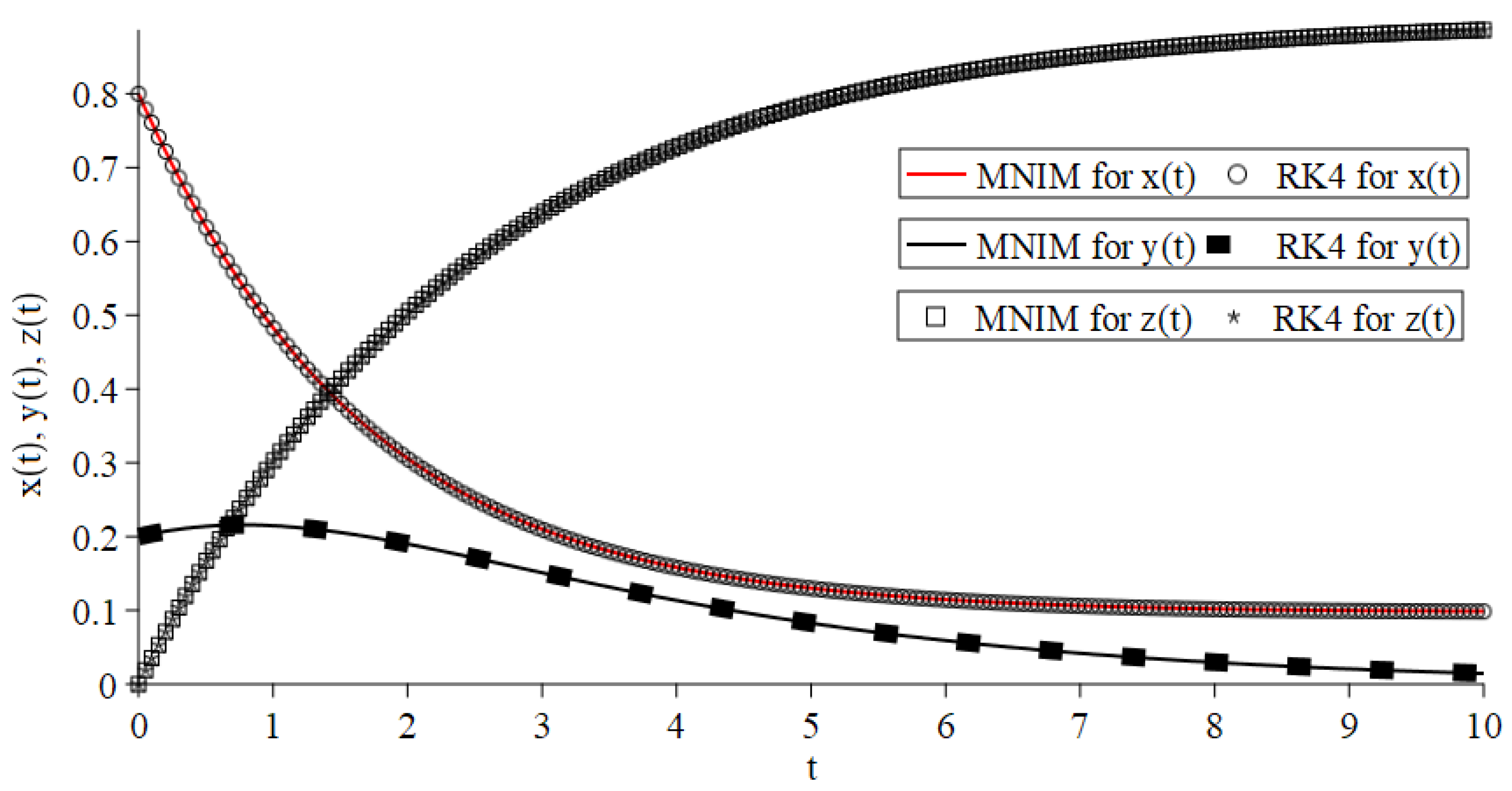
The transmission dynamics of the SIR disease model has been studied numerically. We have coded the New Iterative Method (NIM) and Modified New Iterative Method (MNIM) algorithms for SIR model to test the validity of proposed methods. We have done comparison of absolute errors between ADM [3], NIM and MNIM with respect to RK4 method in Table 1. The MNIM solutions match with RK4 at least 4 decimal places, while both the ADM and NIM solutions are diverging in nature as the value of time t increases. In Figure 2, it can be clear that the 5-iterations of NIM solutions are getting inaccurate as time t gets longer, in contrast the 3-iterations of modified NIM provide excellent accuracy compared to RK4. We have also displayed comparison between RK4 and MNIM on the time interval [ 0 , 10 ] in Figure 3. The comparisons clearly emphasized the accuracy and validity of the MNIM and RK4, as both outcomes clearly overlap each other over a ten-year time period.
Figure 2a shows that the proportion of susceptible individuals decreases exponentially in the total population. In addition, Figure 2b indicates that the infected population increases suddenly when the epidemic is at its pick level, and after a certain period of time it slow down. Consequently, Figure 2c illustrates that the number of recovered individuals increases rapidly within five years of the epidemic. The impact of high vaccination coverage on the initial population groups with low levels of infection rates, as depicted in Figure 3. The populations of the susceptible and infectious groups decline over time, meanwhile the population of the recovered group grows due to the inclusion of vaccinated and recovered people with permanent immunity, and the disease outbreak stops.
In addition, traditional numerical approaches, such as the Runge–Kutta method, can produce approximate-numeric results. However, analytical series solutions to differential equations can be required. Numerical methods, by nature, cannot yield explicit series solutions. Moreover, the Runge–Kutta method cannot provide the discretized numeric solution in a particular point as it entirely depends on a fixed step size. In contrast the semi-analytical method such as NIM and MNIM can come up with explicit series solutions as well as numerical solutions.

5. Conclusions

This study presents a primer for analyzing and simulating a mathematical model for understanding the dynamics of SIR epidemic model via iterative procedures. Although New Iterative Method (NIM) is an effective method for solving differential equations, this method sometimes fails to handle nonlinear terms from the differential equations. These difficulties may be overcome by coupling the Laplace transform with that of NIM. This combined method offers a rapidly convergent series of solutions. The main characteristics features of Modified New Iterative Method (MNIM) is that it is very simple procedure that does not require any special polynomials or multipliers to be calculated. In particular, it is highly remarkable that the improvement of NIM scheme, i.e., modified NIM provides an excellent accuracy in a large time domain, and it also reduces the computation steps. The effectiveness of MNIM in this research motivates us to extend its applicability to more complex infectious disease models. Further work should reconsider applying these techniques in developing a dynamic model for other conditions such as heart disease [35,36,37], suicide prevention [38], and combine the suggested model with machine learning techniques in developing optimal solutions for infectious diseases such as COVID-19, Pneumonia, and so on [39,40,41].

Author Contributions

Conceptualization, I.G., M.M.R. and S.M.; methodology, I.G. and M.M.R.; validation, M.M.A. and K.D.G.; formal analysis, M.M.A. and K.D.G.; writing—original draft preparation, I.G., M.M.R., P.G. and S.M.; writing—review and editing, I.G., M.M.R., P.G., S.M., R.R., M.M.A. and K.D.G.; supervision, M.M.R.; All authors have read and agreed to the published version of the manuscript.

Funding

This research received no external funding.

Institutional Review Board Statement

N/A.

Informed Consent Statement

N/A.

Data Availability Statement

N/A.

Conflicts of Interest

The authors declare no conflict of interest.

References

  1. Li, M.Y. Important Concepts in Mathematical Modeling of Infectious Diseases. In An Introduction to Mathematical Modeling of Infectious Diseases; Springer International Publishing: Cham, Switzerland, 2018; pp. 1–33. ISBN 978-3-319-72122-4. [Google Scholar]
  2. Turkyilmazoglu, M. Explicit Formulae for the Peak Time of an Epidemic from the SIR Model. Phys. D Nonlinear Phenom. 2021, 422, 132902. [Google Scholar] [CrossRef] [PubMed]
  3. Makinde, O.D. Adomian Decomposition Approach to a SIR Epidemic Model with Constant Vaccination Strategy. Appl. Math. Comput. 2007, 184, 842–848. [Google Scholar] [CrossRef]
  4. Zhou, X.; Song, X.; Shi, X. A Differential Equation Model of HIV Infection of CD4+ T-Cells with Cure Rate. J. Math. Anal. Appl. 2008, 342, 1342–1355. [Google Scholar] [CrossRef] [Green Version]
  5. Zhu, M.; Lin, Z.; Zhang, L. Spatial-Temporal Risk Index and Transmission of a Nonlocal Dengue Model. Nonlinear Anal. Real World Appl. 2020, 53, 103076. [Google Scholar] [CrossRef]
  6. Gao, D.-P.; Huang, N.-J. Optimal Control Analysis of a Tuberculosis Model. Appl. Math. Model. 2018, 58, 47–64. [Google Scholar] [CrossRef]
  7. Seidu, B.; Bornaa, C.S.; Makinde, O.D. An Ebola Model with Hyper-Susceptibility. Chaos Solitons Fractals 2020, 138, 109938. [Google Scholar] [CrossRef]
  8. Barlow, N.S.; Weinstein, S.J. Accurate Closed-Form Solution of the SIR Epidemic Model. Phys. D Nonlinear Phenom. 2020, 408, 132540. [Google Scholar] [CrossRef]
  9. Gumel, A.B.; Iboi, E.A.; Ngonghala, C.N.; Elbasha, E.H. A Primer on Using Mathematics to Understand COVID-19 Dynamics: Modeling, Analysis and Simulations. Infect. Dis. Model. 2020, 6, 148–168. [Google Scholar] [CrossRef]
  10. Asif, M.; Khan, Z.A.; Haider, N.; Al-Mdallal, Q. Numerical Simulation for Solution of SEIR Models by Meshless and Finite Difference Methods. Chaos Solitons Fractals 2020, 141, 110340. [Google Scholar] [CrossRef]
  11. Comunian, A.; Gaburro, R.; Giudici, M. Inversion of a SIR-Based Model: A Critical Analysis about the Application to COVID-19 Epidemic. Phys. D Nonlinear Phenom. 2020, 413, 132674. [Google Scholar] [CrossRef]
  12. Sharov, K.S. Creating and Applying SIR Modified Compartmental Model for Calculation of COVID-19 Lockdown Efficiency. Chaos Solitons Fractals 2020, 141, 110295. [Google Scholar] [CrossRef] [PubMed]
  13. Cooper, I.; Mondal, A.; Antonopoulos, C.G. A SIR Model Assumption for the Spread of COVID-19 in Different Communities. Chaos Solitons Fractals 2020, 139, 110057. [Google Scholar] [CrossRef] [PubMed]
  14. Libottea, G.B.; Lobatob, F.S.; Plattc, G.M.; Netoa, A.J.S. Determination of an Optimal Control Strategy for Vaccine Administration in COVID-19 Pandemic Treatment. Comput. Methods Programs Biomed. 2020, 196, 105664. [Google Scholar] [CrossRef] [PubMed]
  15. Kermack, W.O.; McKendrick, A.G. A Contribution to the Mathematical Theory of Epidemics. Proc. R. Soc. Lond. 1927, 115, 700–721. [Google Scholar] [CrossRef] [Green Version]
  16. Grassly, N.C.; Fraser, C. Mathematical Models of Infectious Disease Transmission. Nat. Rev. Microbiol. 2008, 6, 477–487. [Google Scholar] [CrossRef]
  17. Mungkasi, S. Variational Iteration and Successive Approximation Methods for a SIR Epidemic Model with Constant Vaccination Strategy. Appl. Math. Model. 2021, 90, 1–10. [Google Scholar] [CrossRef]
  18. Yıldırım, A.; Cherruault, Y. Analytical Approximate Solution of a SIR Epidemic Model with Constant Vaccination Strategy by Homotopy Perturbation Method. Kybernetes 2009, 38, 1566–1575. [Google Scholar] [CrossRef]
  19. Ghotbi, A.R.; Barari, A.; Omidvar, M.; Domairry, G. Application of Homotopy Perturbation and Variational Iteration Methods to SIR Epidemic Model. J. Mech. Med. Biol. 2011, 11, 149–161. [Google Scholar] [CrossRef]
  20. Srivastava, H.M.; Günerhan, H. Analytical and Approximate Solutions of Fractional-Order Susceptible-Infected-Recovered Epidemic Model of Childhood Disease. Math. Methods Appl. Sci. 2019, 42, 935–941. [Google Scholar] [CrossRef]
  21. Jena, R.M.; Chakraverty, S.; Baleanu, D. SIR Epidemic Model of Childhood Diseases through Fractional Operators with Mittag-Leffler and Exponential Kernels. Math. Comput. Simul. 2020, 182, 514–534. [Google Scholar] [CrossRef]
  22. Daftardar-Gejji, V.; Jafari, H. An Iterative Method for Solving Nonlinear Functional Equations. J. Math. Anal. Appl. 2006, 316, 753–763. [Google Scholar] [CrossRef] [Green Version]
  23. Alderremy, A.A.; Elzaki, T.M.; Chamekh, M. New Transform Iterative Method for Solving Some Klein-Gordon Equations. Results Phys. 2018, 10, 655–659. [Google Scholar] [CrossRef]
  24. Nawaz, R.; Kumam, P.; Farid, S.; Shutaywi, M.; Shah, Z.; Deebani, W. Application of New Iterative Method to Time Fractional Whitham–Broer–Kaup Equations. Front. Phys. 2020, 8, 104. [Google Scholar] [CrossRef]
  25. Salih, O.M.; Al Jawary, M.A. Reliable Iterative Methods for Solving 1D, 2D and 3D Fisher’s Equation. IIUM Eng. J. 2021, 22, 138–166. [Google Scholar] [CrossRef]
  26. Akinyemi, L.; Iyiola, O.S.; Akpan, U. Iterative Methods for Solving Fourth- and Sixth-Order Time-Fractional Cahn-Hillard Equation. Math. Methods Appl. Sci. 2020, 43, 4050–4074. [Google Scholar] [CrossRef] [Green Version]
  27. Adwan, M.I.; Al-Jawary, M.A.; Tibaut, J.; Ravnik, J. Analytic and Numerical Solutions for Linear and Nonlinear Multidimensional Wave Equations. Arab J. Basic Appl. Sci. 2020, 27, 166–182. [Google Scholar] [CrossRef] [Green Version]
  28. AL-Jawary, M.A.; Salih, O.M. Reliable Iterative Methods for 1D Swift–Hohenberg Equation. Arab J. Basic Appl. Sci. 2020, 27, 56–66. [Google Scholar] [CrossRef]
  29. Al-Jawary, M. Reliable Iterative Methods for Solving the Falkner-Skan Equation. Gazi Univ. J. Sci. 2020, 33, 168–186. [Google Scholar] [CrossRef]
  30. AL-Jawary, M.A.; Abdul Nabi, A.Z.J. Three Iterative Methods for Solving Jeffery-Hamel Flow Problem. Kuwait J. Sci. 2020, 47, 1–13. [Google Scholar]
  31. Ghosh, I.; Chowdhury, M.S.H.; Aznam, S.B.M.; Mawa, S. New Iterative Method for Solving Chemistry Problem. AIP Conf. Proc. 2021, 2365, 020012. [Google Scholar] [CrossRef]
  32. Chowdhury, M.S.H.; Ghosh, I.; Aznam, S.B.M.; Mawa, S. A Novel Iterative Method for Solving Chemical Kinetics System. J. Low Freq. Noise Vib. Act. Control 2021, 40, 1731–1743. [Google Scholar] [CrossRef]
  33. Ghosh, I.; Chowdhury, M.S.H.; Aznam, S.M.; Rashid, M.M. Measuring the Pollutants in a System of Three Interconnecting Lakes by the Semianalytical Method. J. Appl. Math. 2021, 2021, 1–16. [Google Scholar] [CrossRef]
  34. Ghosh, I.; Rashid, M.M.; Mawa, S.; Roy, R.; Ahsan, M.M.; Uddin, M.R.; Gupta, K.D.; Ghosh, P. A Modified Iterative Algorithm for Numerical Investigation of HIV Infection Dynamics. Algorithms 2022, 15, 175. [Google Scholar] [CrossRef]
  35. Ahsan, M.M.; Siddique, Z. Machine learning-based heart disease diagnosis: A systematic literature review. Artif. Intell. Med. 2022, 128, 102289. [Google Scholar] [CrossRef] [PubMed]
  36. Ahsan, M.M.; Mahmud, M.A.P.; Saha, P.K.; Gupta, K.D.; Siddique, Z. Effect of Data Scaling Methods on Machine Learning Algorithms and Model Performance. Technologies 2021, 9, 52. [Google Scholar] [CrossRef]
  37. Ahsan, M.M.; Luna, S.A.; Siddique, Z. Machine-Learning-Based Disease Diagnosis: A Comprehensive Review. Healthcare 2022, 10, 541. [Google Scholar] [CrossRef] [PubMed]
  38. Haque, R.; Islam, N.; Islam, M.; Ahsan, M.M. A Comparative Analysis on Suicidal Ideation Detection Using NLP, Machine, and Deep Learning. Technologies 2022, 10, 57. [Google Scholar] [CrossRef]
  39. Ahsan, M.M.; Nazim, R.; Siddique, Z.; Huebner, P. Detection of COVID-19 Patients from CT Scan and Chest X-ray Data Using Modified MobileNetV2 and LIME. Healthcare 2021, 9, 1099. [Google Scholar] [CrossRef]
  40. Ahsan, M.M.; Ahad, M.T.; Soma, F.A.; Paul, S.; Chowdhury, A.; Luna, S.A.; Yazdan, M.M.S.; Rahman, A.; Siddique, Z.; Huebner, P. Detecting SARS-CoV-2 from chest X-Ray using artificial intelligence. IEEE Access 2021, 9, 35501–35513. [Google Scholar] [CrossRef]
  41. Ahsan, M.M.; Gupta, K.D.; Islam, M.M.; Sen, S.; Rahman, M.L.; Shakhawat Hossain, M. COVID-19 Symptoms Detection Based on NasNetMobile with Explainable AI Using Various Imaging Modalities. Mach. Learn. Knowl. Extr. 2020, 2, 490–504. [Google Scholar] [CrossRef]
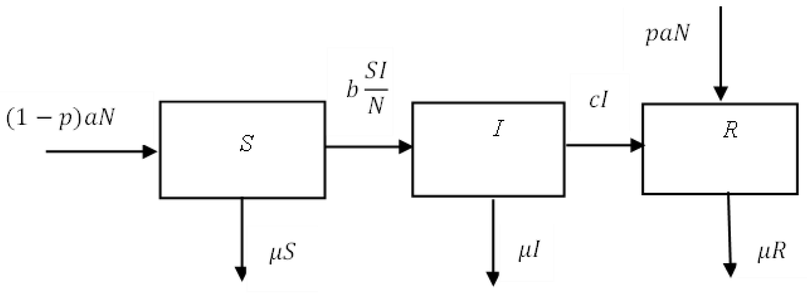
Figure 1. Schematic diagram of the SIR epidemic model.
Technologies 10 00082 g001
Figure 2. RK4 solutions together with the 3-iterations of MNIM and 5-iterations NIM solutions for (a) x ( t ) , (b) y ( t ) , (c) z ( t ) on domain [ 0 , 5 ] of SIR Epidemic Model. NIM solutions are inaccurate as time t gets larger MNIM results are more accurate in the region of large time t (in years) than NIM.
Technologies 10 00082 g002
Figure 3. RK4 solutions together with the 3- iterations of MNIM for x ( t ) , y ( t ) , z ( t ) on time t (in years) domain [ 0 , 10 ] of SIR Epidemic Model. MNIM solutions coincide with the RK4 solutions.
Technologies 10 00082 g003
Table 1. Comparisons of absolute errors between ADM, NIM and MNIM solutions with RK4 for SIR Epidemic Model with respect to time t (in years).
= | R K 4 h = 0.001 A D M |
= | R K 4 h = 0.001 N I M |
= | R K 4 h = 0.001 M N I M |
t
x ( t )
y ( t )
z ( t )
x ( t )
y ( t )
z ( t )
x ( t )
y ( t )
z ( t )
10.00015540.00014620.008530.31680.014890.3021.119 × 10−41.111 × 10−41.286 × 10−5
20.0074250.0068550.13630.17760.024620.20223.705 × 10−43.637 × 10−47.565 × 10−5
30.065940.059780.68920.095310.039120.13484.592 × 10−44.442 × 10−41.518 × 10−4
40.30710.27452.1750.044450.04210.09074.396 × 10−44.188 × 10−42.064 × 10−4
51.0310.91365.3050.0073610.051120.067064.055 × 10−43.817 × 10−42.345 × 10−4
62.8432.514110.082680.060570.066783.849 × 10−43.598 × 10−42.427 × 10−4
76.8656.08120.370.21750.36970.11333.76 × 10−43.504 × 10−42.379 × 10−4
815.0213.3634.79363.9363.90.68093.704 × 10−43.447 × 10−42.249 × 10−4
930.3827.1955.824.648 × 1044.648 × 1046.8343.615 × 10−43.358 × 10−42.071 × 10−4
1057.6451.9385.32.629 × 1062.629 × 10654.193.459 × 10−43.206 × 10−41.864 × 10−4
Publisher’s Note: MDPI stays neutral with regard to jurisdictional claims in published maps and institutional affiliations.