Article

A Quasi-Closed-Form Solution for the Valuation of American Put Options

by
Cristina Viegas
1,* and
José Azevedo-Pereira
2
1
Faculty of Economics, University of the Algarve, CEFAGE (UAlg) Center for Advanced Studies in Management and Economics and Research Centre for Tourism, Sustainability and Well-Being (CinTurs); Campus de Gambelas, Edifício 9, 8005-139 Faro, Portugal
2
ISEG—Lisbon School of Economics and Management, Universidade de Lisboa, Rua Miguel Lupi, 20, 1249-078 Lisboa, Portugal
*
Author to whom correspondence should be addressed.
Int. J. Financial Stud. 2020, 8(4), 62; https://doi.org/10.3390/ijfs8040062
Submission received: 18 September 2020 / Revised: 6 October 2020 / Accepted: 12 October 2020 / Published: 16 October 2020
(This article belongs to the Special Issue Alternative Models and Methods in Financial Economics)

Abstract

:
This study develops a quasi-closed-form solution for the valuation of an American put option and the critical price of the underlying asset. This is an important area of research both because of a large number of transactions for American put options on different underlying assets (stocks, currencies, commodities, etc.) and because this type of evaluation plays a role in determining the value of other financial assets such as mortgages, convertible bonds or life insurance policies. The procedure used is commonly known as the method of lines, which is considered to be a formulation in which time is discrete rather than continuous. To improve the quality of the results obtained, the Richardson extrapolation is applied, which allows the convergence of the outputs to be accelerated to values close to reality. The model developed in this paper derives an explicit formula of the finite-maturity American put option. The results obtained, besides allowing us to quickly determine the option value and the critical price, enable the graphical representation—in two and three dimensions—of the option value as a function of the other components of the model.

1. Introduction

The value of a European option is easily determined by applying the formula derived by Black and Scholes (1973). In turn, the valuation of an American put option seems to be a much more complex task. The possibility of early exercise by the holder of such options is the main obstacle to determining a closed-form solution. It is thus necessary to determine the critical price of the underlying asset, below which the option must be exercised immediately. This calculation represents a major problem in obtaining a closed-form solution. Zhu et al. (2018) report that a closed-form solution is only possible in some special cases. For example, works such as those by Zhu (2006a) and Zhao and Wong (2012) have developed a closed form solution for the optimal exercise boundary and the option price of American put options by using the homotopy analysis method. However, the implementation of the infinite series solution of Zhu (2006a) is a very complex and time-consuming problem, and it requires a recursive procedure of solving differential equations. On the other hand, the application of the homotopy solution by Zhao and Wong (2012) requires a complex iterative integration. Recently, Leipold and Vasiljevic (2017) obtained the prices of American options in closed form in a hyper-exponential jump-diffusion framework. So, almost all the recent work uses a numerical method to solve the problem of pricing American options. For example, Ballestra (2018) develops a numerical method for American option pricing that combines the front-fixing approach and the repeated Richardson extrapolation. The paper shows that the method used yields very accurate and fast results.
Much of the work that has presented analytical solutions for the option price use numerical methods to determine the critical price of the underlying asset. For example, studies such as Kim (1990), Jacka (1991) and Carr et al. (1992), consider that the value of the American option is the value of the European option plus a premium that is given by the discounted value of the potential gains inherent to early exercise. This premium is given by an integral equation, while the exercise boundary is determined by a reversible numerical procedure.
In turn, studies such as Geske and Johnson (1984), Bunch and Johnson (1992), Ho et al. (1994), Huang et al. (1996) and Lee and Paxson (2003) develop analytical approximations for the American put option price by calculating the values of sets of options with discrete exercise dates. Based on the properties discussed in Geske and Johnson (1984) and Kim (1990), Fabozzi et al. (2016) present the extension method. In this method, they develop a quasi-analytic approach that aims to improve the performance of existing methods in calculating the value of American options with long maturities.
In parallel, there are works that, by presenting analytical formulations for the price of American put options, explicitly determine the critical price of the underlying asset. Particularly prominent in this area is the work of Carr and Faguet (1996), Carr (1998) and Bunch and Johnson (2000), which offer significant advances in the calculation of the value of American put options using quasi-explicit solutions. For example, the derivation of an expression for the so-called critical price of the underlying asset of an American put option is one of the main objectives of Bunch and Johnson (2000). Once the value of this variable has been determined, the authors use it to determine the value of the American put option, using the method proposed in Huang et al. (1996). It should, however, be noted that the Bunch and Johnson (2000) solution is only valid for American put options whose underlying asset does not distribute dividends. Another reference in the field of analytical approximations for the critical stock prices of American options is Zhu (2006b). This article proposed a method based on the Laplace transform of the fundamental valuation partial differential equation. However, Li (2010) shows that the technique presented in Zhu (2006b) gives very inaccurate results to the critical stock price, being that the Average Percentage Error is comprised between 8 and 9%.
Two other reference works are those of Carr and Faguet (1996) and Carr (1998). These two studies transform the general partial differential equation (the equation given by Black and Scholes (1973), which was the basis for determining the value of the European option on the stock) into a non-homogeneous ordinary differential equation. This change implies the replacement of the derivative of price function with respect to time by a finite difference. The basic assumptions for the application of this procedure are different in the two articles. Thus, Carr (1998) justifies his procedure by classifying time as random and considering that it follows an Erlang or gamma distribution. Carr and Faguet (1996), by contrast, report that obtaining an analytical solution requires the implementation of the method of lines, which means that the time component of the model ceases to be continuous and becomes discrete.
This article focuses on the development of an analytical solution capable of evaluating an American put option, assuming that the underlying asset distributes dividends. This is an important area of research both because of a large number of transactions for American put options on different underlying assets (stocks, currencies, commodities, etc.) and because this type of evaluation plays a role in determining the value of other financial assets such as mortgages, convertible bonds or life insurance policies.
In this study, the method of lines is followed; this is considered to be a formulation in which time is discrete rather than continuous. This method was used in the evaluation of options by Carr and Faguet (1996) and Meyer and Hoek (1997). The former study used this method to derive an exact valuation formula for perpetual options subject to a finite series of credit downgrades, which can be used to approximate the value of finite-lived American options. The later takes a numerical approximation to calculate the value of an American option. The model developed in this paper represents a contribution to the existing literature on the application of the method of lines to calculate the value of the American put option, once it is derived an explicit formula of the finite-maturity American put option.
The remainder of this paper is organized as follows. Section 2 develops a model to evaluate American put options in which the underlying asset pays dividends, a closed-form solution being reached for the case of constant dividends and a quasi-closed-form solution where the dividends are proportional to the value of the underlying asset. In Section 3, the results obtained by applying the formulas derived in the previous section are presented numerically and graphically. They are also compared with other values obtained by different authors who have presented work in this area of research. Finally, the conclusion is presented, including suggestions for future developments.

2. The American Put Option Valuation Model

2.1. Analytical Solution for the Value of an American Put Option

The model presents two variants: constant dividends, ϕ , and dividends in proportion to the price of the underlying asset, δ . In the case of constant dividends, the model developed in this work allows obtaining a closed form solution to the American put option price, while for dividends in proportion to the value of the underlying asset, the model allows only to reach a quasi-explicit solution, since the critical price is only liable to be found numerically.
In the case of constant dividends, it is assumed that the initial value of the underlying asset is liable to be decomposed by the following expression, following Roll (1977):
S = s + ϕ r ( 1 e r τ )
where the second term on the right hand side corresponds to the updated value, in continuous time, of the fixed component of the future flow of dividends receivable in the period τ, r represents the interest rate, and s the sum of the updated value of the variable component of dividends receivable in the period τ and the updated value of all dividends expected to be received after that period.
In the formulation developed in this study, time is considered to be discrete, whereby (1) is replaced by the following configuration:
S = s + D
where
D = ϕ τ n 1 1 ( 1 + r τ n ) n r τ n
D represents the updated value of an income with n constant terms, which means that the continuing value of the fixed component of the dividends has been replaced by n discrete values equal to ϕ τ n each one, with a time period between two consecutive terms equal to τ n . The total period of time of the possession of the instrument is equal to τ. The expression (2) may also present a simpler configuration:
S = s + ϕ r ( 1 1 ( 1 + r τ n ) n )
After these initial considerations relating to the form in which the fixed component of the future flow of dividends receivable in the period τ should be considered in the valuation process, the development of a methodology to determine the value of an American put option on an asset that pays dividends begins. From here, the formulas to present consider, alternatively, constant dividends, ϕ , or dividends in proportion to the underlying asset, δ . In other words, for steady dividends, we have δ = 0 and ϕ 0 , while for proportional dividends, ϕ = 0 and δ 0 are considered. In contrast, the whole formulation used for this purpose is a function of s, the underlying asset price minus the updated value of the fixed component of the dividends expected to be received during the period τ .
The process to be developed is based on the technique used for the valuation of contingent claims. It is considered that the option value depends on a single stochastic variable: the price of the underlying asset. The evolution of this variable is defined according to the following stochastic process:
d s = ( r δ ) s d t + σ s s d z s
where r represents the short-term risk-free interest rate, δ the rate of dividend distribution, σ s the instantaneous standard deviation and z s the standard Wiener process.
Considering that the option value, P ( s , τ ) , depends on the stochastic variable—the price of the underlying asset—and that it follows the process defined in (4), the partial differential equation may be deduced:
P ( τ , s ) τ + P ( τ , s ) s ( r δ ) s + 1 2 σ S 2 s 2 2 P ( τ , s ) s 2 r P ( τ , s ) = 0   if s s m _
where s m _ corresponds to the critical value, the underlying asset price, less the updated value of the fixed component of the dividends expected to be received during the period τ .
Note that, as with the underlying asset price, the following equality is also checked within the critical price:
S m _ = s m _ + ϕ r ( 1 1 ( 1 + r τ n ) n )
The method to be developed lies in the transformation of the general partial differential equation into a non-homogeneous ordinary differential equation. This change is made by applying the method of lines. It involves replacing the derivative of the price function, with respect to time, by a finite difference, while the derivatives in relation to the prices of the underlying asset remain unchanged. This process results in a sequence of non-homogeneous ordinary differential equations that must be solved. The shorter the time interval considered in the finite difference, the higher the quality of the results reached with this change. So, to attain a good estimation of the value of the option, it would be convenient to consider time as being divided into a number of intervals tending towards infinity. However, a big number of time intervals means a significant increase in mathematical computation. Thus, there is a tendency to use a relatively small number of time intervals, and then the Richardson extrapolation is applied (the Richardson extrapolation has been applied to studies in the area with success; see, for example, Carr (1998)) in order to accelerate the convergence of the results obtained to values close to reality. For example, Carr and Faguet (1996) and Carr (1998) show that the subdivision of the total time of ownership of the option into four intervals leads to very acceptable estimates. So, in this paper, time is subdivided into four intervals.
Thus, Equation (5) takes on the following general configuration for s s m _ :
d P ( m ) ( s ) d s ( r δ ) s + 1 2 σ S 2 s 2 d 2 P ( m ) ( s ) d s 2 r P ( m ) ( s ) = P ( m ) ( s ) P ( m 1 ) ( s ) τ n
P ( m ) ( s ) corresponds to the value of the option and m corresponds to the number of sub-periods in relation to the total number of time intervals, n = 4 , considered under the model. Thus, the expression of the value of the American put option is determined, relative to m τ n periods of time, with m = 1 , 2 , 3 , 4 and m n .
So, (7) is a non-homogeneous ordinary differential equation in which the option price becomes a function of a single variable.
To determine P ( m ) ( s ) , we need to know the expression of P ( m 1 ) ( s ) , whereby this equation must be solved for m = 1, 2, 3, 4.
The value of the American put option should confirm (7) in conjunction with the following boundary conditions:
lim s P ( m ) ( s ) = 0
lim s s m _ P ( m ) ( s ) = K S m _
lim s s m _ d P ( m ) ( s ) d s = 1
where K corresponds to the strike price.
To achieve the objective of determining the value of the American put option, by solving (7), subject to the restrictions (8–10), the procedure used in studies such as Huang et al. (1996) applies, where the value of the American option is the value of the European put plus a term that represents the early exercise premium of the American put.
Thus:
P ( m ) ( s ) = p ( m ) ( s ) + p r ( m ) ( s )   if s s m _
where p ( m ) ( s ) is the value of the European put and p r ( m ) ( s ) corresponds to the value of the early exercise premium of the American put.
In turn, the European put option should confirm (7) and the following boundary conditions:
p ( m ) ( s ) = max ( K S , 0 )   for   τ = 0
lim s 0 p ( m ) ( s ) = K ( 1 + r τ n ) n
lim s p ( m ) ( s ) = 0
The respective early exercise premium should confirm (7) and the following condition:
lim s p r ( m ) ( s ) = 0
By using this procedure, the general closed-form solution for the value of the American put option is given by different expressions, according to the range of variation in the price of the underlying asset.
Thus, for s K , m = 1 , 2 , 3 , 4 , n = 1 , 2 , 3 , 4 and m n , the solution of (7), subject to the restrictions (12), (13), and (14), leads to the value of the European put option:
p [ s K ] ( m ) ( s ) = s 2 τ δ + β α n 2 τ σ 2 [ ( a m + 2 n a m 1 ( τ σ 2 α n + ln ( s ) α n ) ) + 2 n 2 a m 2 ( ln ( s ) α n + 2 τ σ 2 α n ) 2 + n 4 a m 3 3 ( 30 τ 3 σ 6 α n 3   + 30 τ 2 σ 4 ln ( s ) α n 5 2 + 9 σ 2 τ ln ( s ) 2 α n 2 + ln ( s ) 3 α n 3 2 ) ]
where:
  • α n = ( 2 r τ + τ σ 2 ) 2 + 4 δ τ 2 ( 2 r + δ + σ 2 ) + 8 n σ 2 for n = 1 , 2 , 3 , 4
  • β = τ σ 2 2 r τ
  • a m i is a parameter with a m i = 0 for mi ≤ 0 and i = 1,2,3.
The same reasoning is followed to determine the value of the early exercise premium, which must confirm the boundary condition defined in (15). Thus, for s s 1 _ , m = 1 , 2 , 3 , 4 , n = 1 , 2 , 3 , 4 and m n , the value of the premium is:
p r ( m ) ( s ) = s 2 τ δ + β α n 2 τ σ 2 [ ( d m + 2 n d m 1 ( τ σ 2 α n + ln ( s ) α n ) ) + 2 n 2 d m 2 ( ln ( s ) α n + 2 τ σ 2 α n ) 2 + n 4 d m 3 3 ( 30 τ 3 σ 6 α n 3   + 30 τ 2 σ 4 ln ( s ) α n 5 2 + 9 σ 2 τ ln ( s ) 2 α n 2 + ln ( s ) 3 α n 3 2 ) ]
where:
  • d m i is a parameter with d m i = 0   for   m i 0   and   i = 1 , 2 , 3 .
Thus, it is possible to present the general solution in relation to the value of the American put option, when s K and m = 1 , 2 , 3 , 4 :
P [ s K ] ( m ) ( s ) = p [ s K ] ( m ) ( s ) + p r ( m ) ( s )
In the region s 1 _ s K , the value of the American put option also corresponds to the European option plus the premium, with the peculiarity that, in this area, the value of the European option to be determined is the call. The first step in solving (7) comprises of determining the option value at the time of the termination of the contract. This value corresponds to the payoff of the option, which is equal to zero in the out-of-money area of a European option. Thus, in the area s 1 _ s K and for τ = 0 , the value of a European call is equal to zero.
The put-call parity being subsequently applied to obtain the expression of the European put. In turn, the value of the premium is configured as defined in (17). Accordingly, the value of the European put, in the region s 1 _ s K , with m = 1 , 2 , 3 , 4 , n = 1 , 2 , 3 , 4 and m n , is given by the following expression (again, the value of a European put must confirm the boundary conditions defined in (12)–(14)):
p [ s 1 _ s K ] ( m ) ( s ) = s 2 τ δ + β + α n 2 τ σ 2 [ ( b m + 2 n b m 1 ( τ σ 2 α n ln ( s ) α n ) ) + 2 n 2 b m 2 ( ln ( s ) α n 2 τ σ 2 α n ) 2 + n 4 b m 3 3 ( 30 τ 3 σ 6 α n 3   30 τ 2 σ 4 ln ( s ) α n 5 2 + 9 σ 2 τ ln ( s ) 2 α n 2 ln ( s ) 3 α n 3 2 ) ] + K ( 1 + r τ n ) m s ( 1 + δ τ n ) m + e m
where b m i is a parameter with b m i = 0 for mi ≤ 0 and i = 1,2,3.
Whereby, the general expression for the amount of the American put option, when s 1 _ s K and m = 1 , 2 , 3 , 4 , is given by:
P [ s 1 _ s K ] ( m ) ( s ) = p [ s 1 _ s K ] ( m ) ( s ) + p r ( m ) ( s )
For s s 1 _ , the option value is given by different expressions according to the range of variation of the price of the underlying asset. Thus, for s 2 _ s s 1 _ , m = 2 , 3 , 4 , n = 2 , 3 , 4 and m n , we have:
P [ s 2 _ s s 1 _ ] ( m ) ( s ) = s 2 τ δ + β + α n 2 τ σ 2 [ z m 1 + 2 n z m 2 ( τ σ 2 α n ln ( s ) α n ) +   2 n 2 z m 3 ( ln ( s ) α n 2 τ σ 2 α n ) 2 ] + K ( 1 + r τ n ) m 1 s ( 1 + δ τ n ) m 1   ϕ ( 1 1 ( 1 + r τ n ) n ) r ( 1 + r τ n ) m 1 +   s 2 τ δ + β α n 2 τ σ 2 [ y m 1 + 2 n y m 2 ( τ σ 2 α n + ln ( s ) α n ) +   2 n 2 y m 3 ( ln ( s ) α n + 2 τ σ 2 α n ) 2 ]
where y m i and z m i are parameters with y m i and z m i for m i n and i = 2,3.
In turn, for s 3 _ s s 2 _ , m = 3 , 4 , n = 3 , 4 and m n , the formula for the value of the American put option is as follows:
P [ s 3 _ s s 2 _ ] ( m ) ( s ) = s 2 τ δ + β + α n 2 τ σ 2 ( w m 2 + 2 n w m 3 ( τ σ 2 α n ln ( s ) α n ) ) + K ( 1 + r τ n ) m 2   s ( 1 + δ τ n ) m 2   ϕ ( 1 1 ( 1 + r τ n ) n ) r ( 1 + r τ n ) m 2 + s 2 τ δ + β α n 2 τ σ 2 ( x m 2 + 2 n x m 3 ( τ σ 2 α n + ln ( s ) α n ) )
where w m i and x m i are parameters with w m i = 0   and   x m i = 0   for   m i 0   and   i = 3 .
For the area s 4 _ s s 3 _ , m = 4 and n = 4 , the option value corresponds to:
P [ s 4 _ s s 3 _ ] ( m ) ( s ) = u 1 s 2 τ δ + β + α n 2 τ σ 2 + K 1 + r τ n   s 1 + δ τ n ϕ ( 1 1 ( 1 + r τ n ) n ) r ( 1 + r τ n )   + v 1 s 2 τ δ + β α n 2 τ σ 2
where u 1 and v 1 are parameters. Finally, for s s m _ , with m = 1 , 2 , 3 , 4 and m = n , the American put option is exercised immediately, whereby its value corresponds to:
P [ s s m _ ] ( m ) ( s ) = K S
These different expressions for the value of the American put option contain a set of parameters ( a m i , d m i , b m i , y m i , z m i , w m i , x m i , u 1 , v 1 ) whose value is determined by solving a system of equations.
For m = 1 , 2 , 3 , 4 , n = 1 , 2 , 3 , 4 , m n and s = K :
p [ s K ] ( m ) ( s ) = p [ s 1 _ s K ] ( m ) ( s )
d p [ s K ] ( m ) ( s ) d s = d p [ s 1 _ s K ] ( m ) ( s ) d s
d 2 p [ s K ] ( m ) ( s ) d s 2 = d 2 p [ s 1 _ s K ] ( m ) ( s ) d s 2
For m = 1 , n = 1 , 2 , 3 , 4 and s = s 1 _ :
P [ s 1 _ s K ] ( m ) ( s ) = P [ s s 1 _ ] ( m ) ( s )
For m = 2 , 3 , 4 ,   n = 2 , 3 , 4 , m n and s = s 1 _ :
P [ s 2 _ s s 1 _ ] ( m ) ( s ) = P [ s 1 _ s K ] ( m ) ( s )
d P [ s 2 _ s s 1 _ ] ( m ) ( s ) d s = d P [ s 1 _ s K ] ( m ) ( s ) d s
For m = 2 , 3 , 4 , n = 2 , 3 , 4 , m n and s = s n _
P [ s s n _ ] ( m ) ( s ) = P [ s n _ s s n 1 _ ] ( m ) ( s )
For m = 3 , 4 , n = 3 , 4 , m n and s = s 2 _
P [ s 2 _ s s 1 _ ] ( m ) ( s ) = P [ s 3 _ s s 2 _ ] ( m ) ( s )
d P [ s 2 _ s s 1 _ ] ( m ) ( s ) d s = d P [ s 3 _ s s 2 _ ] ( m ) ( s ) d s
For s = s 4 _ :
P [ s 4 _ s s 3 _ ] ( 4 ) ( s ) = K s 4 _ ϕ r ( 1 1 ( 1 + r τ n ) n )
d P [ s 4 _ s s 3 _ ] ( 4 ) ( s ) d s = 1
To determine the value s 1 _ , the following equation must be solved for s = s 1 _ and n = 1 , 2 , 3 , 4 :
d P [ s 1 _ s K _ ] ( 1 ) ( s ) d s = 1
For δ 0 , the value s 1 _ is given implicitly and must be found numerically (for numerical resolution, Maple software with “fsolve” was used). For δ = 0 and ϕ 0 , the value s 1 _ is calculated as follows:
s 1 _ = exp ( σ 2 τ ( ln ( 4 b 1 2 r 2 ( n + r τ ) 2 α n ( β + α n ) 2 ( ϕ n ϕ ( n + r τ n ) n n + ϕ r τ + K r 2 ( n + r τ n ) n τ ϕ ( n + r τ n ) n r τ ) 2 ) + 2 n ln ( n + r τ n ) ) β α n )
Whereby the critical value is equal to:
S 1 _ = s 1 _ + ϕ r ( 1 1 ( 1 + r τ n ) n )
In turn, for the value s = s m _ , m = 1 , 2 , 3 , 4 and n = 2 , 3 , 4 , the value of s m _ is determined by solving the following equation:
d P [ s m _ s s m 1 _ ] ( m ) ( s ) d S = 1
An explicit expression is only reached when one considers ϕ 0   and   δ = 0 , as had already happened in the previous deduction, for s 1 _ . For δ 0 , the value s m _ is determined numerically.
Accordingly, for ϕ 0   and   δ = 0 :
s m _ = exp ( σ 2 τ ( ln ( 4 γ 2 ( n + r τ ) 2 α n τ 2 ( K r ( n + r τ n ) n ϕ ( n + r τ n ) n + ϕ ) 2 ( β + α n ) 2 ) + 2 n ln ( n + r τ n ) ) β α n )
where, for m = 2 we have γ = z m 1 , for m = 3 we have γ = w m 2 , and for m = 4 we have γ = u 1 .
In accordance with the foregoing, the critical value is equal to:
S m _ = s m _ + ϕ r ( 1 1 ( 1 + r τ n ) n )

2.2. The Application of the Richardson Extrapolation in the Valuation Model of an American Put Option

In this article, despite considering time as being divided into a relatively small number of sub-periods, a good estimate can be made of the value of an American put option by applying the Richardson extrapolation.
In this context, it is considered that the figures for the American put option obtained from the equations specified in advance, for n = 1 , 2 , 3 , 4 , are functions of the sub-periods of time applied in each case, i.e., of τ , τ 2 , τ 3 , τ 4 , respectively. These functions are designated by P ^ ( τ n ) , with n = 1 , 2 , 3 , 4 .
According to Carr (1998), the use of the Richardson extrapolation is appropriate given that the function P ^ ( τ n ) can be represented by the Maclaurin series:
P ^ ( τ n ) = P ^ ( 0 ) + τ n P ^ ( 0 ) + ( τ n ) 2 2 ! P ^ ( 0 ) + + ( τ n ) n n ! P ^ ( n ) ( 0 ) + O ( ( τ n ) n )
where O ( ( τ n ) n ) represents the approximation error, which tends towards zero when n tends towards infinity. The extrapolated value of the American put option corresponds to the solution of P ^ ( 0 ) . In order for this result to be possible to achieve, the following is considered:
P ^ ( τ n ) P ^ ( 0 ) + τ n P ^ ( 0 ) + ( τ n ) 2 2 ! P ^ ( 0 ) + ( τ n ) 3 3 ! P ^ ( 0 )
Considering n = 1 , n = 2 , n = 3   and   n = 4 , (38) is transformed into a system of four equations with four variables, P ^ ( 0 ) , P ^ ( 0 ) , P ^ ( 0 )   and   P ^ ( 0 ) . The resolution of this system allows the extrapolated value of the American put option to be found:
P ^ ( 0 ) = 32 3 P ^ ( τ 4 ) 27 2 P ^ ( τ 3 ) + 4 P ^ ( τ 2 ) 1 6 P ^ ( τ )
The same kind of reasoning should be applied to determining the extrapolated critical value of the underlying asset:
S ^ 4 _ ( 0 ) = 32 3 S ^ 4 _ ( τ 4 ) 27 2 S ^ 3 _ ( τ 3 ) + 4 S ^ 2 _ ( τ 2 ) 1 6 S ^ 1 _ ( τ )
With the application of the Richardson extrapolation, the extrapolated values of the critical price, S ^ 4 _ ( 0 ) , and of the American put option, P ^ ( 0 ) , are determined, which allows a very satisfactory approximation to the value of these functions to be obtained, despite only sub-periods being considered.

3. Results of the American Put Option Valuation Model

This section presents and discusses, numerically and graphically, the results provided by the American put option general valuation model, as described above. This analysis is carried out through the presentation of graphs representing the evolution of the option value, as well as tables where numerical figures are shown for the value of the American put option.
The aim is thus to show that the formulas described herein relating to the valuation of the American put option represent a good estimate of the option value compared with those presented in other studies in the area. Thus, the results obtained for the American put option using the formulas derived in this study are compared with other values that have been reached by different authors in studies undertaken in this research area.
There are studies, specifically Ju (1998), that determine the root of the mean squared absolute errors. In this study, and following Lee and Paxson (2003), the root of the mean squared relative errors is determined, which means that the weighting is based on the absolute errors by the option value. In the following tables, in addition to the value of the American put option being shown, the root of the mean squared relative errors, R M S R E , is also determined:
R M S R E = 1 n i = 1 n [ ( P ( A ) i P i ) / P i ] 2
where n is the total number of options analyzed, P ( A ) i corresponds to the approximate option value i and P i corresponds to the reference option value i .
In Table 1, the values of an American put option are calculated for different price levels of the underlying asset and for different rates of dividend distribution. In Table 2, the values of an American put option are calculated for different price levels of the underlying asset, different terms, different levels of price volatility of the underlying asset, different interest rates and different rates of dividend distribution. Note that the MLE results (n = 4) are the values obtained according to the model developed in this study using the Richardson extrapolation with four-time intervals.
An analysis of the tables shows that the approach developed in this study provides a good estimate compared with the values obtained by other studies referenced in the tables. An analysis of Table 1 shows that the values obtained with the model proposed herein are identical to those obtained by Carr (1998), provided that the same number of time intervals is considered. Table 2 shows that the approach used in this study results in a smaller deviation from the reference values. This is even more noticeable for longer-term options.
Figure 1 shows, in three dimensions, the evolution of the value of the American put option in the case of constant dividends, where the price of the underlying asset and time to maturity vary. The surface with a straight slope, relating to the lowest values of the underlying asset, represents the immediate exercise of the option area. In turn, the intermediate surface, convex and with a steeper slope, relates to the area where the underlying asset is below the exercise price, but higher than the critical price. It seems that, in this area, the option value is more sensitive to changes in the price of the underlying asset compared with what happens when the underlying asset has greater values than the exercise price, the area represented by the flatter surface. Another point to mention is the behavior of the option price when the time to maturity varies. The option value shows a slight tendency to increase as maturity increases. When the price of the underlying asset approaches the critical value, the option value is more sensitive to variations in maturity.
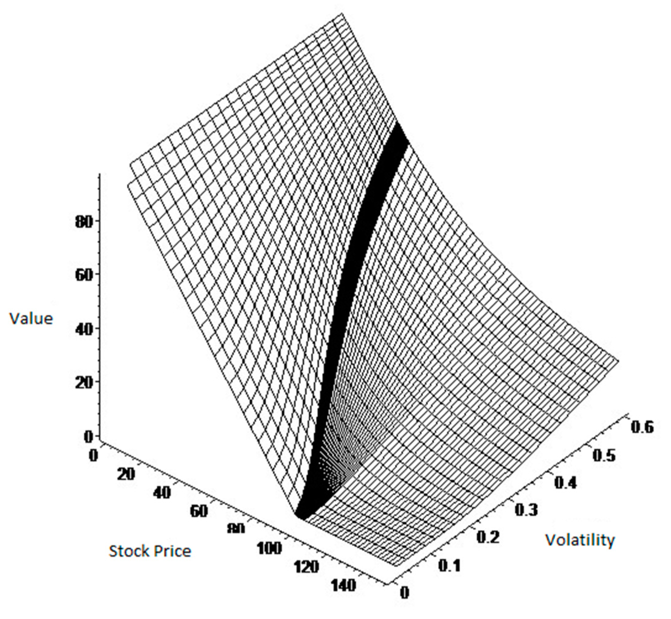
Figure 2 shows the option value, in the case of constant dividends, as a function of the price of the underlying asset and the volatility of that price. As in Figure 1, the behavior of the option value is divided into three distinct zones showing a similar evolution to that mentioned earlier in terms of the relationship between the underlying asset and the option value. By contrast, it appears that the greater the volatility in the price of the underlying asset, the higher the option price is. This is most significant when nearing the critical value. Another aspect that emerges from analyzing the diagram is that the critical price tends to decrease significantly as the volatility of the underlying asset increases. By contrast, it is notable in both graphs that positive changes in the price of the underlying asset causes a decrease in the option value.
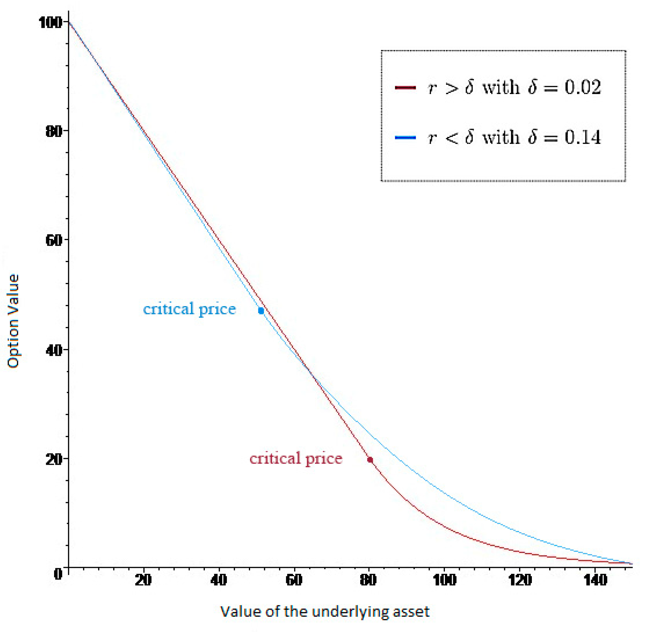
Figure 3 shows, in two dimensions, the evolution of the price of the American put option as a function of the value of the underlying asset. In formulating this graph, consider the existence of dividends in proportion to the value of the underlying asset and time divided into four intervals. It can be seen that for values of the underlying asset are lower than the critical price, the option value is represented by a straight line with a negative slope and for values greater than the critical value, the configuration of the graph is a convex curve. By contrast, it seems that as the price of the underlying asset increases, the option value approaches zero. It also can be observed that all other parameters remaining unchanged, when the dividend rate increases, the critical price decreases.
The presentation and comparison of these numerical results demonstrate that the closed-form solution, or the quasi-closed-form solution described herein, is a credible alternative for the valuation of such derivatives.

4. Conclusions

This paper has developed a model of calculating American put options that is capable of improving current practices. The sharp increase in such contracts over the past two decades justifies the increased academic effort placed into developing models appropriate for their valuation. In most cases, the literature on this subject has provided only numerical solutions for this type of valuation framework. In order to arrive at these same numerical solutions, it is necessary to use complex computing techniques, a fact that makes the process overly time-consuming and costly.
The model described in this paper presents two variants. For the case of constant dividends, a closed-form solution for the option value and the respective critical price is obtained. In the case of dividends in proportion to the value of the underlying asset, a quasi-closed-form solution is obtained, since the critical price is determined numerically. These results, besides allowing us to quickly determine the option value and the critical price, enable the graphical representation—in two and three dimensions—of the option value as a function of the other components of the model. This numerical and graphical analysis allows us to conclude that the model proposed herein provides results that are consistent with financial reality.
This work aims to contribute to an area of financial investigation until now largely unexplored: the development of closed-form solutions for the valuation of American put options. Based on this work, it is possible to identify a number of suggestions for future developments. The formulation developed throughout the paper considers time divided into four intervals when the change is made from continuous to discrete time. It would be desirable to develop a general formula that may be applied to any number of time intervals. Another, more ambitious improvement that may be suggested is to develop a model for the two variants of the model in which the option value and the critical price are given by an analytical solution in continuous time. In such a situation, it would be unnecessary to apply the Richardson extrapolation.

Author Contributions

Conceptualization, C.V. and J.A.-P.; methodology, C.V.; software, C.V.; validation, C.V. and J.A.-P.; formal analysis, C.V. and J.A.-P.; investigation, C.V. and J.A.-P.; resources, C.V. and J.A.-P.; writing—original draft preparation, C.V.; writing—review and editing, C.V. and J.A.-P.; visualization, C.V. and J.A.-P.; funding acquisition, C.V. All authors have read and agreed to the published version of the manuscript.

Funding

This research was funded by FCT- FOUNDATION FOR SCIENCE AND TECHNOLOGY, within the project UIDB/04007/2020.

Acknowledgments

The authors thank the referees for their valuable suggestions and remarks which improved the paper.

Conflicts of Interest

The authors declare no conflict of interest. The funders had no role in the design of the study; in the collection, analyses, or interpretation of data; in the writing of the manuscript, or in the decision to publish the results.

References

  1. Aitsahlia, Farid, and Peter Carr. 1997. American options: A comparison of numerical methods. In Numerical Methods in Finance. Edited by Leonard Christopher Gordon Rogers and Denis Talay. Cambridge: Cambridge University Press, pp. 67–87. [Google Scholar]
  2. Ballestra, Luca Vincenzo. 2018. Fast and accurate calculation of American option prices. Decisions in Economics and Finance 41: 399–426. [Google Scholar] [CrossRef]
  3. Bjerksund, Petter, and Gunnar Stensland. 1993. Closed-form approximation of American options. Scandinavian Journal of Management 9: 87–99. [Google Scholar] [CrossRef]
  4. Black, Fischer, and Myron Scholes. 1973. The pricing of options and corporate liabilities. Journal of Political Economy 81: 637–59. [Google Scholar] [CrossRef] [Green Version]
  5. Bunch, David, and Herb Johnson. 1992. A simple and numerically efficient valuation method for American puts using a modified Geske-Johnson approach. Journal of Finance 47: 809–816. [Google Scholar]
  6. Bunch, David, and Herb Johnson. 2000. The American put option and its critical stock price. Journal of Finance 55: 2333–56. [Google Scholar] [CrossRef]
  7. Carr, Peter. 1998. Randomization and the American put. The Review of Financial Studies 11: 597–626. [Google Scholar] [CrossRef]
  8. Carr, Peter, and Dmitri Faguet. 1996. Valuing Finite-Lived Options as Perpetual. SSRN Electronic Journal. Available online: https://papers.ssrn.com/sol3/papers.cfm?abstract_id=706 (accessed on 6 October 2020).
  9. Carr, Peter, Robert Jarrow, and Ravi Myneny. 1992. Alternative characterizations of American put options. Mathematical Finance 2: 87–106. [Google Scholar] [CrossRef]
  10. Fabozzi, Frank J., Tommaso Paletta, Silvia Stanescu, and Radu Tunaru. 2016. An improved method for pricing and hedging long dated American options. European Journal of Operational Research 254: 656–66. [Google Scholar] [CrossRef]
  11. Fatone, Lorella, Francesca Mariani, Maria Cristina Recchioni, and Francesco Zirilli. 2015. The Barone-Adesi Whaley formula to price American options revisited. Applied Mathematics 6: 382–402. [Google Scholar] [CrossRef] [Green Version]
  12. Geske, Robert, and Herb E. Johnson. 1984. The American put valued analytically. Journal of Finance 39: 1511–24. [Google Scholar] [CrossRef]
  13. Ho, Thomas S., Richard Christopher Stapleton, and Marti Gurunath Subrahmanyam. 1994. A Simple technique for the valuation and hedging of American options. Journal of Derivatives 2: 52–66. [Google Scholar] [CrossRef]
  14. Huang, Jing-zhi, Marti Gurunath Subrahmanyam, and G. George Yu. 1996. Pricing and hedging American options: A recursive integration method. The Review of Financial Studies 9: 277–300. [Google Scholar] [CrossRef]
  15. Ingersoll, Jonathan E., Jr. 1998. Approximating American options and other financial contracts using barrier derivatives. Journal of Computational Finance 2: 85–112. [Google Scholar] [CrossRef]
  16. Jacka, Saul D. 1991. Optimal stopping and the American put. Mathematical Finance 1: 1–14. [Google Scholar] [CrossRef]
  17. Ju, Nengjiu. 1998. Pricing an American option by approximating its early exercise boundary as a multipiece exponential function. Review of Financial Studies 11: 627–46. [Google Scholar] [CrossRef]
  18. Kim, In Joon. 1990. The analytic valuation of American puts. Review of Financial Studies 3: 547–72. [Google Scholar] [CrossRef]
  19. Lee, Jongwoo, and Dean Paxson. 2003. Confined exponential approximations for the valuation of American options. The European Journal of Finance 9: 1–26. [Google Scholar] [CrossRef]
  20. Leipold, Markus, and Nikola Vasiljevic. 2017. Pricing and disentanglement of American puts in the hyper-exponential jump-diffusion model. Journal of Banking and Finance 77: 78–94. [Google Scholar] [CrossRef]
  21. Li, Minqiang. 2010. Analytical approximations for the critical stock prices of American options: A performance comparison. Review of Derivatives Research 13: 75–99. [Google Scholar] [CrossRef]
  22. Meyer, Gunter H., and John van der Hoek. 1997. The valuation of American options with the method of lines. In Advances in Futures and Options Research. Edited by Phelim Boyle, George Pennacchi and Peter Ritchken. Bingley: Emerald Group Publishing Limited, pp. 265–85. [Google Scholar]
  23. Roll, Richard. 1977. An analytic valuation formula for unprotected American call options on stocks with known dividends. Journal of Financial Economics 5: 251–58. [Google Scholar] [CrossRef]
  24. Zhao, Jing, and Hoi Ying Wong. 2012. A closed-form solution to American options under general diffusion processes. Quantitative Finance 12: 725–37. [Google Scholar] [CrossRef]
  25. Zhu, Song-Ping. 2006a. An exact and explicit solution for the valuation of American put options. Quantitative Finance 6: 229–42. [Google Scholar] [CrossRef]
  26. Zhu, Song-Ping. 2006b. A new analytical-approximation formula for the optimal exercise boundary of American put options. International Journal of Theoretical and Applied Finance 9: 1141–77. [Google Scholar] [CrossRef]
  27. Zhu, Song-Ping, Xin-Jiang He, and Xiaoping Lu. 2018. A new integral equation formulation for American put options. Quantitative Finance 18: 483–90. [Google Scholar] [CrossRef] [Green Version]
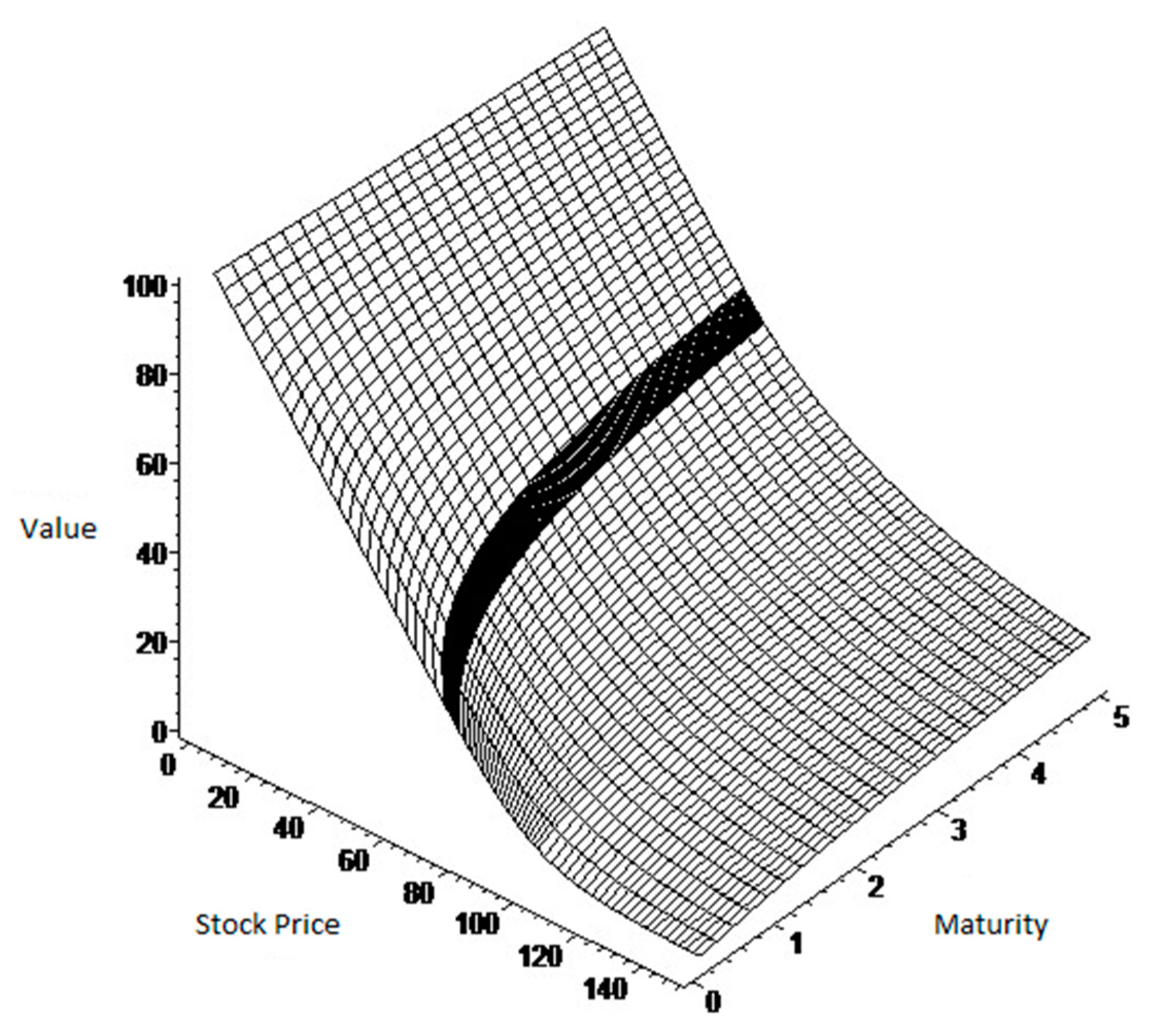
Figure 1. American put option as a function of S and τ. The values of the parameters underlying the construction of this figure are as follows: n, the number of time intervals is 2; r, the interest rate is 0.06; σ, the volatility of the stock price is 0.4; K, the strike price is 100; and ϕ, the value of constant dividends is 1.6.
Ijfs 08 00062 g001
Figure 2. American put option as a function of S and σ. The values of the parameters underlying the construction of this figure are as follows: n, the number of time intervals is 2; r, the interest rate is 0.06; τ, the term remaining to maturity is 3 years; K, the strike price is 100; and ϕ, the value of constant dividends is 1.6.
Ijfs 08 00062 g002
Figure 3. American put option as a function of S . The values of the parameters underlying the construction of this figure are as follows: n , the number of time intervals is 4; τ , the term remaining to maturity is 3 years; r , the interest rate is 0.08; σ , the volatility of the stock price is 0.20; K , the strike price is 100; S 4 _ , the critical price is 79.66; δ , the rate of dividend distribution is 0.02 and 0.14; and, ϕ , the value of constant dividends is 0.0.
Ijfs 08 00062 g003
Table 1. Comparison of American put option values ( τ = 3 ).
(1)
(S; δ)
(2)
TRUE
(3)
RAN4
(4)
EXP3
(5)
QD+
(6)
QD*
(7)
PA
(8)
MLE (n = 4)
(80;0.12)25.65825.65425.65725.75325.71525.64825.654
(90;0.12)20.08320.08420.08220.20220.17620.07920.084
(100;0.12)15.49815.49815.49715.61815.60115.50915.498
(110;0.12)11.80311.80511.80211.91211.90011.83411.805
(120;0.12)8.8868.8858.8858.9788.9708.9418.885
(80;0.08)22.20522.19722.20822.16222.14922.19622.197
(90;0.08)16.20716.19716.21116.18116.1716.19416.197
(100;0.08)11.70411.68811.70711.70811.711.69211.688
(110;0.08)8.3678.3548.378.3958.398.368.354
(120;0.08)5.935.9185.9325.9715.9675.9295.918
(80;0.04)20.3520.3520.35120.33420.33720.34220.35
(90;0.04)13.49713.49613.513.46513.47113.47313.496
(100;0.04)8.9448.9368.9478.9268.9318.9128.936
(110;0.04)5.9125.9025.9155.9165.925.8765.902
(120;0.04)3.8983.8873.93.923.9223.863.887
(80;0.00)20202020202020
(90;0.00)11.69711.70111.69911.70311.70911.70111.701
(100;0.00)6.9326.9326.9356.956.9586.9146.932
(110;0.00)4.1554.1534.1574.1854.1914.1324.153
(120;0.00)2.512.5072.5122.5482.5512.4842.507
R M S R E -0.001050.000320.005900.005870.004130.00105
S is the underlying asset price and δ is the rate of dividend distribution. Columns 2–4 are taken from Ju (1998): the “TRUE” value is based on the binomial tree model with N = 10.000 time steps; column (3) represents the four-point randomization method of Aitsahlia and Carr (1997); column (4) represents the three-point multipiece exponential boundary method of Ju (1998). QD+ and QD* are two analytical approximations introduced by Li (2010), PA is taken from Fatone et al. (2015) and MLE (n = 4) whose values are derived from the formulas deduced in this work; the values for the remaining parameters in the table are as follows: r , the interest rate is 0.08; K , the strike price is 100; τ , the term remaining to maturity is 3 years; σ , the volatility of the underlying asset price is 0.20. RMSRE is the root of the mean squared relative errors.
Table 2. Comparison of American put options values.
(1)
(S,τ,σ,r,δ)
(2)
BENCH
(3)
BJST
(4)
IB
(5)
CEAM
(6)
MLE (n = 4)
(80;3.0;0.40;0.06;0.02)29.2629.129.129.3329.24
(85;3.0;0.40;0.06;0.02)26.9226.7726.7726.9426.9
(90;3.0;0.40;0.06;0.02)24.824.6524.6524.8224.77
(95;3.0;0.40;0.06;0.02)22.8822.7322.7322.8922.85
(100;3.0;0.40;0.06;0.02)21.1320.9820.9821.1121.1
(105;3.0;0.40;0.06;0.02)19.5419.419.3919.4919.5
(110;3.0;0.40;0.06;0.02)18.0817.9517.9418.0318.05
(115;3.0;0.40;0.06;0.02)16.7616.6316.6216.7116.72
(120;3.0;0.40;0.06;0.02)15.5415.4215.415.515.51
(100;3.0;0.40;0.02;0.02)25.8925.7825.8225.8925.86
(100;3.0;0.40;0.04;0.02)23.323.1723.1723.323.26
(100;3.0;0.40;0.06;0.02)21.1320.9820.9921.1121.1
(100;3.0;0.40;0.08;0.02)19.2719.1319.1419.2519.25
(100;3.0;0.40;0.10;0.02)17.6617.5417.5517.6317.65
(100;3.0;0.30;0.06;0.02)15.1715.0415.0615.1915.15
(100;3.0;0.35;0.06;0.02)18.1618.0218.0318.1918.13
(100;3.0;0.40;0.06;0.02)21.1320.9820.9921.1121.1
(100;3.0;0.45;0.06;0.02)24.0723.9123.9124.0624.03
(100;3.0;0.50;0.06;0.02)26.9826.826.8127.0326.93
(100;0.5;0.40;0.06;0.02)10.2710.2110.2310.2610.26
(100;1.0;0.40;0.06;0.02)13.8813.7813.813.8113.85
(100;1.5;0.40;0.06;0.02)16.3716.2516.2616.3516.34
(100;2.0;0.40;0.06;0.02)18.2818.1518.1618.2618.25
(100;2.5;0.40;0.06;0.02)19.8319.6919.719.8119.8
(100;3.0;0.40;0.06;0.02)21.1320.9820.9921.1121.1
(100;3.5;0.40;0.06;0.02)22.2422.0822.0822.2222.2
(100;4.0;0.40;0.06;0.02)23.1923.0323.0423.2323.16
(100;4.5;0.40;0.06;0.02)24.0223.8723.8724.0623.99
(100;5.0;0.40;0.06;0.02)24.7624.6124.6124.8524.73
(100;5.5;0.40;0.06;0.02)25.4125.2625.2625.525.39
(100;3.0;0.40;0.06;0.00)19.8519.6919.7119.8519.83
(100;3.0;0.40;0.06;0.02)21.1320.9820.9921.1121.1
(100;3.0;0.40;0.06;0.04)22.4922.3622.3622.4722.45
R M S R E -0.00690.00640.00190.0015
S represents the underlying asset price; τ , the term remaining to maturity in years; σ , the volatility of the underlying asset price; r , the interest rate; δ , the rate of dividend distribution. Columns 2–5 are taken from Lee and Paxson (2003): the “BENCH” is based on 1000 time steps binomial values reported in Aitsahlia and Carr (1997); column (3) represents the results reported in Bjerksund and Stensland (1993); column (4) represents the values obtained in Ingersoll (1998); column (5) corresponds to the two-point confined exponential approximation with upper bound reported in Lee and Paxson (2003). MLE (n = 4) are derived from the formulas deduced in this paper. The value for the remaining parameter in the table, the strike price, K , is 100. RMSRE is the root of the mean squared relative errors.
Publisher’s Note: MDPI stays neutral with regard to jurisdictional claims in published maps and institutional affiliations.