Article

Improving Supply Chain Profit through Reverse Factoring: A New Multi-Suppliers Single-Vendor Joint Economic Lot Size Model

1
Department of Mechanical and Industrial Engineering, Università degli Studi di Brescia, via Branze 38, I-25123 Brescia, Italy
2
Department of Mechanical and Industrial Engineering, Ryerson University, Toronto, ON M5B 2K3, Canada
*
Author to whom correspondence should be addressed.
Int. J. Financial Stud. 2020, 8(2), 23; https://doi.org/10.3390/ijfs8020023
Submission received: 2 December 2019 / Revised: 21 March 2020 / Accepted: 3 April 2020 / Published: 9 April 2020

Abstract

:
Supply chain finance has been gaining attention in theory and practice. A company’s financial position affects its performance and survivability in dynamic and volatile markets. Those that have weak financial performance are vulnerable when operating in environments that are uncertain and financially unstable. Companies adopt various solutions and techniques to manage, effectively and efficiently, the flow of money to and from its suppliers and buyers. Reverse factoring is an innovative technique in supply chain financing. This paper develops a joint economic lot size model where a vendor coordinates operational and financial decisions with its multiple suppliers through the establishment of a reverse factoring arrangement. The creditworthy vendor systematically informs a financial institution (e.g., bank) of payment obligations to selected suppliers, enabling the latter to borrow against the value of the relevant accounts receivable at low interest (borrowing) rates. The paper also presents a numerical example and a sensitivity analysis to illustrate the behavior of the model and to compare the economic and operational performance of a supply chain with and without a reverse factoring agreement. The results show that the establishment of a reverse factoring agreement within the supply chain improves the economic performance and impacts on the operational decisions.

1. Introduction

European Small and Medium Enterprises (SMEs) have been benefitting from the EU’s economic recovery. Although those companies operated in uncertain environments with many contradictory signals, they have expressed a shared optimism with the European Commission regarding their financial positions because of the economic recovery (Kraemer-Eis et al. 2018). Despite this optimism, however, there is a strong need to manage liquidity more effectively and efficiently, especially within SMEs. Such companies continue to have difficulty securing loans to finance their operations. Lenders consider them high-risk, requiring that they pay higher capital costs to obtain funds, which suggests that significant asymmetries between small and larger firms exist. Enhancing SMEs’ access to capital facilitates a country’s transition towards a digital economy, by increasing investment in digitalization, and providing workers with on-the-job training opportunities. Financing terms and conditions differ among countries and across financial institutions. This variation is due to the uncertainty and instability of the financial markets, which affected many companies in many industries in the last decades, was behind the development of Supply Chain Finance (SCF) as a research stream. In this regard, the relationship between industrial companies and the financial sector has become a subject of great interest to researchers and practitioners (Wuttke et al. 2016). Although it has been gaining attention, researching its impact, as the literature shows, on supply chain performance is limited. Understanding the relationship helps companies and banks use their resources effectively and profitably.
SCF can be defined as “the inter-company optimization of financing as well as the integration of financing processes with customers, suppliers, and service providers in order to increase the value of all participating companies” (Pfohl and Gomm 2009). It accomplishes three main goals. First, to provide visibility and control over all cash-related processes within a supply chain (Observatory for Supply Chain Finance 2017). Second, to optimize the financial flows at an inter-organizational level (Hofmann 2005). Third, to implement a set of solutions, either by financial institutions or technology providers (Caniato et al. 2016). The ultimate objective is to align financial flows with the coordination of traditional flows within the supply chain (i.e., product and information flows), improving cash-flow management from a supply chain perspective (Wuttke et al. 2013). The success of SCF depends on the cooperation between the actors in a supply chain, which can result in several benefits, e.g., lower debt costs, new opportunities to obtain loans (especially for weak supply chain players), or reduced working capital within the supply chain. Moreover, an SCF approach often improves trust, commitment, and profitability throughout the chain (Randall and Farris 2009). SCF focuses on creating liquidity in a supply chain by exploring various solutions with or without a facilitating technology (Gelsomino et al. 2016), which is either supplier-based finance, buyer-based finance, or both, where Figure 1 shows a possible breakdown of supply chain financing mechanisms.
Among the buyer-based financing mechanisms, Reverse Factoring (RF) is one that has received considerable attention from both the business and research communities. This interest is because it allows for the reduction of both the net operating working capital and the cash-to-cash cycle of a company and to improve supplier financial rating. Many firms use this scheme to induce their strategic suppliers, who usually are difficult to replace, to grant them flexible, mostly lenient, payment terms. Recent advancements in technology allowed firms to offer reverse factoring and to effectively manage it despite the challenging economic conditions (Hurtrez and Salvadori 2010). In reverse factoring, a buyer systematically informs a financial institution (e.g., a bank) of payment obligations to selected suppliers, enabling the latter to borrow against the value of the relevant accounts receivable at low interest (borrowing) rates (Klapper 2006; Van Der Vliet et al. 2015). In forward factoring, a supplier makes arrangements with a bank regarding its accounts receivable. Reverse factoring is the opposite. It is the buyer who arranges to borrow against its accounts payables to fulfil its commitments to its suppliers. Reverse factoring aims to reduce working capital in supply chains and promote the stability of cash flows (Dello Iacono et al. 2015).
Figure 2 classifies solutions by their impact on the working capital, the degree of innovation, and the extent of digitalization (Observatory for Supply Chain Finance 2016). Traditional solutions to supply chain finance can further be improved when firms make better use of digital technologies. Advanced use of those technologies will result in innovative solutions and more benefits to the supply chain. For instance, unlike traditional Reverse Factoring, Advanced Reverse Factoring makes use of full and better use of the exchange of information between an entity closer to the market in a supply chain and a financial institution to improve suppliers’ access to credit. Most innovative solutions have great potential and exciting opportunities for growth in the future; however, currently, they are still far from widespread adoption.
The increased interest in Supply Chain Finance (SCF) defined it as a niche research area in supply chain management. The traditional SCF research, as shown in the literature, assumes there is an entity (a company) in a supply chain that plays a pivotal role in determining and implementing the financial mechanisms that affect operational decisions. Those studies in the literature investigated the production and/or inventory models using the Economic Order/Production Quantity (EOQ/EPQ) models and their variations within a firm’s boundary. However, the link to other supply chain management topics and moving to a supply chain perspective beyond a firm’s boundary is still under-investigated (Xu et al. 2018). One stream of supply chain management research that enjoyed increased popularity in recent years is the Joint Economic Lot Size (JELS) model, which studies the coordination of order and production quantities in supply chains. This paper contributes to the literature by developing a JELS model consisting of two-levels (suppliers–buyer) where the players in the supply chain financially collaborate using reverse factoring. In this model, a group of decision-makers representing the players in the supply chain determines the production and inventory policies that increase supply chain profitability. Specifically, the present study relates the operations and inventory management and the financial strategy, while the existing literature dealt with both topics independently. The proposed model is particularly useful in the current manufacturing context since the average purchase costs of materials, components, and services across manufacturing firms frequently exceed 60% to 70% of the total cost of operations (Wagner 2006).
This paper has four remaining sections. The next section, Section 2, gives an overview of the existing literature on the main topics relevant to this study. Section 3 lists the notations and assumptions and develops the two mathematical models, with and the other without reverse factoring. The supply chain’s total profit is the performance measure. A numerical example to illustrate the behavior of the model and the benefits of reverse factoring are in Section 4. The paper concludes in Section 5 with a summary, main findings, and suggestions for future research.

2. Literature Review

2.1. Supply Chain Finance and Reverse Factoring

The work of Modigliani and Miller (1958) has been a cornerstone paper in corporate finance. It stated that the market value and financial decisions of a firm are independent of its capital structure and its dividend policy. This statement implies that a firm’s capital structure does not affect its operations decisions. However, this theorem assumed a perfect capital market, while in reality, this is not true since entities are dependent.
In the last decade, the management of financial flows has received more and more attention within the concept of supply chain management (Pfohl and Gomm 2009). Gelsomino et al. (2016) reviewed the SCF literature and classified it, according to their perspective, into two groups: finance-oriented and supply chain-oriented. The studies of the first group have usually focused on a set of financial schemes aiming at optimizing accounts payable and receivable along the supply chain. The latter focuses more on the collaboration of the supply chain actors than on the financial products. However, those studies considered financial schemes to optimize working capital, including inventories, and to improve supply chain performance. Xu et al. (2018) proposed a different categorization. They identified four research clusters, including deteriorating inventory models under trade credit policy based on the EOQ/EPQ model, inventory decisions with trade credit policy under more complex situations, the interaction between replenishment decisions and delay payment strategies in the supply chain, and the role financial services play in supply chains. From the review, seven research directions emerged. The first is to study multi-level SCF. The second is to relax existing assumptions for modelling. The third is to adjust and extend the research models to adapt to a more turbulent environment for SCF. The fourth is to study the impact of different financial factors (e.g., tax or exchange rates). The fifth is to link SCF with supply chain management (SCM) topics such as sustainability. The sixth is to study SCF in a specific industry (e.g., agricultural sector). The seventh and last is to investigate different research methods more focused on case studies. The linkage between supply chain finance and sustainability has recently received the attention of scholars since suppliers and retailers have begun to care about the environmental and social sustainability of their supply chains. For instance, Marchi et al. (2018) proposed a model to evaluate how the cooperation among members of a supply chain on investment decisions allows a chain to overcome, or at least mitigate, the several barriers currently existing for the implementation of energy efficiency measures. Aljazzar et al. (2018) investigated delay-in-payments as a means of reducing carbon emissions in supply chains. Their findings showed that adopting delay-in-payments leads to improvements in both the environmental and economic performance of the supply chain. Zhan et al. (2018) proposed a model to introduce the role of financing mechanisms in promoting supply chain sustainability and efficiency.
Reverse Factoring (RF) is one of the most addressed financing schemes in the literature. Several qualitative studies have highlighted the relevance of RF for suppliers driven by high working capital requirements and, contextually, have high costs or difficulties accessing other forms of working capital financing, such as direct factoring (Gelsomino et al. 2016). Tanrisever et al. (2015) investigated how RF can influence operational decisions. They found that RF generates value and is affected by the spread in external financing costs, the extension of the payment period, the operational characteristics of SMEs (i.e., volatility in their cash flows and working capital policy), and the risk-free interest rate. Van Der Vliet et al. (2015) developed a periodic review base-stock model with alternative sources of financing. They focused on the duality between discounts and extending payment terms, and found, using simulation, that suppliers experienced non-linear cost. Lekkakos and Serrano (2017) studied the implications of RF on the buying firm’s capital investment decision in the face of deadweight costs for external financing. They found that the implementation of RF with extended payment terms allows higher investment to the benefit of the integrated supply chain. Recently, Wu et al. (2019) proposed a comparative study of three supply chain finance schemes (i.e., early payment, delayed payment, and RF). They focused on the financial performance of the supplier and retailer to provide more insights that better help them understand the benefits, the applicable conditions, and the influential factors of each financial scheme.

2.2. Joint Economic Lot Size Models

JELS models have been studied extensively in the literature. They represent a fundamental reference for supply chain management, illustrating how inventory replenishment decisions and related actions influence the profit and costs of the entire supply chain. The concept of JELS was first introduced by Goyal (1977), who considered an instantaneous replenishment lot size model with a vendor and a buyer coordinating to minimize their joint costs. Later on, Banerjee (1986) modified the work of Goyal (1977) by assuming a finite production rate and a lot-for-lot inventory policy. The literature has a large number of studies on JELS. Conducting a comprehensive review of those studies is, therefore, not within the scope of this paper. However, we present a brief overview of JELS models relevant to the work at hand. The reader may refer to Glock (2012) for a structured literature review of JELS model.
Few works in the literature consider a Multi-Vendor Single-Buyer (MVSB) supply chain. Kim and Goyal (2009) were one of the first to investigate an MVSB supply chain in a JELS model. They studied two delivery policies. The first allows for lumpy deliveries, where all vendors ship their lots at the same time to the buyer. The second one has them spaced (or phased) where the buyer receives a shipment from a vendor when its inventory level reaches zero. Glock (2011) considered the option where the buyer selects vendors from a pool of pre-selected ones. Glock and Kim (2014), on the other hand, assumed that the buyer group vendors to enable shipment consolidation to save on transportation costs. Jaber and Goyal (2008) proposed a JELS model for a three-level supply chain with multiple suppliers and buyers and a vendor in between.
Another research stream, which is of interest to this paper, considers the JELS model where players financially collaborate to improve profitability. Currently, the focus is mainly on the integration of the opportunity to delay payments offered by the suppliers to the buyers through trade credit. Ouyang et al. (2009) discussed a supplier and a buyer supply chain problem with order-size dependent trade credit. Aljazzar et al. (2017) developed a three-level supply chain with a delay in payments where its length (given by the supplier to the vendor and by the vendor to the buyer) is a decision variable. Marchi et al. (2016) investigated different SCF solutions, i.e., the joint financing of investments across the supply chain. Specifically, it considered a two-level supply chain consisting of a vendor and a buyer and assumed that the vendor has the option to invest in increasing its production rate. Due to different abilities in accessing capital, the vendor and the buyer may also share the investment and the uncertain outcome through revenue sharing mechanisms. It becomes evident now, from the above-surveyed studies, that JELS and RF are central topics in supply chain management and have never been considered jointly in the literature. Marchi et al. (2020) extended the inventory theory by proposing a JELS model under two different coordination policies, combining the operation management with two specific financial techniques that may allow the commodity risk mitigation; i.e., the warehouse financing practice, and the use of futures contracts.

3. Model Development

Before embarking on developing the mathematics, we list the notation used in the models.
Vendor’s notation:
jpart index, j = 1 , 2 , , k ;
u j number of units of part type j that go into one unit of the finished product, j = 1 , 2 , , k (unit);
A v vendor’s fixed order cost ($/order);
a v , j cost for placing a purchase order for the j th part ($/order);
c 0 unit cost ($/unit);
D annual demand rate (unit/year);
h v , P F unit holding cost of finished product per year, consisting of two components, one physical ( h v , P F , p ) and the other financial ( h v , P F , f ) ($/unit/year);
h v , j unit holding cost of part j at the vendor’s warehouse per year, consisting of two components, one physical ( h v , j , p ) and the other financial ( h v , j , f ) ($/unit/year);
k number of part types in the finished product;
p v product unit selling price ($/unit);
P v vendor’s production rate (unit/year);
q lot size quantity (unit);
ρ v interest rate the bank offers to the vendor (%/year);
S vendor’s setup cost ($/setup).
Suppliers’ notation:
ssupplier index, s = 1, 2, …, m ;
m total number of suppliers;
A s , j setup cost that supplier s incurs when producing the j th part, j = 1 , 2 , , k ($/setup);
c s , j unit production cost of part j for supplier s ($/unit);
h s , j , 0 unit holding cost per unit of time for part j supplied by supplier s , when there is no coordination of the financial flow. It consists of two contributions, one physical ( h s , j , p ) and the other financial ( h s , j , f , 0 ) ($/unit/year);
h s , j holding cost per unit of time for j th part supplied by supplier s , consisting of two contributions, one physical ( h s , j , p ) and the other financial ( h s , j , f ) ($/unit/year);
n s , j number of shipments for part j supplier s sends to the vendor;
P s , j production rate of supplier s for part j (unit/year);
p s , j supplier s unit selling price for part j ($/unit);
ρ s interest rate the bank offers to supplier s when there is collaboration of financial flows in a supply chain (%/year);
ρ s , 0 interest rate the bank offers to supplier s when there is no financial collaboration (%/year);
Y s , j binary parameter assuming value 1 if the part j is supplied by supplier s; 0 otherwise.

3.1. Problem Description and Assumptions

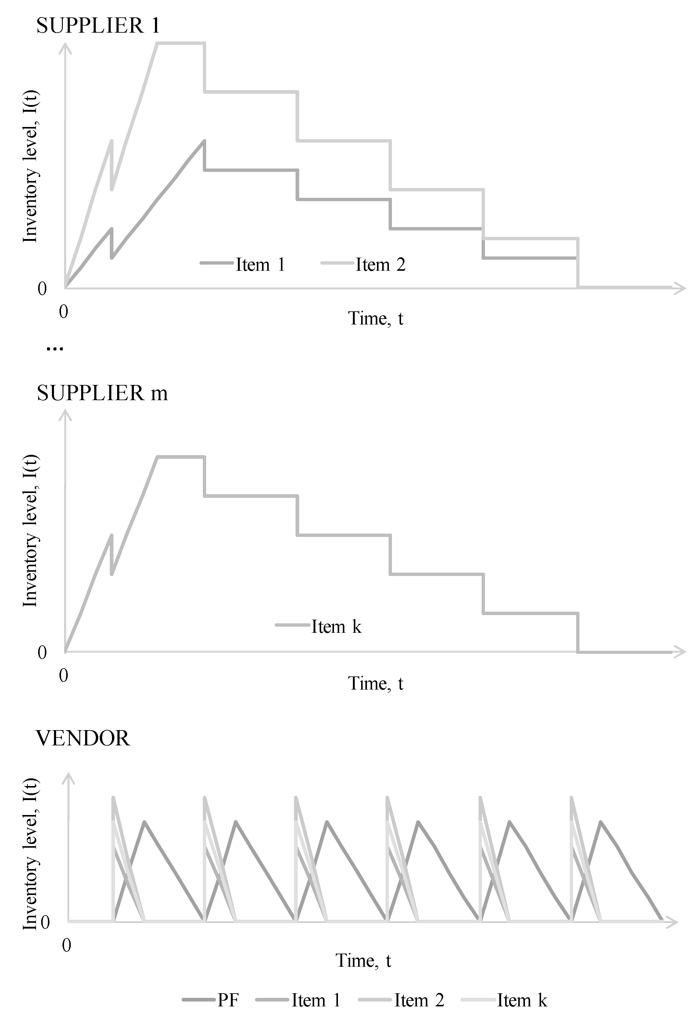
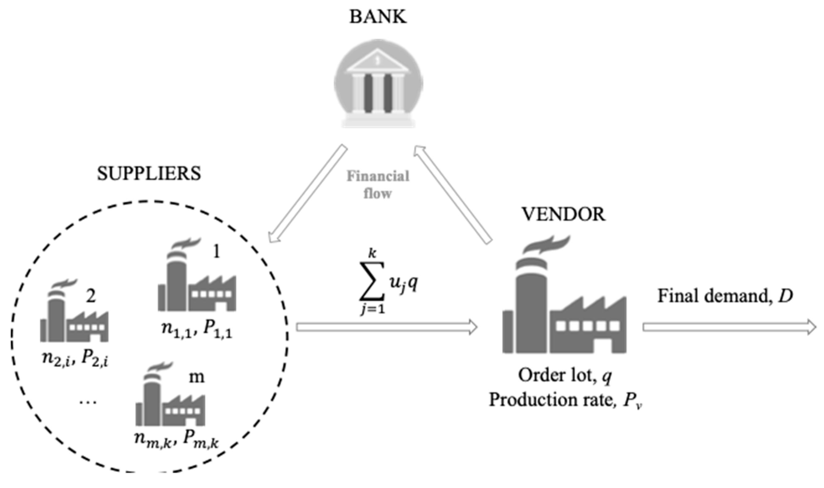
This paper deals with the coordination of inventory and financing decisions in a two-level supply chain with multi-suppliers and a vendor. Replenishments follow an equal-sized shipment policy. Hence, the vendor orders a lot size of u j q for every part j at regular time intervals and starts its production process at a rate of P v manufacturing lot of size q . The suppliers manufacture lots of size n s , j u j q at a finite production rate P s , j with a single setup that is delivered to the vendor in n s , j shipments of equal size u j q . The suppliers incur a setup cost for each production run, while the vendor incurs an ordering cost for each order placed. A vendor may receive one or more (product) parts from a supplier to assemble the product that it sells to costumers. Figure 3 shows the behavior of inventory overtime for the suppliers and the vendor for different produced and shipped parts. The vendor, whose role is central to the supply chain, adopts a reverse factoring agreement through a financial institution (e.g., a bank) to manage its accounts payables with its suppliers at the least possible cost. Figure 4 is a schematic representation of the supply chain consisting of multi-suppliers and a vendor, with a bank (third party) managing the financial flows.
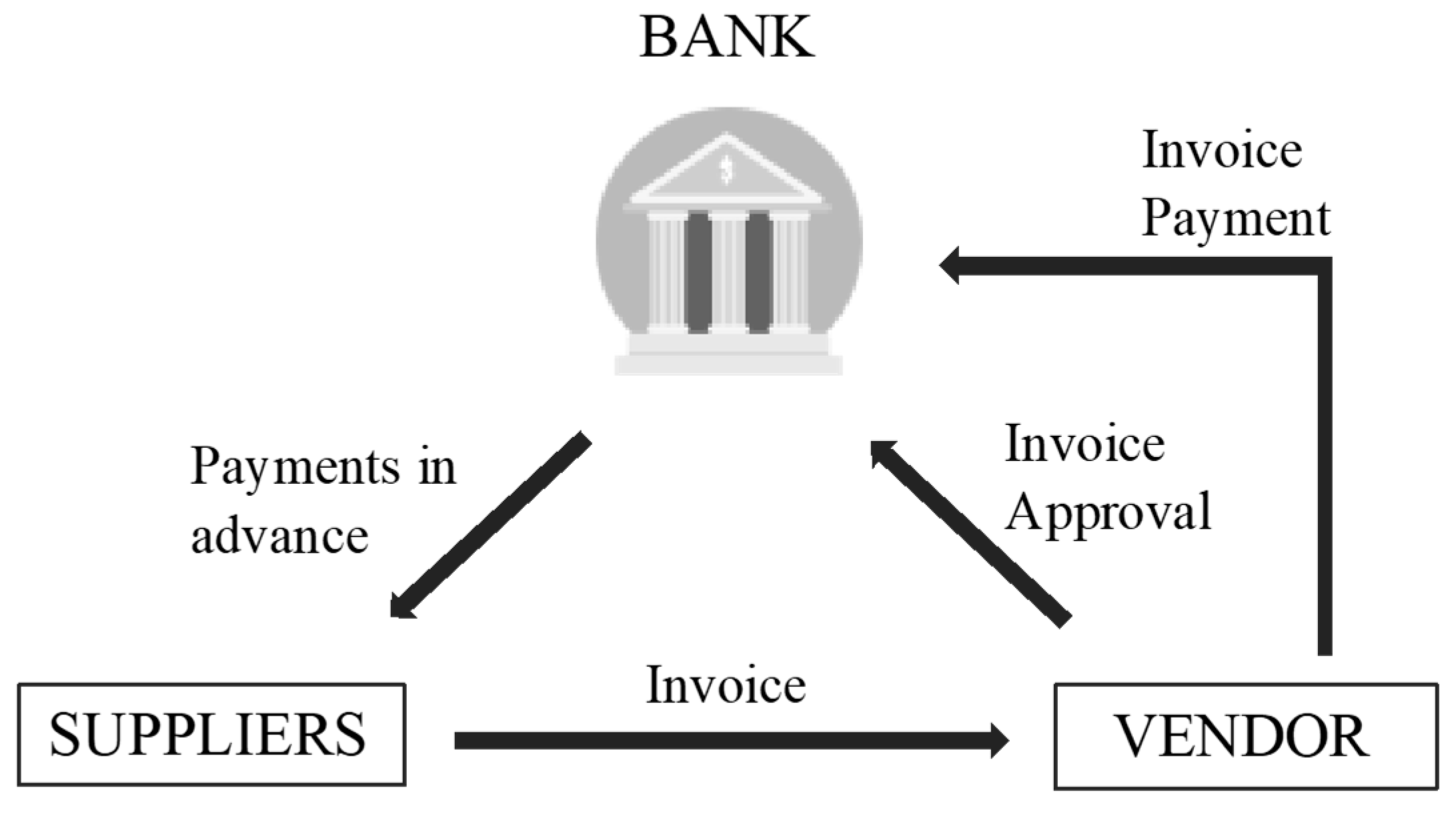
Reverse Factoring (RF), specifically, is a financial solution where the vendor (who is ordering) contacts its bank to arrange for early payments to its supplier to finance their accounts receivables (from purchases) at interest rates lower than the market (Van Der Vliet et al. 2015). The vendor is assumed to have a better financial position (liquidity and solvency) than its suppliers. Once the vendor receives invoices of orders, it immediately notifies its bank to make payments to its suppliers without delay or by the due date specified in the trade agreement. At the same time, the bank provides an approved-invoice-based financing solution to the suppliers through early payments, as shown in Figure 5. This arrangement furnishes the necessary capital for its suppliers to start production with minimal financial risks since mostly they are carried by the vendor (Lekkakos and Serrano 2016). RF reduces the unit cost of borrowing for the suppliers since the vendor leverages the cost of capital (Lekkakos and Serrano 2017).
The following straightforward JELS assumptions are made in addition to the properties already described (Jaber and Goyal 2008):
  • Deterministic demand and constant over time which is lower than the production rate of the vendor P v ;
  • The final product requires k different parts;
  • Shortages are not allowed;
  • Lead time is assumed to be zero;
  • An infinite time horizon is considered.
The JELS with reverse factoring is developed in Section 3.2. A reference case model, JELS without reverse factoring, is presented in Section 3.3. The two models are then compared.

3.2. Model Development

3.2.1. The Vendor’s Annual Profit Function

The vendor’s annual revenue from selling the final product to the end customer is p v D . Its annual cost components are explained next. The ordering cost of parts (components) from its suppliers is ( A v + j = 1 k a v , j ) D / q . The purchasing cost of raw materials and components required to produce the final product is s = 1 m j = 1 k u j p s , j D Y s , j . The production setup cost is S D / q . The transforming cost of purchased components of a unit of the final product is c 0 D . The costs of stocking raw materials and components at the vendor’s warehouse are j = 1 k h v , j u j q D / 2 P v and h v , P F ( 1 D / P v ) q / 2 , respectively. Furthermore, due to the establishment of the reverse factoring agreement, the vendor pays interests to the bank for each unit of raw material and component paid in advance by the financial institution to the suppliers. The interest rate of the vendor ( ρ v ) is applied to the value of the purchased parts in each production cycle, p s , j u j q , multiplied by the advance period, i = 1 n s , j [ u j q / P s , j + ( i 1 ) q / D ] . The total annual profit of the vendor, T P V , is thus the sum of the revenues minus the costs as defined in Equation (1).
T P V ( q ) = p v D c 0 D s = 1 m j = 1 k u j p s , j D Y s , j ( S + A v + j = 1 k a v , j ) D q j = 1 k h v , j u j q D 2 P v h v , P F q 2 ( 1 D P v ) s = 1 m j = 1 k i = 1 n s , j p j D n s , j ρ v [ u j q P s , j + ( i 1 ) q D ] Y s , j
where h v consists of two components, physical, h v , p , and a financial h v , f . The financial holding component is linked to the value of the material stored and to the vendor’s capital cost and is determined as h v , P F , f = ρ v ( c 0 + s = 1 m j = 1 k p s , j u j Y s , j ) , while h v , j , f = ρ v p s , j .

3.2.2. The Suppliers’ Annual Profit Function

The total annual profit of each supplier, T P S , s , is given by the sum of the revenues from selling the parts to the vendor which are paid in advance from the bank ( j = 1 k p s , j u j D ), minus the production costs ( j = 1 k c s , j u j D ), the costs for the setups required to produce the k s parts ( j = 1 k A s , j D / n s , j q ), and the holding costs to stock the parts’ inventories in the warehouse ( j = 1 k h s , j u j q [ ( 1 u j D / P s , j ) n s , j + 2 u j D / P s , j 1 ] / 2 ). The formulation of T P S , s for a generic supplier s is given as:
T P S , s ( n s , j ) = j = 1 k { ( p s , j c s , j ) u j D A s , j D n s , j q h s , j u j q 2 [ ( 1 u j D P s , j ) n s , j + 2 u j D P s , j 1 ] } Y s , j
where h s , j consists of two components, physical, h s , j , p , and financial h s , j , f . The financial holding cost is the production cost of unit j manufactured by supplier s, c s , j , multiplied by the discounted interest rate that the supplier receives when reverse factoring, ρ s , in applied and it is h s , j , f = c s , j ρ s .

3.2.3. The Supply Chain’s Annual Profit Function

The supply chain total profit function is determined by adding the profit of the vendor to the ones of the multiple suppliers as:
T P S C ( n s , j , q ) = T P V + s = 1 m T P S , s
T P S C ( n s , j , q ) = ( p v c 0 s = 1 m j = 1 k c s , j u j Y s , j ) D ( S + A v + j = 1 k a v , j + s = 1 m j = 1 k A s , j n s , j Y s , j ) D q j = 1 k h v , j u j q D 2 P v h v , P F q 2 ( 1 D P v ) s = 1 m j = 1 k h s , j u j q 2 [ ( 1 u j D P s , j ) n s , j + 2 u j D P s , j 1 ] Y s , j s = 1 m j = 1 k i = 1 n s , j p j D n s , j ρ v [ u j q P s , j + ( i 1 ) q D ] Y s , j

3.2.4. Solution Procedure

This section presents a solution procedure to find the optimal values of the decision variables. We start by finding the first and second partial derivatives of Equation (4) with respect to q. As can be seen from Equation (6), the total supply chain profit function is concave in q for given values of n s , j ≥ 1. A closed-form solution for q is then determined by setting the first partial derivative of Equation (5) equal to zero and solving for q to get Equation (7).
T P S C q = ( S + A v + j = 1 k a v , j + s = 1 m j = 1 k A s , j n s , j Y s , j ) D q 2 j = 1 k h v , j u j D 2 P v h v , P F 2 ( 1 D P v ) s = 1 m j = 1 k h s , j u j 2 [ ( 1 u j D P s , j ) n s , j + 2 u j D P s , j 1 ] Y s , j s = 1 m j = 1 k i = 1 n s , j p j D n s , j ρ v [ u j q P s , j + ( i 1 ) q D ] Y s , j
2 T P S C q 2 = 2 ( S + A v + j = 1 k a v , j + s = 1 m j = 1 k A s , j n s , j Y s , j ) D q 3 < 0
q * = N 0 N 1 + N 2 + N 3
where
  • N 0 = 2 ( S + A v + j = 1 k a v , j + s = 1 m j = 1 k A s , j n s , j Y s , j ) D
  • N 1 = j = 1 k h v , j u j D P v + h v , P F ( 1 D P v )
  • N 2 = h v , P F ( 1 D P v ) + s = 1 m j = 1 k h s , j u j [ ( 1 u j D P s , j ) n s , j + 2 u j D P s , j 1 ] Y s , j
  • N 3 = 2 s = 1 m j = 1 k i = 1 n s , j p j D n s , j ρ v [ u j P s , j + ( i 1 ) 1 D ] Y s , j
The optimal values of the number of supplier’s shipments for every part are determined by following the steps below. The optimal values of the number of shipments, n s , j   s   ϵ   [ 1 , m ] and   j   ϵ   [ 1 , k ] , are complex to be analytically obtained in a closed-form expression. Therefore, these values were numerically determined using Excel Solver enhanced with Visual Basic for Applications (VBA) code, with nested search loops (Jaber and Goyal 2008). However, the tool is limited, as it does not guarantee a globally optimal solution.

3.3. Reference Case without Reverse Factoring

To evaluate the trade-off between costs and benefits of introducing a reverse factoring, the model developed in this paper is compared to a reference model (case) with no financial schemes. The total profit of the vendor for the reference case is given as:
T P V , 0 ( q ) = ( p v c 0 s = 1 m j = 1 k u j p s , j Y s , j ) D ( S + A v + j = 1 k a v , j ) D q j = 1 k h v , j u j q D 2 P v h v , P F q 2 ( 1 D P v )
Moreover, since without a reverse factoring agreement, the suppliers have higher financial risks, they face a higher capital cost, and, consequently, a higher holding cost ( h s , j , f , 0 = c s , j ρ s , j , 0 ). The annual total profit of the suppliers is, therefore, given as:
T P S , s , 0 ( n s , j ) = j = 1 k { ( p s , j c s , j ) u j D A s , j D n s , j q h s , j , 0 u j q 2 [ ( 1 u j D P s , j ) n s , j + 2 u j D P s , j 1 ] } Y s , j
Evaluating the first and second partial derivatives of the annual total profit of the supply chain ( T P S C , 0 = T P V , 0 + s = 1 m T P S , s , 0 ) in q it is possible to detect that a closed-formulation for the optimal order lot size can be obtained. Then, setting the first derivative equal to zero, where the optimal lot size quantity is given as:
q * = 2 ( S + A v + j = 1 k a v , j + s = 1 m j = 1 k A s , j n s , j Y s , j ) D j = 1 k h v , j u j D P v + h v , P F ( 1 D P v ) + s = 1 m j = 1 k h s , j , 0 u j [ ( 1 u j D P s , j ) n s , j + 2 u j D P s , j 1 ] Y s , j
The optimal values of the supplier’s number of shipments for every part are determined using the same solution algorithm proposed in the previous subsection.

4. Numerical Example

This section presents a numerical study to illustrate the behavior of the model presented above. The parameters used for the modeling of the vendor process were adapted from the literature (Jaber and Goyal 2008) and are listed below: A v = 100 $/order, c 0 = 15 $/unit, D = 1000 unit/year, h v , p = 2 $/unit⋅year, p v = 200 $/unit, ρ v = 1 % , and S = 200 $/setup. The vendor purchases three types of materials/components from two suppliers to produce one unit of the final product. Table 1 lists the input data on the suppliers and the related components.
The model with reverse factoring presented, in Section 3.2, i.e., Equations (1)–(4) and (7), is solved using the procedure described in Section 3.2.4. The reference model, without the reverse factoring agreement, i.e., Equations (8)–(10), is also solved for the above data using the solution procedure described earlier.
The results of the numerical example are reported in Table 2. The results show that for the input parameters in Table 1, with reverse factoring, the supply chain total annual profit, TPSC, increases by 3.23% (from 57,313 to 59,161) and the lot size quantity by 8.4% (from 202 to 219).
The results in Table 2 show that not all players benefit from reverse factoring. The vendor’s profit reduces by 1.38% (from 17,849 to 17,602), while those of Suppliers 1 and 2, respectively, increase by 4.6% (from 31,015 to 32,438) and 7.93% (from 8450 to 9120). Although the vendor is the one who pays off the interest charges to the financial institution resulting in lower total profit, it should be noted that it achieves additional intangible economic and operational benefits from managing its supply chain and its relationship with the bank. For example, reverse factoring helps the vendor in reducing the complexity of purchase and payment transactions and the default risk associated with strategic partners. It also allows the vendor to build long-term and transparent relationships with its suppliers based on trust and collaboration and in enabling an economically sustainable supply chain. Supplier 2, which furnishes the third part, experiences a significant increase in its total annual profit, compared to Supplier 1. This increase has to do with the high purchase cost of the third component and to the supplier’s weak financial position (i.e., a high cost of capital, ρ s , 0 ), significantly increasing the financial holding cost and, consequently, a better chance of making a reverse factoring agreement work. The results in Table 2 show that the production lot sizes for the suppliers increase with reverse factoring. For example, lot sizes for parts 1 and 2 furnished by the first supplier, n 1 , 1 q and n 1 , 2 q , increases by 36% (from 807 to 1093) and 63% (from 403 to 656), respectively. The lot size for part 3 furnished by Supplier 2, n 2 , 3 q , increases by 63% (from 403 to 656). These results have to do with the suppliers receiving a lower interest rate, thus reducing their financial holding cost, which allows them to carry more inventory.
The relatively limited increase in the total profit due to the introduction of the reverse factoring agreement is due to the high share of non-differential cost components (i.e., revenues, production, and purchasing costs). Hence, hereafter, it presents an analysis with a focus on the only differential costs. Table 3 shows that the vendor is subject to an 11.5% increase in the differential costs due to the high impact of the interest charged by the bank. On the contrary, suppliers face a significant decrease in differential costs (i.e., −35.8% and −43.2% for Supplier 1 and Supplier 2, respectively). The supply chain on the overall is subject to a 24.05% reduction of these costs.
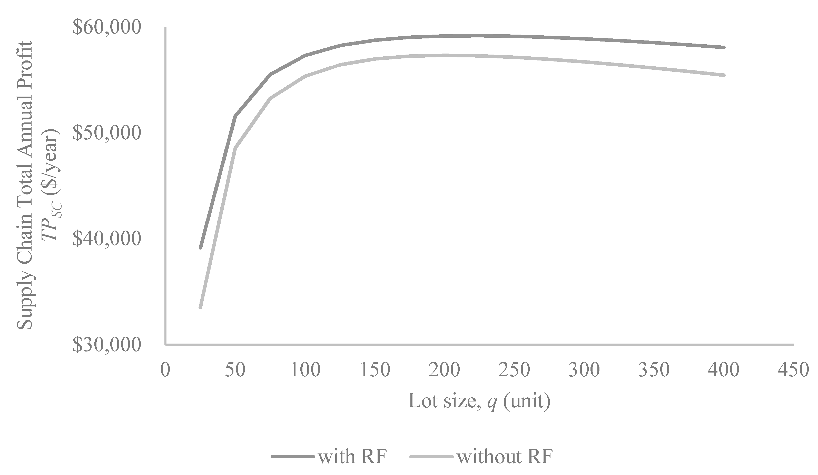
Figure 6 shows the behavior of the supply chain total annual profits, T P S C ( n s , j , q ) , from Equation (4), and T P S C , 0 , from Equations (8) and (9), with and without a reverse factoring agreement, respectively, for different values of q . The profit functions show, as in Equation (6), a concave behavior in q . The results in Figure 6 show that the supply chain has higher profits for a wide range of q when reverse factoring is adopted. They show that since the total annual profit of the supply chain is concave in q , an optimal value of the lot size q exists. Interestingly, T P S C ( n s , j , q ) is less sensitive to q than T P S C , 0 is. For example, between q = 175 and q = 400, Δ T P S C ( n s , j , q ) = |58,063.78−59,015.96| = 952.18 and Δ T P S C , 0 = |55,437.95−57,235.69| = 1797.74, or Δ T P S C ( n s , j , q ) / Δ q = 4.23 and Δ T P S C , 0 / Δ q = 7.99, respectively. With reverse factoring, the supply chain has more flexibility in setting its order quantity. That is, for any reason, if the vendor has to order off its optimum quantity, for instance to q = 175, then the cost of doing so, Δ T P S C ( n s , j , q ) , is about 53% of Δ T P S C , 0 , which represents the cost when reverse factoring is not considered. This differential cost is easy to absorb by the supply chain, and the players can easily find ways to do that. However, it becomes more difficult to absorb and encounter when the cost is significantly high.
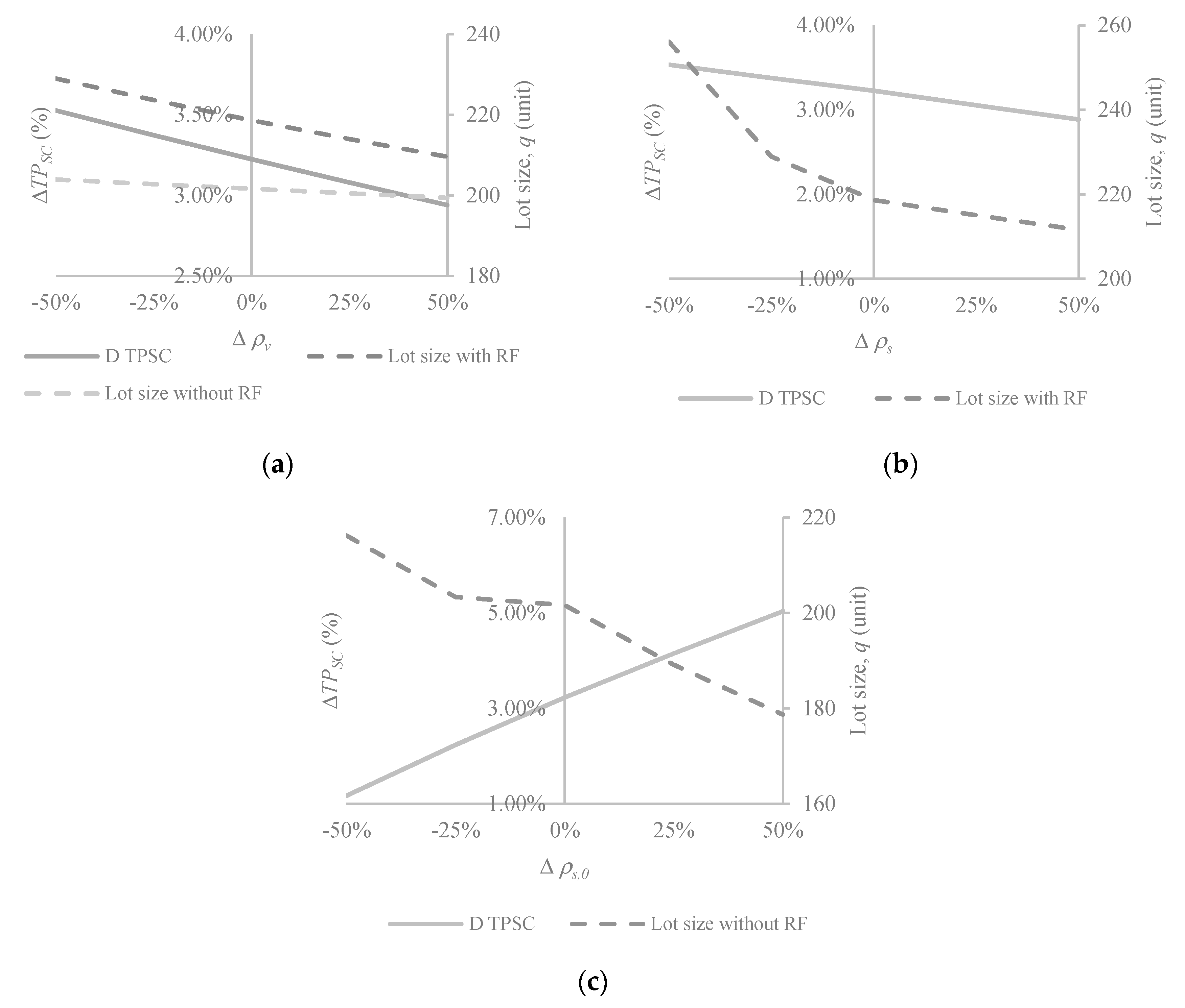
The interest rates of the vendor and the suppliers are the relevant parameters of this study. Figure 7 shows the sensitivity of the supply chain profit and the lot size quantity for changes in the values of the interest rates. The input parameters in Table 1 were used to produce the results in Figure 7. The interest rates were varied one at a time. The figure has three parts (a, b, and c) that plot changes in the supply chain total annual profit, Δ T P S C , and the corresponding lot sizes with and without reverse factoring against the percentage variation in the interest rates of the vendor and the suppliers with and without reverse factoring, Δ ρ v , Δ ρ s , and Δ ρ s , 0 . Figure 7a shows that increasing Δ ρ v reduces Δ T P S C , making a reverse factoring agreement less appealing as the interest gap between the vendor and the supplier is narrow. An increase in ρ v reduces the lot size, q, for both the scenario, but with a higher impact on the case with reverse factoring. Δ T P S C in Figure 7b shows similar behavior to that in Figure 7a when Δ ρ s is varied instead of Δ ρ v . The lot size with RF, however, shows a non-linear decrease rather than linear due to variations of the optimal number of shipments. Figure 7c shows that Δ T P S C and q have opposite behavior for changes in Δ ρ s , 0 (without reverse factoring), where increasing ρ s , 0 increases Δ T P S C and reduces q .

5. Summary and Conclusions

This paper proposed a joint economic lot size model in which a vendor coordinates operational and financial decisions with several suppliers through a reverse factoring arrangement with a bank as a third player. In particular, the vendor systematically informs a financial institution (e.g., a bank) of its payment obligations to its suppliers. In this way, the latter can access cheaper interest rates. Numerous numerical results were generated to illustrate the behavior of the developed model. The results showed that the establishment of a reverse factoring agreement between the players in the supply chain increases the supply chain’s total annual profit and affects the operational decisions (i.e., optimum lot size and the number of shipments for each component).
A reverse factoring agreement has the potential of success and to bring additional benefits to a supply chain, especially when financially weak suppliers face increases in demand. Start-ups are a reality of modern markets. They, for instance, could be suppliers for vendors in supply chains that struggle initially because of slow demand, which could be due to limited production capacity that usually grows with time and experience (learning). Such companies have weak financial positions and critical economic performance that restrict them from accessing cash at low rates as banks consider them risky investments. A possible extension of this study is to consider the maximization of the annuity stream instead of the total annual profit, which helps in identifying the revenues and costs arising from time shifts between payments. Other future research may deal with different supply chain settings affecting the financial flow of the companies (Ramezani et al. 2014). For instance, it could be interesting to assess the effect of the reverse factoring agreement in reverse-flow and closed-loop supply chains.

Author Contributions

The authors worked collectively on the manuscript preparation, modification, and review. All authors have read and agreed to the published version of the manuscript.

Funding

M.Y. Jaber thanks the Natural Sciences and Engineering Research Council of Canada (NSERC) for supporting his research, and the Università degli Studi di Brescia for the in-kind support.

Conflicts of Interest

The authors declare no conflict of interest.

References

  1. Aljazzar, Salem M., Mohamad Y. Jaber, and Lama Moussawi-Haidar. 2017. Coordination of a three-level supply chain (supplier-manufacturer-retailer) with permissible delay in payments and price discounts. Applied Mathematical Modelling 48: 289–302. [Google Scholar] [CrossRef]
  2. Aljazzar, Salem M., Amulya Gurtu, and Mohamad Y. Jaber. 2018. Delay-in-payments—A strategy to reduce carbon emissions from supply chains. Journal of Cleaner Production 170: 636–44. [Google Scholar] [CrossRef]
  3. Banerjee, Avijit. 1986. A Joint Economic-Lot-Size Model for Purchaser and Vendor. Decision Sciences 17: 292–311. [Google Scholar] [CrossRef]
  4. Caniato, Federico, Luca M. Gelsomino, Alessandro Perego, and Stefano Ronchi. 2016. Does finance solve the supply chain financing problem? Supply Chain Management 21: 534–49. [Google Scholar] [CrossRef]
  5. Dello Iacono, Umberto, Matthew Reindorp, and Nico Dellaert. 2015. Market adoption of reverse factoring. International Journal of Physical Distribution & Logistics Management 45: 286–308. [Google Scholar] [CrossRef]
  6. Gelsomino, Luca M., Riccardo Mangiaracina, Alessandro Perego, and Angela Tumino. 2016. Supply chain finance: A literature review. International Journal of Physical Distribution & Logistics Management 46: 348–66. [Google Scholar] [CrossRef]
  7. Glock, Christoph H. 2011. A multiple-vendor single-buyer integrated inventory model with a variable number of vendors. Computers & Industrial Engineering 60: 173–82. [Google Scholar] [CrossRef]
  8. Glock, Christoph H. 2012. The joint economic lot size problem: A review. International Journal of Production Economics 135: 671–86. [Google Scholar] [CrossRef]
  9. Glock, Christoph H., and Taebok Kim. 2014. Shipment consolidation in a multiple-vendor-single-buyer integrated inventory model. Computers & Industrial Engineering 70: 31–42. [Google Scholar] [CrossRef]
  10. Goyal, Suresh K. 1977. An integrated inventory model for a single supplier-single customer problem. International Journal of Production Research 15: 107–11. [Google Scholar] [CrossRef]
  11. Hofmann, Erik. 2005. Supply Chain Finance: Some conceptual insights. Logistik Management: Innovative Logistikkonzepte 80: 203–14. [Google Scholar] [CrossRef]
  12. Hurtrez, Nicolas, and Massimo G. S. Salvadori. 2010. Supply chain finance: From myth to reality. In McKinsey on Payments. pp. 22–28. Available online: https://www.finyear.com/attachment/252360 (accessed on 7 April 2020).
  13. Jaber, Mohamad Y., and Suresh K. Goyal. 2008. Coordinating a three-level supply chain with multiple suppliers, a vendor and multiple buyers. International Journal of Production Economics 116: 95–103. [Google Scholar] [CrossRef]
  14. Kim, Taebok, and Suresh K. Goyal. 2009. A consolidated delivery policy of multiple suppliers for a single buyer. International Journal of Procurement Management 2: 267. [Google Scholar] [CrossRef]
  15. Klapper, Leora. 2006. The role of factoring for financing small and medium enterprises. Journal of Banking and Finance 30: 3111–30. [Google Scholar] [CrossRef] [Green Version]
  16. Kraemer-Eis, Helmut, Antonia Bostari, Salome Gvetadze, Frank Lang, and Wouter Torfs. 2018. European Small Business Finance Outlook. Luxembourg: European Investment Fund. [Google Scholar]
  17. Lekkakos, Spyridon D., and Alejandro Serrano. 2016. Supply chain finance for small and medium sized enterprises: The case of reverse factoring. International Journal of Physical Distribution & Logistics Management 46: 367–92. [Google Scholar] [CrossRef]
  18. Lekkakos, Spyridon D., and Alejandro Serrano. 2017. Reverse factoring: A theory on the value of payment terms extension. Foundations and Trends in Technology, Information and Operations Management 10: 270–88. [Google Scholar] [CrossRef] [Green Version]
  19. Marchi, Beatrice, Jörg M. Ries, Simone Zanoni, and Christoph H. Glock. 2016. A joint economic lot size model with financial collaboration and uncertain investment opportunity. International Journal of Production Economics 176: 170–82. [Google Scholar] [CrossRef]
  20. Marchi, Beatrice, Simone Zanoni, Ivan Ferretti, and Lucio E. Zavanella. 2018. Stimulating Investments in Energy Efficiency through Supply Chain Integration. Energies 11: 858. [Google Scholar] [CrossRef] [Green Version]
  21. Marchi, Beatrice, Lucio E. Zavanella, and Simone Zanoni. 2020. Joint economic lot size models with warehouse financing and financial contracts for hedging stocks under different coordination policies. Journal of Business Economics. [Google Scholar] [CrossRef]
  22. Modigliani, Franco, and Merton H. Miller. 1958. The cost of capital, corporation finance, and the theory of investment. The American Economic Review 48: 261–97. [Google Scholar]
  23. Observatory for Supply Chain Finance. 2016. Supply Chain Finance: Opportunities in the Italian Market. Milano: Politecnico di Milano. [Google Scholar]
  24. Observatory for Supply Chain Finance. 2017. Supply Chain Finance: Tomorrow Is Already Here! Milano: Politecnico di Milano. [Google Scholar]
  25. Ouyang, Liang-Yuh, Chia-Huei Ho, and Chia-Hsien Su. 2009. An optimization approach for joint pricing and ordering problem in an integrated inventory system with order-size dependent trade credit. Computers & Industrial Engineering 57: 920–30. [Google Scholar] [CrossRef]
  26. Pfohl, Hans-Christian, and Moritz Gomm. 2009. Supply chain finance: Optimizing financial flows in supply chains. Journal of Logistics Research 1: 149–61. [Google Scholar] [CrossRef]
  27. Ramezani, Majid, Ali M. Kimiagari, and Behrooz Karimi. 2014. Closed-loop supply chain network design: A financial approach. Applied Mathematical Modelling 38: 4099–119. [Google Scholar] [CrossRef]
  28. Randall, Wesley S., and Martin Theodore II Farris. 2009. Supply chain financing: Using cash-to-cash variables to strengthen the supply chain. International Journal of Physical Distribution & Logistics Management 39: 669–89. [Google Scholar] [CrossRef]
  29. Tanrisever, Fehmi, Hande Cetinay, Matthew Reindorp, and Jan C. Fransoo. 2015. Reverse Factoring for SME Finance. SSRN. [Google Scholar] [CrossRef]
  30. Van Der Vliet, Kasper, Matthew J. Reindorp, and Jan C. Fransoo. 2015. The price of reverse factoring: Financing rates vs. payment delays. European Journal of Operational Research. [Google Scholar] [CrossRef] [Green Version]
  31. Wagner, Stephan M. 2006. A firm’s responses to deficient suppliers and competitive advantage. Journal of Business Research 59: 686–95. [Google Scholar] [CrossRef]
  32. Wu, Yaobin, Yingying Wang, Xun Xu, and Xiangfend Chen. 2019. Collect payment early, late, or through a third party’s reverse factoring in a supply chain. International Journal of Production Economics 218: 245–59. [Google Scholar] [CrossRef]
  33. Wuttke, David A., Constantin Blome, and Michael Henke. 2013. Focusing the financial flow of supply chains: An empirical investigation of financial supply chain management. International Journal of Production Economics 145: 773–89. [Google Scholar] [CrossRef]
  34. Wuttke, David A., Constantin Blome, Sebastian Heese, and Margarita Protopappa-Sieke. 2016. Supply chain finance: Optimal introduction and adoption decisions. International Journal of Production Economics 178: 72–81. [Google Scholar] [CrossRef]
  35. Xu, Xinhan, Xiangfeng Chen, Fu Jia, Steve Brown, Yu Gong, and Yifan Xu. 2018. Supply chain finance: A systematic literature review and bibliometric analysis. International Journal of Production Economics 204: 160–73. [Google Scholar] [CrossRef]
  36. Zhan, Jizhou, Shuting Li, and Xiangfeng Chen. 2018. The impact of financing mechanism on supply chain sustainability and efficiency. Journal of Cleaner Production 205: 407–18. [Google Scholar] [CrossRef]
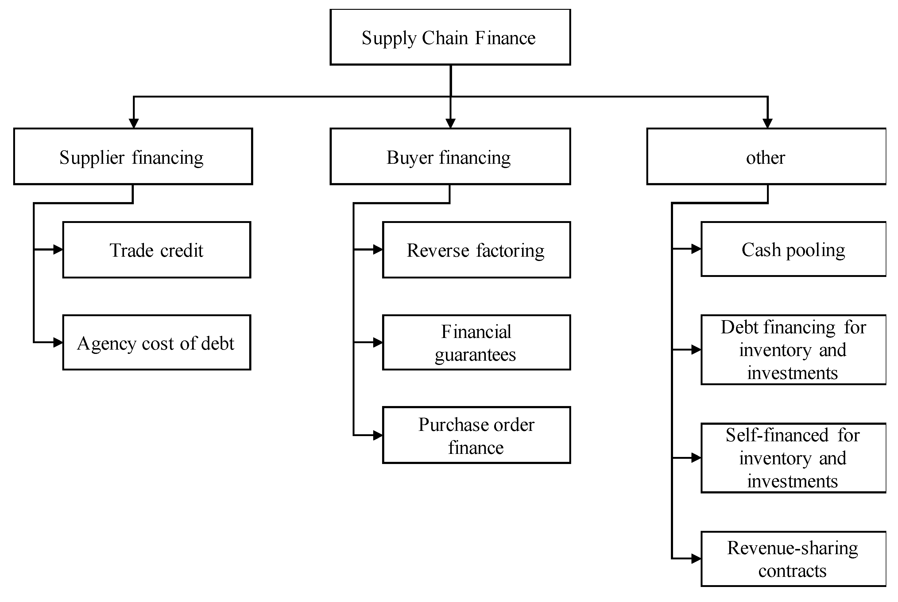
Figure 1. Supply chain finance solutions.
Ijfs 08 00023 g001
Figure 2. Classification of the main supply finance solutions (Observatory for Supply Chain Finance 2016).
Ijfs 08 00023 g002
Figure 3. The inventory behavior for the suppliers and the vendor.
Ijfs 08 00023 g003
Figure 4. Schematic representation of a supply chain consisting of multi-suppliers, a vendor, and a bank (third party), who manages the financial flows.
Ijfs 08 00023 g004
Figure 5. Schematic representation of the reverse factoring mechanism.
Ijfs 08 00023 g005
Figure 6. Supply chain total annual profit as a function of the lot size for the cases with and without a reverse factoring agreement.
Ijfs 08 00023 g006
Figure 7. Optimal lot size, and total cost of the supply chain as a function of interest rates: (a) of the vendor ρ v , (b) of the supplier with reverse factoring ρ s , and (c) of the supplier without reverse factoring ρ s , 0 .
Ijfs 08 00023 g007
Table 1. Input data.
SupplierPartUnits for One Part of Final Product ( u j )Order Cost ( a v , j )Setup Cost ( A s , j )Unit Production Cost ( c s , j )Production Rate ( P s , j )Selling Price ( p s , j )Physical Holding Cost ( h s , j , p ) ρ s ρ s , 0
115104001055001512%15%
12210400203500252
23153003015004023%20%
Table 2. Results of the numerical example.
Caseqn1,1n1,2n2,3TPVTPS,1TPS,2TPSC Δ T P S C
with RF219533$17,602$32,438$9120$59,161+3.23%
without RF202422$17,849$31,015$8450$57,313
Table 3. Analysis of the differential costs with and without a reverse factoring agreement.
VendorSupplier 1Supplier 2
CaseSETUP COSTOrder CostHolding CostInterest to the BankSetup CostHolding CostSetup CostHolding Cost
with RF$915$572$585$327$976$1585$457$423
without RF$992$620$539-$1488$2498$744$807