The Impact of Macroeconomic News on Chinese Futures

Abstract

Inspired by the GARCH-MIDAS model, we revisit the relationship between Chinese futures and macroeconomic factors. We introduce the level of the macroeconomic variables into the GARCH-MIDAS model in order to test the impact of the macroeconomic level on the variance of futures’ return volatility. Based on the empirical results, we find the level of macroeconomic variables has a significant impact on the volatility of Chinese futures’ return. The influence of the macroeconomic level factor on the futures’ return volatility is statistically significant.

1. Introduction

There is extensive literature that the emerging and developed futures market returns are sensitive to macroeconomic news. Futures market participants tend to follow closely the release of economic data and announcements of macroeconomic change. How do macroeconomic fundamentals influence Chinese futures’ market returns? Is the impact statistically significant? This research attempts to answer these questions by investigating the link between the macroeconomic variables and the stock return volatility in the Chinese futures market.

Chinese futures have revealed remarkable price volatility in recent decades. The Chinese futures market entered a remarkable fluctuation in 2008, with the advent of the Financial Samurai. The fluctuation of a futures price influences investors’ decisions. Producers and consumers of the commodity pay more to cover the uncertainty in the commodity futures market. Understanding the relation between macroeconomic fundamentals and Chinese futures market returns is valid for the investors who want to hedge against the risk and optimize the portfolio.

As an emerging market, the Chinese futures market has begun to play a significant role in the world financial derivatives market. In 1990, the first Chinese commodity futures exchange was established in Zhenzhou. There are four futures exchanges in China, the Zhengzhou Commodity Exchange (ZCE, established in 1993), Dalian Commodity Exchange (DCE, established in February 1993), Shanghai Futures Exchange (SHFE, established in 1999), and China Financial Futures Exchange (CFFEX, established in Shanghai in September 2006). In 2007, the trading volumes of ZCE, DCE, and SHFE reached 586, 1019 and 1364 million, respectively (data from World Federation of Exchange).

This paper reveals the relationship between the macroeconomic fundamentals and futures prices volatility in China’s futures market. Three essential questions are addressed in the paper. First, what is the impact of macroeconomic variables on the volatility of futures’ prices? Second, does the macroeconomic variables impact the commodities futures and the index futures in the same way? Third, how to measure the impact of the macroeconomic variables?

The answers to these questions are important for several reasons: first, in the research, the futures return data is daily data, while the macroeconomic data is monthly data. This research can explore the daily futures market reaction to monthly macroeconomic data. This research provides empirical evidence that illustrates the link between low-frequency macroeconomic news and high-frequency futures price volatility. Second, compared with research on the commodity futures market, this research investigates how the stock index futures respond to the macroeconomic news. As an essential financial derivative, stock index futures contracts are widely traded in China’s financial futures exchanges. The fluctuation of the futures prices significantly affect the investors in the stock market and futures market. Last, the study provides comprehensive research on China’s futures market.

The previous study reveals the influence of macroeconomic fundamentals on the commodity market and stock market. Ghosh et al. (2004), Gorton and Rouwenhorst (2006), and Mahdavi and Zhou (1997) test the relationship between inflation and the commodity market, and they employ the consumer price index (CPI) as the macroeconomic variable. Batten et al. (2010), Karali and Power (2013), Karali and Ramirez (2014) employ industrial production (IP) as the macroeconomic determinant of the commodity market. Prokopczuk and Symeonidis (2013), Frankel (2014), Dönmez and Magrini (2013) test the impact of monetary policy on the commodities market. They choose the money supply and the short-term interest rate as the monetary variable. Arouri et al. (2011); Malik and Ewing (2009); Malik and Hammoudeh (2007); and Thuraisamy et al. (2013) test the stock market influence on the commodity market. In the research, they employ the stock index as the macroeconomic variable.

In this research, we employ the GARCH-MIDAS model proposed by Engle et al. (2013) to test the relation between the China futures market volatility and macroeconomic news. This model combines the GARCH model proposed by Engle and Lee (1999), and Engle and Rangel (2008) and the MIDAS framework of Ghysels et al. (2006). The GARCH-MIDAS model solves the data mismatching frequency of daily returns and monthly or quarterly macroeconomic variables. This model employs the mean-reverting daily GARCH process and the use of the MIDAS approach. The GARCH-MIDAS model decomposes the conditional variance into the short-run and long-run variance, the short-run variance is decided by the mean-reverting GARCH (1,1) process, the secular component of the variance is determined by the history of the realized variance, or macroeconomic variables weighted MIDAS polynomials.

The GARCH-MIDAS model is widely used in research of the financial markets. Asgharian et al. (2013) and Conrad and Loch (2015) use the GARCH-MIDAS model to explore the relationship between the macroeconomic fundamentals and U.S. stock market volatility. Mo et al. (2018), Fang et al. (2018), and Asgharian et al. (2013) use the GARCH-MIDAS model to explore the impact of macroeconomic fundamentals on the emerging commodities futures market.

The finding of this research contributes to the existing literature, which tests the relation between the macroeconomic variables and the financial derivatives market. Thorough research is undertaken into Chinese futures contracts, including the commodity futures and stock index futures. The research gives the market participants and the policymakers references. The investor can make the reinvestment decision according to macroeconomic changes. The policymakers can adjust macroeconomic policies to achieve financial stability.

The finding of the research is as follows: in China commodity market, the inflation indexes such as CPI and producer price index (PPI) have a positive impact on the commodity futures returns’ volatility. Which means the increase of CPI and PPI index will increase the volatility in the commodity. Industrial production, money supply (M2), and the interest rate have an opposite effect on the commodity futures market. For the CSI 300 futures market, the levels of the macroeconomic variables have a negative influence on the stock index futures returns’ volatility. This means high-level CPI, PPI, IP, and M2 will decrease the volatility in the stock index futures market. Based on the parameter estimates, the macroeconomic impacts are statistically significant.

The remainder of the paper is organized as follows: Section 2 is data and methodology. The data refers to the Chinese commodities futures market and the macroeconomic variables. The methodology describes the GARCH-MIDAS model. Section 3 covers the empirical implement. The last part is the conclusion of the paper.

2. Data and Methodology

To undertake comprehensive research on the Chinese futures market, we employ the commodity futures and stock index futures as the research subject. The futures contracts contain soybeans futures, aluminum futures, copper futures, and CSI 300 stock index futures.

In 1993, soybean and soybean meal futures were traded in DCE. The trading volume of soybean futures reached 250 billion in 2018, which took up a large proportion of the trading volume of Dalian Commodity Exchange. As the world’s largest soybean importing country, China has a significant impact on the soybean price all over the world. Chinese copper consumption increased by 2.4 times during the last 10 years. In 2018, the output of copper products amounted to 17.16 million tonnes. The full-year production of aluminum came in at 35.8 million tonnes in 2018, up 7.4% from the previous annual record in 2017. China added 3.8 million tonnes of aluminum smelting capacity in 2018 (data from Bloomberg). These three commodities are essential commodities in the China’s commodity futures market. CSI 300 stock index futures were the first traded stock index futures in China’s futures market. The underlying asset of CSI 300 stock index futures is the CSI 300 stock index, which was the first equity index launched by the Shanghai Stock Exchange and the Shenzhen Stock Exchange. This index is an essential indicator of Chinese stock performance. In this research, we employ the GARCH-MIDAS approach to illustrate the relation between the four futures return volatilities and macroeconomic variables.

2.1. Data

In previous research, many researchers tried to reveal the relation between the commodity volatility and macroeconomic variables such as CPI, IP, PPI, M2, and short-term interest rate (see Prokopczuk and Symeonidis (2013); Frankel (2014); Dönmez and Magrini (2013); Batten et al. (2010); Karali and Power (2013); Karali and Ramirez (2014); Ghosh et al. (2004); Gorton and Rouwenhorst (2006)). Based on the previous study, we employ CPI, PPI, IP, M2 and short-term interest rate as the macroeconomic variables in this research.

The inflation variable (CPI) measures the changes in the price level of the market basket of consumer goods and services purchased by consumers. This index measures the declines in the value of money in the economy. Close to the CPI, PPI measures the average changes in prices received by domestic producers for their output. This index measures the price changes from the viewpoint of the producers. As the measure of the output of the industrial sector of the economy, IP is a vital tool to forecast future economic performance. M2 is the measure of the money supply, including cash, checks, deposits, money market securities, mutual funds, and other time deposits. M2 is considered as an indicator of money supply and future inflation. Short-term interest rates stand for the rates at which short-term borrowing is effected between the financial institutions. In the research, we employ China’s current deposit interest rate as the short-term interest rate.

In the paper, our empirical results are based on the daily data of the commodities futures and the stock index futures. For the commodities futures, the research period is from June 2002 to December 2017 and the stock index futures’ research period is from June 2010 to December 2017. The futures settlement price is provided by DataStream. We know that soybean, copper, and aluminum futures were largely traded after 2002. This research chooses the commodity futures research period from June 2002 to December 2017. CSI 300 stock index futures are first traded in January 2010. To be consistent with the research period of the commodity futures, the research period of CSI 300 stock index futures is from June 2010 to December 2017.

Figure 1 illustrates the settlement prices of the commodities futures and stock index futures. The copper futures settlement price, the soybean futures settlement price, and the aluminium futures settlement price have co-movement during the research period. Figure 2 depicts the time series plots of four futures daily log return during the research period. The plots of the four futures returns are like the random walk.

Figure 1 illustrates the futures settlement price of soybean, aluminum, and copper and the CSI 300 futures. The research data is from Datastream. The soybean, copper, and aluminum price data are spanned from June 2002 to December 2017, while the period of the CSI 300 is from June 2010 to December 2017.

Figure 2 illustrates the futures return of soybean, aluminum, and copper and the CSI 300 futures. The research data is from Datastream. The soybean, copper, and aluminum price data are spanned from June 2002 to December 2017, while the period of the CSI 300 is from June 2010 to December 2017.

Table 1. Summary statistics of daily futures settlement price.

Futures Settlement Price	Mean	S.D	Median	Trimmed	Min	Max	Range	Skew	Kurtosis
Copper	46,374.34	15,658.87	48,870	47,117.12	14,550	82,700	68,150	−0.35	−0.77
Soybean	3704.77	793.45	3782	3707.18	2077	5749	3672	−0.08	−0.72
Aluminum	15,524.04	2458.43	15,300	15,416.64	9825	24,100	14,275	0.39	−0.28
CSI 300	80.3	22.97	78.78	78.04	50.32	143.31	92.99	0.68	−0.44

illustrates the summary statistics of the daily futures settlement price. The research period of the commodities futures is from June 2002 to December 2017. The research period of the CSI 300 futures contract is from June 2010 to December 2017.

Table 2. Summary statistics of daily futures return.

Futures Log Return	Mean	S.D	Median	Trimmed	Min	Max	Range	Skew	Kurtosis
Copper	0.0003	0.0133	0	0.0005	−0.0698	0.0599	0.1297	−0.2939	3.2131
Soybean	0.0001	0.0111	0	0.0002	−0.1139	0.121	0.2349	−0.3649	14.9227
Aluminum	0	0.0086	0	0.0001	−0.0515	0.0479	0.0994	−0.3038	5.5639
CSI 300	0.0003	0.0148	0	0.0002	−0.1052	0.0953	0.2004	−0.4863	9.4589

illustrates the summary statistics of daily log futures returns. The research period of the commodities futures is from June 2002 to December 2017. The research period of the CSI 300 futures contract is from June 2010 to December 2017.

Summary statistics of the settlement prices of the four futures are reported in Table 1. The skew and the kurtosis measure the symmetry and the peakedness of the distribution in the data set. From the summary statistics of the futures settlement prices, we know that the settlement prices of the copper and soybean futures are in a left-skewed distribution, which has a long left tail. The means of the copper and soybean futures’ settlement price are left of the peak. The settlement prices of the aluminum and CSI 300 are in a right-skewed distribution, which means the distributions have long right tails. The means of the aluminum and CSI 300 futures prices are right of the peak. From the kurtosis of the futures settlement prices, we know the distributions of the futures prices have a lighter tail than the normal distribution.

Summary statistics of the four futures log-returns are exhibited in Table 2. The means of the commodities returns and the CSI 300 futures returns are positive, which means the expected value of the return distribution is positive. From the range of the four futures returns, we can know the log-return of soybean has the largest range (0.2349), the difference between the max and min of the log return is most significant. The skew of the four futures log-returns is negative, which indicates the distributions of four futures log-returns are skewed left. The left tails of the futures log-returns are long relative to the right tail. The kurtosis of the futures log return is larger than 3. Compared with the normal distribution, the tails of the futures log-returns are longer and fatter, and the central peaks of the distribution are higher and sharper.

Table 3. Summary statistics of macroeconomic variables during the commodities futures research period.

%	Mean	S.D	Median	Trimmed	Min	Max	Range	Skew	Kurtosis
IP	12.15	4.57	12.8	12.14	0	23.2	23.2	−0.12	−0.94
PPI	1.67	4.46	2.6	1.84	−8.22	10.1	18.32	−0.26	−1.01
CPI	2.49	2.06	2	2.38	−1.81	8.74	10.55	0.66	0.53
M2	16.46	4.29	16.19	16.17	8.17	29.64	21.47	0.78	1.09
IR	0.01	0	0	0.01	0	0.01	0	0.26	−1.78

illustrates the statistical results of macroeconomic fundamentals from June 2002 to December 2017. In the Table 3, the IP, PPI, CPI, M2 and IR are industrial production, production price index, consumer price index, money supply, and short-term interest rate.

Table 4. Summary statistics of macroeconomic variables during the CSI 300 futures research period.

%	Mean	S.D	Median	Trimmed	Min	Max	Range	Skew	Kurtosis
IP	8.9	3.15	8.9	8.79	0	15.1	15.1	0.07	−0.12
PPI	0.45	4.44	−1.4	0.35	−5.9	7.8	13.7	0.35	−1.39
CPI	2.61	1.38	2.1	2.41	0.76	6.45	5.69	1.24	0.58
M2	13.85	3	13.5	13.79	8.17	19.85	11.67	0.18	−0.89
IR	0	0	0	0	0	0.01	0	1.79	1.33

illustrates the statistics summary of the macroeconomic fundamentals from June 2010 to December 2017. In the Table 4, the IP, PPI, CPI, M2 and IR are industrial production, production price index, consumer price index, money supply, and short-term interest rate.

As the commodity futures and stock index futures have different research periods, we employ Table 3 and Table 4 to illustrates the summary statistics of the macroeconomic variables during the different research periods. From Table 3, we know the skew of the IP and PPI are negative during the commodity research period, which means the distribution of the IP and PPI is left-skewed. The CPI, M2, and interest rate are right-skewed during the commodities research period. From the kurtosis value, we can know the distributions of the macroeconomic fundamentals are all leptokurtic during the commodity futures research period. From the skew and kurtosis value in Table 4, we know the macroeconomic series during the CSI 300 research period are all right-skewed, leptokurtic distribution.

2.2. GARCH-MIDAS Model

According to Engle et al. (2013), the GARCH-MIDAS can be specified as follows:

$$r_{i,t}-\mu =\sqrt{{\tau }_i{g}_{i,t}}{\xi }_{i,t}$$

(1)

$${\xi }_{i,t}|{\mathsf{\Phi }}_{i-1,t}~N(0,1)$$

(2)

In the equation, the $r_{i,t}$ stands for the log return of the day i in month t, ${\tau }_i$, $g_{i,t}$ are different components of volatility. $g_{i,t}$ stands for the short-term component of volatility, ${\tau }_i$ represents the secular component which accounts for the monthly and weekly volatility. In the equation, ${\phi }_{i1,t}$ is the information set-up to day i − 1 of period t.

Inspired by Engle and Rangel (2008), the GARCH-MIDAS model assumes the volatility dynamics of the short-run volatility $g_{i,t}$ is a GARCH (1, 1) process, which can be written as follows:

$$g_{i,t}=(1-\alpha -\beta )+\alpha \frac{{(r_{i-1,t}-\mu )}^2}{{\tau }_i}+\beta g_{i-1,t}$$

(3)

The long-run component of variance for the GARCH-MIDAS model based on the Merton (1980) and Schwert (1989). We specify the secular component by smoothing realized volatility in the spirit of the MIDAS filter and MIDAS regression:

$$\log {\tau }_t=m+{\theta }_1{\displaystyle \sum _{k=1}^K{\phi }_k}({\omega }_1,{\omega }_2)R{V}_{i-k}$$

(4)

In Equation (4), $R{V}_{i-k}$ stands for the realized volatility in time $i-k$. $R{V}_{i-k}={\displaystyle \sum _{j=1}^N{r}_{i-j}^2}$, which i stands for the day in the trading period.

In the GARCH-MIDAS model, the conditional variance is decided by the long-run variance and the short-run variance. The equation is as below:

$${\sigma }_{i,g}^2={\tau }_i\times g_{i,g}$$

(5)

We specify the weight scheme in Equations (5) and (6), and describe the ${\phi }_k({\omega }_1,{\omega }_2)$ as beta, and the ${\phi }_k(\omega )$ as exponentially weighted; the polynomials can describe this as below:

$${\phi }_k({\omega }_1,{\omega }_2)=\frac{{(\frac{k}{K})}^{{\omega }_1-1}(1-\frac{k}{K}){\omega }_2-1}{{\displaystyle \sum _{j=1}^K(\frac{j}{K})}{\omega }_1-1(1-{(\frac{j}{K})}^{{\omega }_2-1})}$$

(6)

$${\phi }_k(\omega )=\frac{{\omega }^k}{{\displaystyle \sum _{j=1}^K{\omega }^j}}$$

(7)

The ${\phi }_k({\omega }_1,{\omega }_2)$ stands for the Beta, the ${\varphi }_k(\omega )$ in Equation (7) is the exponentially weighted, the sum of the exp weighted is 1. We can see the further discussion of beta lag polynomial in Ghysels et al. (2006). The beta can be represented monotonically increasing or decreasing in the weighting scheme. The Equations (1)–(7) form the GARCH-MIDAS model for a time-varying conditional variance with fixed time span RVs and the parameter space $(\mathsf{\Theta }=\mu ,\alpha ,\beta ,m,\theta ,{\omega }_1,{\omega }_2)$. In the research of the Engle et al. (2013), the GARCH-MIDAS model has two variants: the GARCH-MIDAS model with fixed-span RV and GARCH-MIDAS with rolling window RV. In the research, as the properties of the futures log-return data, we employ the GARCH-MIDAS model with fixed-span RV.

Compared to other models, the GARCH-MIDAS model has its characteristics. First, the number of parameter spaces is fixed. Unlike other component models introduced by Engle and Lee (1999), and Engle and Rangel (2008), the GARCH-MIDAS model uses parsimonious parameters to describe the dynamic of the volatility. Second, as the number in the GARCH-MIDAS model is set. We can vary t concerning the period covered by the realized variance. Third, according to Barndorff-Nielsen and Shephard (2002), the monthly realized volatility is a very noisy measure of the volatility. The GARCH-MIDAS model can improve the precision of volatility by employing the MIDAS filter.

The GARCH-MIDAS model allows us to incorporate the macroeconomic time series directly. In the paper, we employ the GARCH-MIDAS models with one-sided filters, which contain the macroeconomic variables.

$$log{\tau }_t=m_l+{\theta }_l{\displaystyle \sum _{k=1}^{K_l}{\phi }_k}({\omega }_{1,l},{\omega }_{2,l})X_{t-k}^{mv}$$

(8)

In Equation (8), $X_{t-k}^m$ stands for the macroeconomic variable m at time t − k. The GARCH-MIDAS model introduces the macroeconomic variables as the explanatory variables. This model has a direct relationship between the macroeconomic and the underlying asset price change.

3. Empirical Results

In this part, we provide empirical results. The results can be divided into two parts. First, we report the GARCH-MIDAS model with realized variance. Second, we explore the GARCH-MIDAS model with macroeconomic variables.

3.1. Model with Realized Variance

To build a proper model with macroeconomic fundamentals, we should define the optimal period of t and MIDAS lag period, which decide the secular component of the volatility ${\tau }_t$. In the GARCH-MIDAS with fixed-span RV, we employ the log-likelihood function, AIC (Akaike information criterion), and BIC (Bayesian information criterion) as the criteria. The log-likelihood function is as follows:

$$LLF=-\frac{1}{2}{\displaystyle \sum _{t=1}^T\times }\left[log(2\pi )+log{g}_t(\mathsf{\Phi }){\tau }_t(\mathsf{\Phi })+\frac{{(r_t-\mu )}^2}{g_t(\mathsf{\Phi }){\tau }_t(\mathsf{\Phi })}\right]$$

(9)

The optimal number of lags is decided by maximizing the value of LLF and minimizing the AIC and BIC. In the paper, we set the period is 22, which is the monthly aggregation.

In the GARCH-MIDAS model, we use 9-month MIDAS lag years to achieve the best performance of the secular component volatility. This means a history of 9 months’ realized volatility will be averaged by the MIDAS weights to determine the long-run conditional variance. The nine lag months cost 198 observations for initialization.

Table 5. Parameter estimate for the GARCH-MIDAS model with realized variance.

Variable	μ	α	β	θ	W	M	LLF	AIC	BIC
Aluminium	−7 × 10−5	0.2	0.71	0.23	4.16	0	13,844	−27,677	−27,630
	(−0.79)	(20.87)	(64.49)	(27.97)	(12.87)	(10.92)
Copper	0	0.08	0.89	0.15	1	0.01	11,726	−23,440	−23,401
	(1.67)	(15.02)	(138.8)	(13.15)	(51.14)	(14.38)
Soybean	0	0.2	0.57	0.09	11.87	0.01	12,182	−24,351	−24,313
	(1.18)	(25.91)	(59.24)	(19.56)	(4.34)	(67.18)
CSI300	0.0003	0.09	0.91	0.09	0.09	0.01	25,380	−50,747	−50,709
	(963.3)	(39.21)	(393.3)	(2.39)	(2.4)	(2.72)

illustrates the coefficient estimates of the GARCH-MIDAS model with realized variance as estimated by Equations (1)–(7). The parameter estimates for the commodities futures and the CSI 300 stock index futures are reported in the first six columns with the corresponding t-statistics reported in parentheses. The $\theta$s of the GARCH-MIDAS models with RV are strongly significant and positive, which means in the Chinese futures market, the RV has a significantly positive influence on the long-run variance. The high-level RV will lead to higher long-run variance.

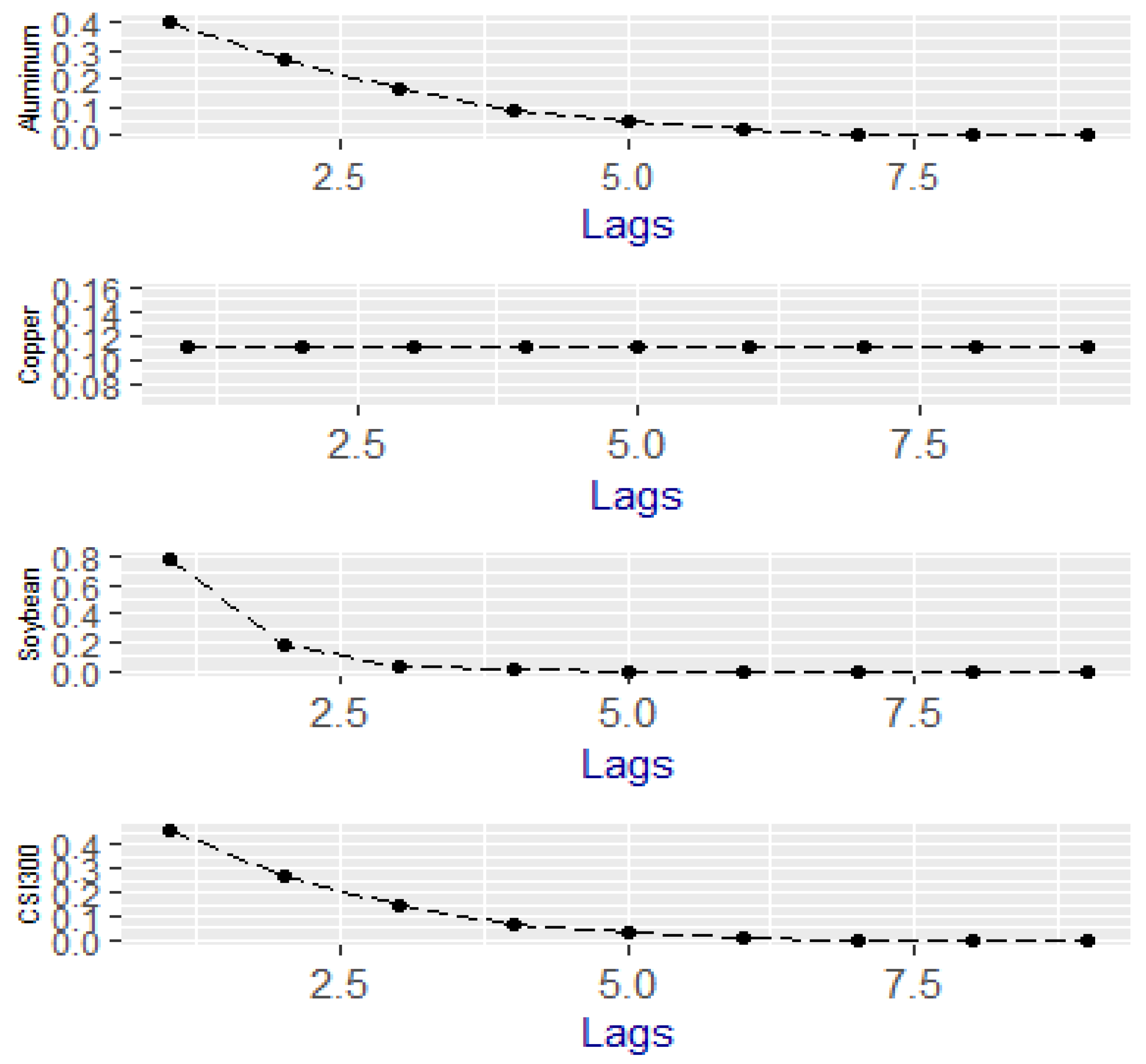
In the GARCH-MIDAS models with commodity futures, the sums of α and β are less than 1, which means the short-run variances in the commodities futures market has a lower persistence. Figure 3 illustrates the estimated exponential weights of the GARCH-MIDAS model with the fixed span RV for the 9-month lag. Figure 3 shows the optimal weights of the Aluminum, Soybean, and CSI 300. From Figure 3, we know the optimal weights of the four weights return decay with the increase of the lags.

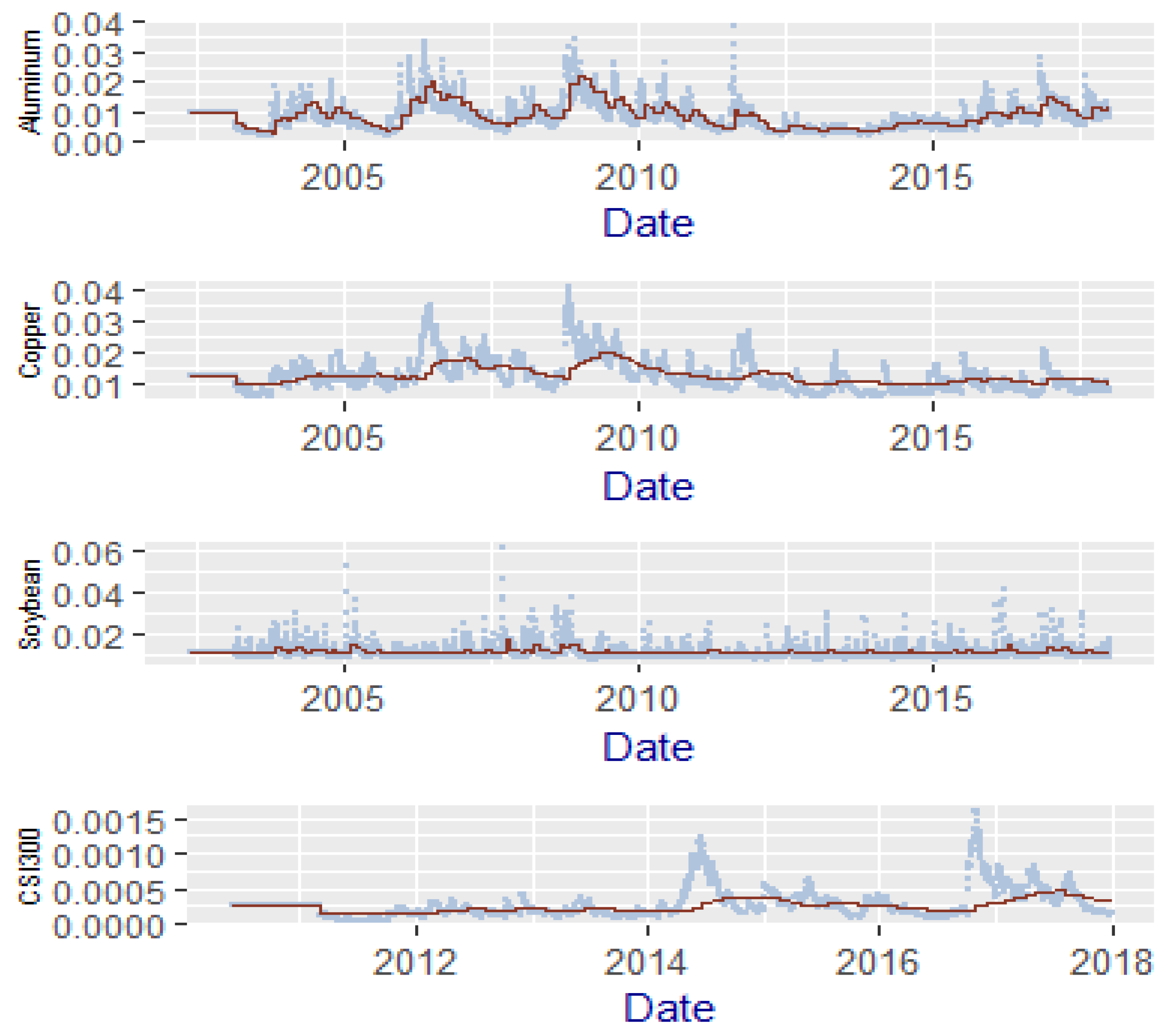
Figure 4 displays the different volatility components in the GARCH-MIDAS model with the fixed-span RV. The dashed lines are the conditional volatility in the futures market, while the solid lines stand for the secular component of the volatility in the GARCH-MIDAS model. In the GARCH-MIDAS model, the secular component is volatility, with the information of the lagging RV, and looks smoother.

Figure 3 illustrates the exponential lag weights for the GARCH-MIDAS model with fixed-span RV over the full sample period. The GARCH-MIDAS with monthly fixed-span RV uses nine lagged monthly RV in the MIDAS regression.

Figure 4 shows the estimated conditional variance and the secular component of GARCH-MIDAS model with monthly fixed RV in the MIDAS filter. In the GARCH-MIDAS model, we set the lag as 9. The solid line is the conditional variance and the dotted line is the long-run variance.

Table 5 illustrates the parameter estimates of the GARCH-MIDAS model is fitted with monthly fixed span RV. µ, α, β, θ and W are the parameters in the GARCH-MIDAS model. LLF, AIC, and BIC are the likelihood function value, AIC value, and BIC value. We set the lag is 9. The $\omega$ in the table is ${\omega }_2$, the optimal ${\omega }_1$ is 1. The numbers in parentheses are robust t-statistics computed with HAC standard errors.

3.2. Model with Macroeconomic Variables

How do macroeconomic fundamentals influence the volatility of futures returns? In this part, we try to answer the question. Schwert (1989), Engle and Rangel (2008), Engle et al. (2013) try to explain how much the macroeconomy affects the stock return volatility. Schwert (1989), Engle et al. (2013) employ the IP growth rate and PPI as the macroeconomic fundamentals and test the relationship between the macroeconomic variables and the stock market returns at monthly and quarterly horizons. Based on the references, we employ the IP, PPI, CPI, M2, and short-term interest rate as the macroeconomic fundamentals.

In the paper, we are interested in linking the daily futures return volatility with the monthly macroeconomic data. We start with the specifications involving the macroeconomic series, the level of IP, PPI, CPI, M2, and short-term interest rate. In the paper, we focus on the one-side filters. We employ the different weighting schemes to test the relationship between the level of macroeconomic series and the long-run variance. The parameter estimates of the GARCH-MIDAS model with the level of macroeconomic series are illustrated in

Table 6. Parameter estimates of one side GARCH-MIDAS model with consumer price index (CPI).

Futures	µ	α	β	θ	W	M
Aluminum	−0.000031	0.05	0.901	0.00017	4.99	0.000028
	(−0.31)	(25.31)	(246.59)	(3.99)	(0.78)	(19.12)
Copper	0.00029	0.075	0.91	0.0015	1.13	0.00014
	(1.63)	(15.53)	(198.52)	(2.28)	(0.93)	(5.68)
Soybean	0.000014	0.05	0.9	0.00015	4.99	0.00012
	(0.09)	(24.51)	(221.50)	(1.14)	(0.39)	(25.75)
CSI 300	0.00086	0.69	0.91	−0.0046	15.69	0.00036
	(2.79)	(7.63)	(73.69)	(−5.88)	(0.67)	(7.09)

,

Table 7. Parameter estimates of one side GARCH-MIDAS model with industrial production (IP).

Futures	µ	α	β	θ	W	M
Aluminum	−0.00009	0.093	0.9	−0.00063	3.17	0.00017
	(−1.13)	(31.72)	(425.63)	(−2.17)	(1.15)	(2.6)
Copper	0.00028	0.076	0.91	0.00085	1.05	0.00007
	(1.61)	(15.39)	(181.08)	(3.89)	(3.16)	(2.89)
Soybean	0.00018	0.2	0.62	−0.00041	23.1	0.00019
	(1.19)	(25.67)	(66.81)	(−8.35)	(0.49)	(22.64)
CSI 300	0.00086	0.069	0.91	−0.0031	3.77	0.00053
	(2.77)	(7.83)	(83.83)	−(4.73)	(0.86)	(5.49)

,

Table 8. Parameter estimates of one side GARCH-MIDAS model with producer price index (PPI).

Futures	µ	α	β	θ	W	M
Aluminum	−0.000078	0.072	0.92	0.00022	5	0.000048
	−(0.94)	(29.24)	(493.21)	(2.73)	(0.733)	(4.75)
Copper	0.00028	0.077	0.91	0.00011	1.01	0.00016
	(1.61)	(15.54)	(184.87)	(4.54)	(11.51)	(7.96)
Soybean	0.00012	0.19	0.62	0.00003	5.27	0.00014
	(0.87)	(24.81)	(69.54)	(1.04)	(0.18)	(36.1)
CSI 300	0.00086	0.068	0.92	−0.0019	3.63	0.00025
	(2.75)	(8.26)	(102.15)	(−3.47)	(0.99)	(5.03)

,

Table 9. Parameter estimates of one side GARCH-MIDAS model with money supply (M2).

Futures	µ	α	β	θ	W	M
Aluminum	−0.00006	0.079	0.9	0.00049	4.5	−4.7 × 10−5
	(−70.76)	(29.62)	(387.69)	(14.7)	(3.71)	(−13.82)
Copper	0.00028	0.075	0.91	0.0005	22.5	0.000096
	(1.57)	(15.54)	(194.56)	(2.26)	(0.13)	(2.7)
Soybean	0.00015	0.19	0.62	−0.00038	29.04	0.0002
	(1.05)	(25.13)	(66.21)	(−10.8)	(0.21)	(26.29)
CSI 300	0.0083	0.067	0.92	−0.004	36.03	0.0008
	(2.76)	(9.58)	(137.43)	(−3.51)	(0.12)	(3.66)

and

Table 10. Parameter estimates of one-side GARCH-MIDAS model with interest rate.

Futures	µ	α	β	θ	W	M
Aluminum	−0.000091	0.093	0.9	−0.0047	2.39	0.00011
	(−1.12)	(31.9)	(433.4)	(−1.23)	(0.21)	(2.52)
Copper	0.00028	0.077	0.9	0.28	1.64	0.00002
	(1.61)	(15.03)	(154.38)	(5.86)	(1.12)	(1.01)
Soybean	0.00013	0.19	0.63	−0.00074	25.71	0.00014
	(0.89)	(24.47)	(69.39)	(−0.77)	(0.0072)	(20.06)

.

Table 6 illustrates the parameter estimates of GARCH-MIDAS models with the level of CPI. For the specifications with macroeconomic level in the MIDAS filter, nine lags are taken into the GARCH-MIDAS model. The numbers in the parentheses are the t-statistics of the estimated parameters.

Table 7 illustrates the parameter estimates of GARCH-MIDAS models with the level of IP. For the specifications with macroeconomic level in the MIDAS filter, nine lags are taken into the GARCH-MIDAS model. The numbers in the parentheses are the t-statistics of the estimated parameters.

Table 8 illustrates the parameter estimates of GARCH-MIDAS models with the level of PPI. For the specifications with macroeconomic level in the MIDAS filter, nine lags are taken into the GARCH-MIDAS model. The numbers in the parentheses are the t-statistics of the estimated parameters.

Table 9 illustrates the parameter estimates of GARCH-MIDAS models with the level of M2. For the specifications with macroeconomic level in the MIDAS filter, nine lags are taken into the GARCH-MIDAS model. The numbers in the parentheses are the t-statistics of the estimated parameters.

Table 10 illustrates the parameter estimates of GARCH-MIDAS models with the interest rate level. The results of the GARCH-MIDAS model including the CSI 300 futures are parsimonious, and we only test the relationship between the commodity futures and interest rate. For specifications with macroeconomic level in the MIDAS filter, nine lags are taken into the GARCH-MIDAS model. The numbers in the parentheses are the t-statistics of the estimated parameters.

In Table 6, Table 7, Table 8, Table 9 and Table 10, the most notable parameters are the slope parameters of $\theta$ for the specification of the MIDAS filter. For the GARCH-MIDAS with the CPI time series, the $\theta$ ranges from 0.0015 to −0.0046. For the commodity futures, the slope parameters are positive; for the CSI 300 stock index futures, the $\theta$ is negative. From the t-statistics, we know the slope parameters are all statistically significant, which indicates the increase of the inflation level leads to a higher commodity futures return volatility. For the CSI 300 stock index futures, the increase of inflation level leads to a lower volatility of stock index futures return.

For Table 7, we can know the parameter estimates of the GARCH-MIDAS model with the industrial production index. The slope parameter $\theta$ ranges from −0.031 to 0.00085. For the aluminum futures, soybean futures, and CSI 300 stock index futures, the slope parameters are statistically negative, which means high-level industrial production decreases the return volatility in aluminum futures, soybean futures and the CSI 300 futures market. The increase in the output in manufacturing, mining, electric, and gas industry will decrease the aluminum futures, soybean futures, and CSI 300 futures return volatility. For copper futures, the slope parameter $\theta$ is positive, which indicates the increase in industrial production increases the copper futures return volatility.

Table 8 reports the GARCH-MIDAS with producer price index, the most interesting parameter $\theta$ ranges from −0.0019 to 0.00022. In all the GARCH-MIDAS model, the slope parameters are all statistically significant. For the commodity futures return, the increase of the PPI index leads to a higher commodity futures return volatility. For the GARCH-MIDAS model with CSI 300 futures return, the $\theta$ is significantly negative, which indicates the increase of the PPI index leads to a lower CSI 300 futures return volatility. The empirical results show that the increase in the selling price leads to a higher commodity futures return volatility. The increase in the selling price of the domestic producers decreases the CSI 300 futures return volatility.

Table 9 illustrates the GARCH-MIDAS model with M2. The slope parameter $\theta$ ranges from −0.004 to 0.0005. For the aluminum futures and the copper futures, the $\theta$ is statistically positive, which means the increase of money supply leads to a higher aluminum futures and copper futures return volatility. For the soybean futures and the CSI 300 stock futures, the slope parameters are negative, which illustrates the increase of the money supply decreases the futures return volatility in the soybean futures and CSI 300 futures market.

Table 10 shows the parameter estimates of the GARCH-MIDAS model with a short-term interest rate. As the parameter estimates of the stock index futures are parsimonious, Table 10 only reports the parameter estimates of the commodity futures. The parameter estimates of the $\theta$ in the GARCH-MIDAS model with short-term interest rate range from −0.0047 to 0.28. In all GARCH-MIDAS models with a short-term interest rate, the parameter estimates of $\theta$ are all statistically significant. For the aluminum futures and soybean futures, the slope parameters are negative, which means higher short-term interest rate leads to a lower aluminum and soybean futures return volatility. For the copper futures, the parameter estimates are 0.28 with a t-statistic of 5.86. The parameter estimates of $\theta$ indicates the higher short-term interest rates will increase the volatility in the Copper futures market.

In this part, we show the relationship between the level of macroeconomic variables and the futures return volatility. To examining the domestic macroeconomic determinants of the volatility of futures returns, we introduce the CPI, IP, PPI, M2, and short-term interest rate into the GARCH-MIDAS model. The research can be divided into two parts: the commodity futures and stock index futures. For the commodity futures market, the macroeconomic fundamentals have a different impact on the commodity futures volatility. CPI and PPI are the economic indicators, which measure the price fluctuations for goods and services. CPI measures expenditures of consumer-related services for residents. PPI evaluates the average changes in the sales prices for the entire domestic market of raw goods and services. M2 measures the money supply, including the elements of M1 and ‘near money.’

According to the empirical results, we can conclude two interesting results. First, based on the parameter estimates of $\theta$, we know that parameter estimates of $\theta$ in the GARCH-MIDAS model with CPI and PPI are all positive, which means the increase of the inflation in the market will lead to higher-level commodities futures return. Second, from Table 6, Table 7, Table 8 and Table 9 we know the parameter estimates of $\theta$ in the GARCH-MIDAS model with CSI 300 stock index futures are all negative. The empirical results illustrate that a high level of inflation, industrial production, and money supply will decrease the long-run variance in CSI stock index futures returns.

4. Conclusions

In this paper, we employ the GARCH-MIDAS model, which can decompose the conditional variance into the long-run and short-run component. The long-run component is decided by the MIDAS filter, and the short-run variance is decided by the GARCH model. In the research, we also link macroeconomic variables with the long-run volatility in the commodities futures market.

In the aluminum futures market, the increase of the CPI, PPI, and M2 level will increase the aluminum futures’ return volatility. The higher IP and short-term interest rate will lead to a lower futures return volatility in the aluminum futures market. From the empirical results, we can know the higher inflation in the economic market will increase the aluminum futures’ return volatility. The higher level of money supply will lead to higher return volatility in the aluminum futures market. The higher the price fluctuation for goods and services, the riskier the aluminum futures contracts will be. With the increase of the money supply, investors will spend more money to buy aluminum futures contracts. This also leads to riskier aluminum futures contracts. The higher level of output in the manufacturing, mining, and gas industries and higher industry and higher interest rate will lead to a less volatile aluminum futures market.

The macroeconomic variables have different impacts on the copper futures’ returns. The higher level of the CPI, PPI, M2, IP, and short-term interest rates lead to a less risky copper futures contract. The empirical results mean that the increase in inflation, money supply, short-term interest rate, and production level leads to a more volatile copper futures market. For the soybean futures market, the higher CPI and PPI will increase the returns’ volatility. The higher level of the IP, M2, and short-term interest rate will lead to a less risky soybean futures contracts.

The higher level of CPI and PPI will increase the return volatility in the soybean futures market. The increase of the IP, M2, and short-term interest rate will lead to lower futures return volatility in the soybean futures market. As an important agricultural product, soybean is highly related to the life of every consumer. Inflation will lead to high volatility in the soybean market and leads to volatile soybean futures contracts. The high-level CPI, IP, PPI, and M2 will lead to less risky CSI futures contracts. This illustrates that increasing inflation, money supply, and production will create a less volatile stock index futures market.

There are two implications from our results. First, our findings reveal strong evidence that the rise in inflation will lead to a more volatile commodity futures market. Second, an increase in inflation, production, and money supply will decrease the volatility of the CSI stock index futures’ return.

References

1. Arouri, Mohamed El Hedi, Jamel Jouini, and Duc Khuong Nguyen. 2011. Volatility spillovers between oil prices and stock sector returns: Implications for portfolio management. Journal of International Money and Finance 30: 1387–405. [Google Scholar] [CrossRef]
2. Asgharian, Hossein, Ai Jun Hou, and Farrukh Javed. 2013. Importance of the macroeconomic Variables for Variance Prediction: A GARCH-MIDAS Approach. Journal of Forecasting 32: 600–12. [Google Scholar] [CrossRef]
3. Barndorff-Nielsen, Ole E., and Neil Shephard. 2002. Econometric Analysis of Realized Volatility and Its Use in Estimating Stochastic Volatility Models. Journal of the Royal Statistical Society 64: 253–80. [Google Scholar] [CrossRef]
4. Batten, Jonathan A., Cetin Ciner, and Brian M. Lucey. 2010. The Macroeconomic Determinants of Volatility in Precious Metals Markets. Resources Policy 35: 65–71. [Google Scholar] [CrossRef]
5. Conrad, Christian, and Karin Loch. 2015. The variance risk premium and fundamental uncertainty. Economics Letters 132: 56–60. [Google Scholar] [CrossRef] [Green Version]
6. Dönmez, Ayca, and Emiliano Magrini. 2013. Agricultural Commodity Price Volatility and Its Macroeconomic Determinants: A GARCH-MIDAS Approach. JRC Working Papers JRC84138. Seville: Joint Research Centre. [Google Scholar]
7. Engle, Robert F., and Gary Lee. 1999. A permanent and transitory component model of stock return volatility. In Cointegration, Causality, and Forecasting: A Festschrift in Honor of Clive W.J. Granger. Edited by Robert Fry Engle and Halbert White. Oxford: Oxford University Press, pp. 475–97. [Google Scholar]
8. Engle, Robert F., and Jose Gonzalo Rangel. 2008. The Spline-GARCH Model for Low-Frequency Volatility and Its Global Macroeconomic Causes. The Review of Financial Studies 21: 1187–222. [Google Scholar] [CrossRef]
9. Engle, Robert F., Eric Ghysels, and Bumjean Sohn. 2013. Stock Market Volatility and Macroeconomic Fundamentals. Review of Economics and Statistics 95: 776–97. [Google Scholar] [CrossRef]
10. Fang, Libing, Honghai Yu, and Wen Xiao. 2018. Forecasting Gold Futures Market Volatility Using Macroeconomic Variables in the United States. Economic Modelling 72: 249–59. [Google Scholar] [CrossRef]
11. Frankel, Jeffrey A. 2014. Effects of Speculation and Interest Rates in a “carry trade” Model of Commodity Prices. Journal of International Money and Finance 42: 88–112. [Google Scholar] [CrossRef]
12. Ghosh, Dipak, Eric J. Levin, Peter Macmillan, and Robert E. Wright. 2004. Gold as an Inflation Hedge? Studies in Economics and Finance 22: 1–25. [Google Scholar] [CrossRef]
13. Ghysels, Eric, Arthur Sinko, and Rossen Valkanov. 2006. MIDAS regressions: Further Results and New Directions. Econometric Reviews 26: 53–90. [Google Scholar] [CrossRef]
14. Gorton, Gary, and Geert Rouwenhorst. 2006. Facts and Fantasies about Commodity Futures. Financial Analysts Journal 62: 47–68. [Google Scholar] [CrossRef] [Green Version]
15. Karali, Berna, and Gabriel J. Power. 2013. Short and Long-run Determinants of Commodity Price Volatility. American Journal of Agricultural Economics 95: 724–38. [Google Scholar] [CrossRef]
16. Karali, Berna, and Octavio A. Ramirez. 2014. Macro Determinants of Volatility and Volatility Spillover in Energy Markets. Energy Economics 46: 413–21. [Google Scholar] [CrossRef]
17. Mahdavi, Saeid, and Su Zhou. 1997. Gold and Commodity Prices as Leading Indicators of Inflation: Tests of Long-Run Relationship and Predictive Performance. Journal of Economics and Business 49: 475–89. [Google Scholar] [CrossRef]
18. Malik, Farooq, and Bradley T. Ewing. 2009. Volatility transmission between oil prices and equity sector returns. International Review of Financial Analysis 18: 95–100. [Google Scholar] [CrossRef]
19. Malik, Farooq, and Shawkat Hammoudeh. 2007. Shock and Volatility Transmission in the Oil, US and Gulf Equity Markets. International Review of Economics and Finance 16: 357–68. [Google Scholar] [CrossRef]
20. Merton, Robert C. 1980. On Estimating the Expected Return on the Market. Journal of Financial Economics 8: 323–61. [Google Scholar] [CrossRef]
21. Mo, Di, Rakesh Gupta, Bin Li, and Tarlok Singh. 2018. The Macroeconomic Determinants of Commodity Futures Volatility: Evidence from Chinese and Indian markets. Economic Modellingc 70: 543–60. [Google Scholar] [CrossRef]
22. Prokopczuk, Marcel, and Lazaros Symeonidis. 2013. The Economic Drivers of Time-Varying Commodity Market Volatility. Working Paper. Friedrichshafen: Zeppelin University. [Google Scholar]
23. Schwert, G. William. 1989. Why Does Stock Market Volatility Change over Time? The Journal of Finance 44: 1115–53. [Google Scholar] [CrossRef]
24. Thuraisamy, Kannan S., Susan Sunila Sharma, and Huson Joher Ali Ahmed. 2013. The Relationship between Asian Equity and Commodity Futures Markets. Journal of Asian Economics 28: 67–75. [Google Scholar] [CrossRef]
Figure 1. The price of the futures contract.
Ijfs 07 00063 g001
Figure 2. The log return of the futures contract.
Ijfs 07 00063 g002
Figure 3. Exponential weighting function.
Ijfs 07 00063 g003
Figure 4. The conditional variance and its secular component of a futures contract.
Ijfs 07 00063 g004