Relationship between Foreign Macroeconomic Conditions and Asian-Pacific Public Real Estate Markets: The Relative Influence of the US and China


Abstract
:1. Introduction
2. Brief Review and Literature Gap
3. Data
4. Research Methodology
4.1. Predictability of Macroeconomic Variables
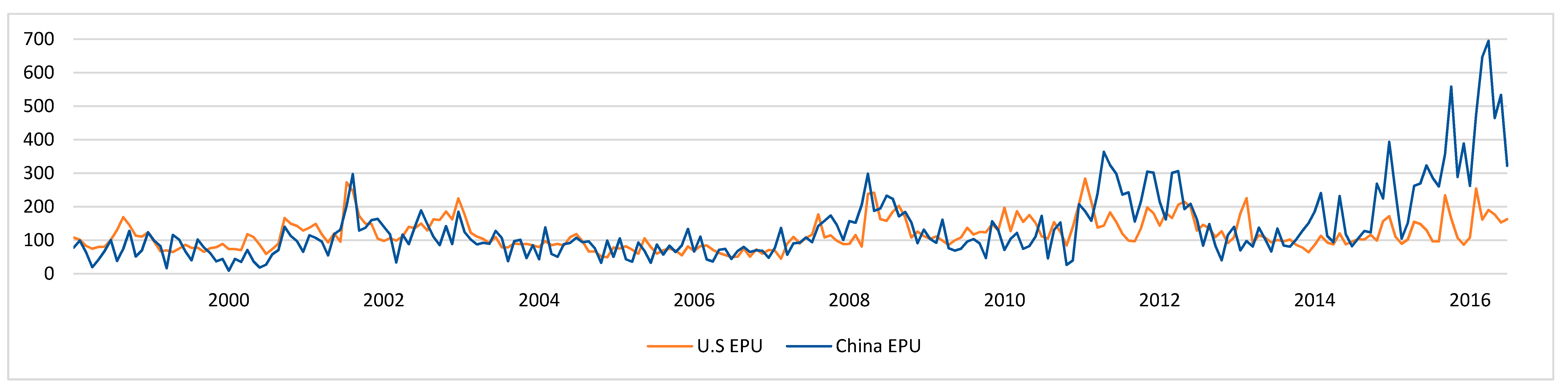
4.2. Predictability of Economic Policy Uncertainty (EPU)
4.3. Dynamic Linear and Non-Linear Causality between Macroeconomic Factors/EPU and Excess Returns
4.4. Generalized Impulse Response Functions
5. Results
5.1. Macroeconomic Factors and Excess Returns
5.2. EPU and Excess Returns
5.3. Linear Causality Interactions between the Foreign Macroeconomic Variables and APAC’s REERs
5.4. Linear Causality between EPU and REERs
5.5. Nonlinear Granger Causal Relations between APAC Nations’ REERs and US/CH Macroeconomic Conditions/EPU
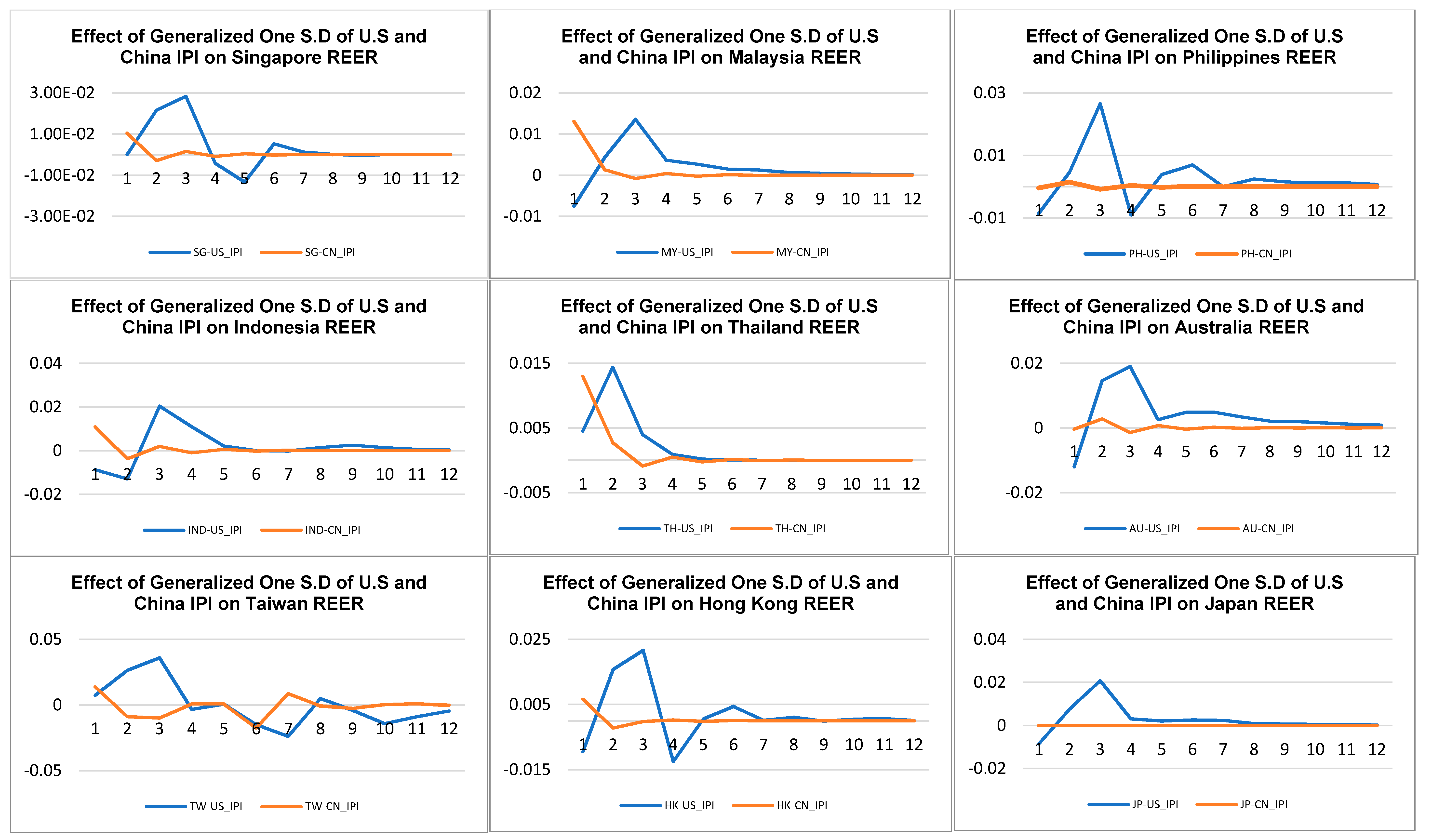
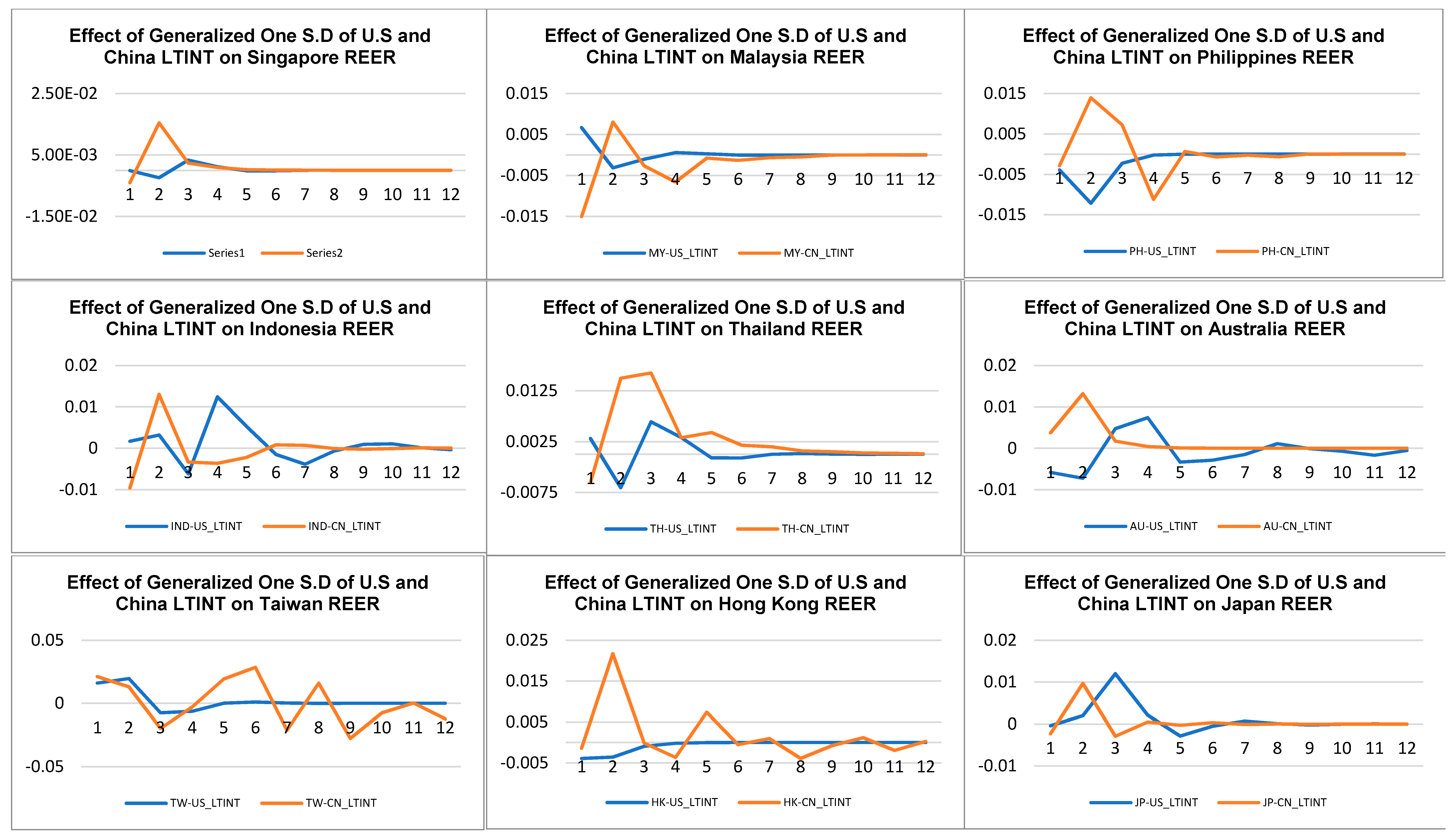
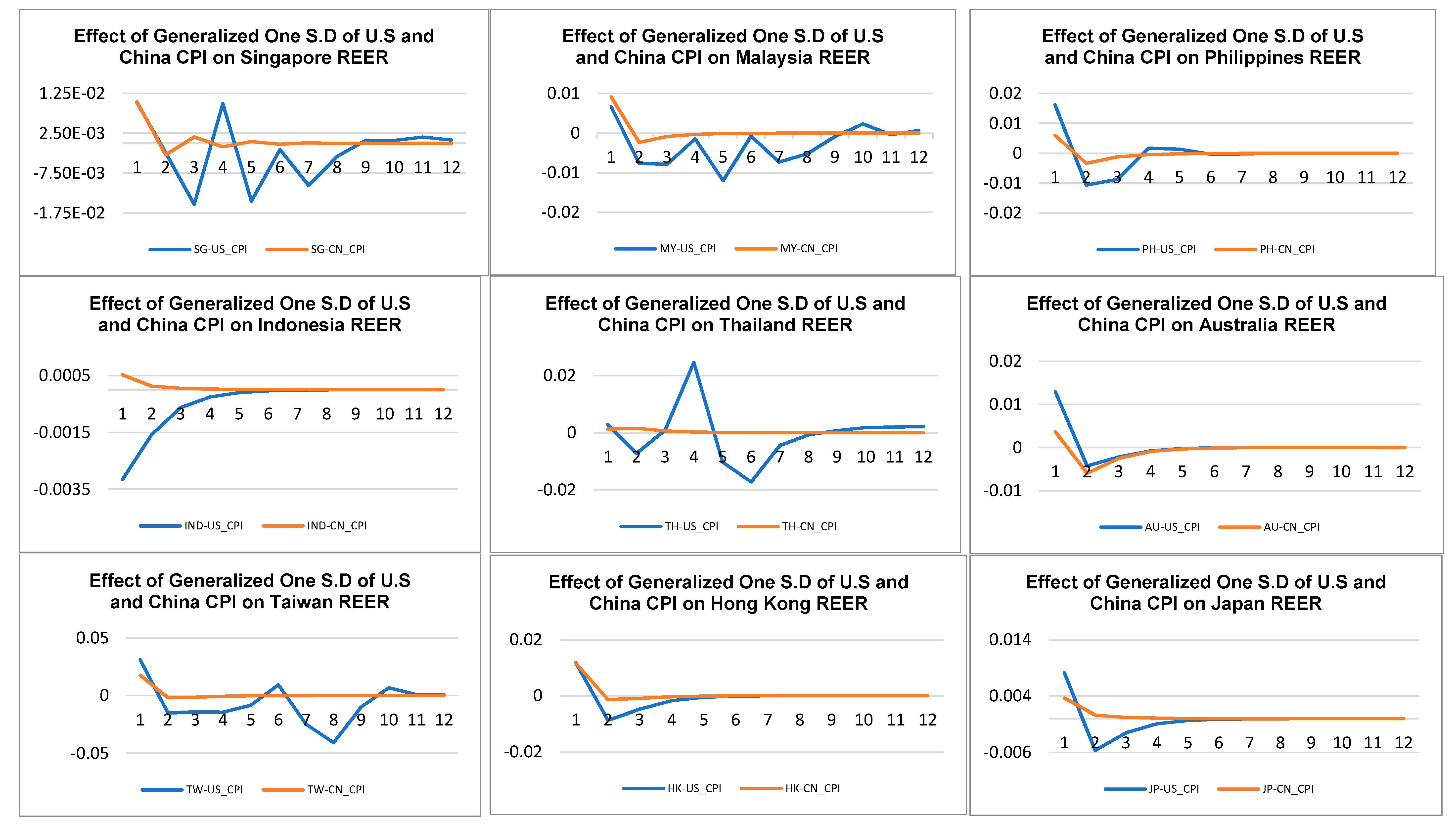
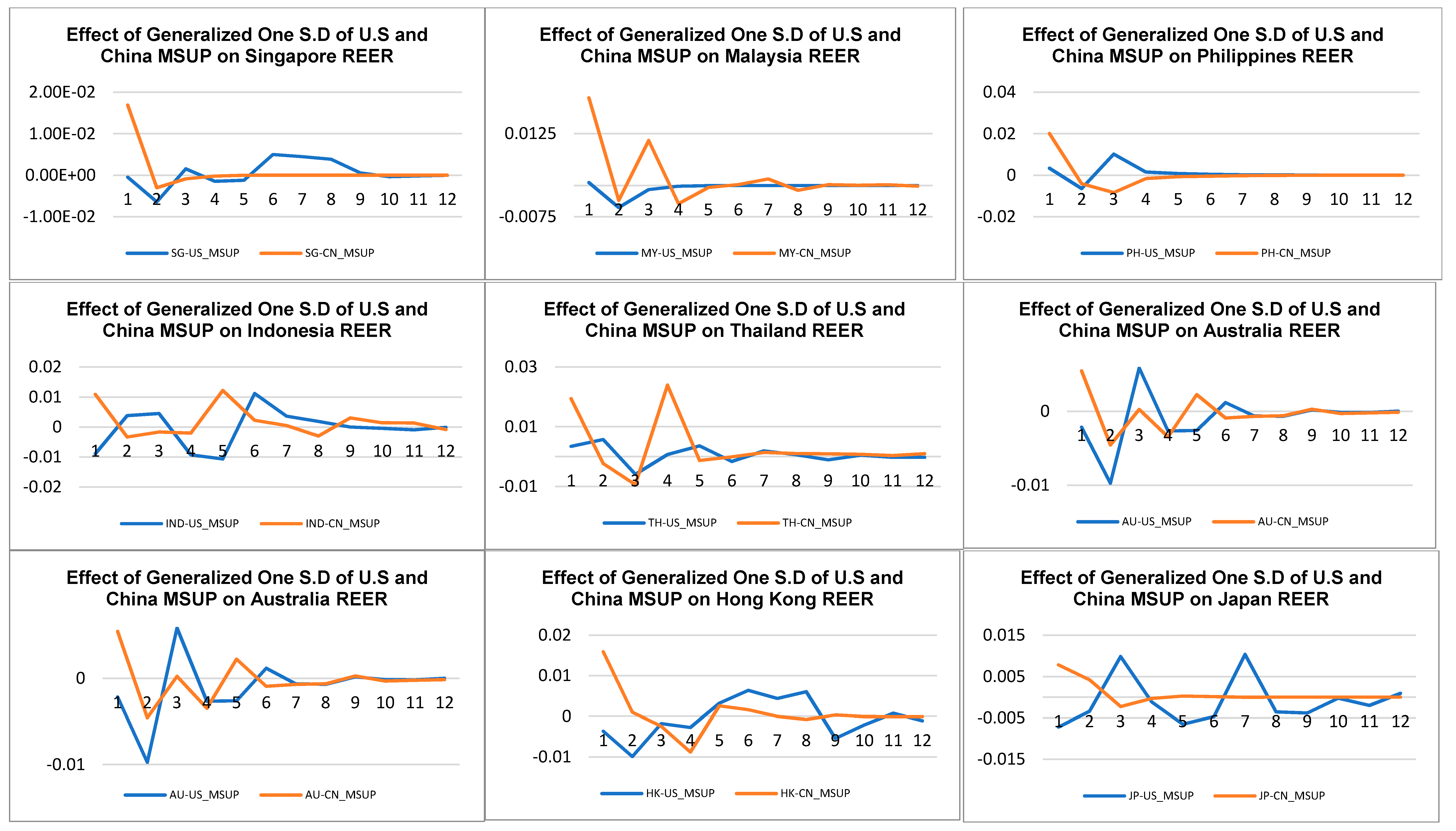
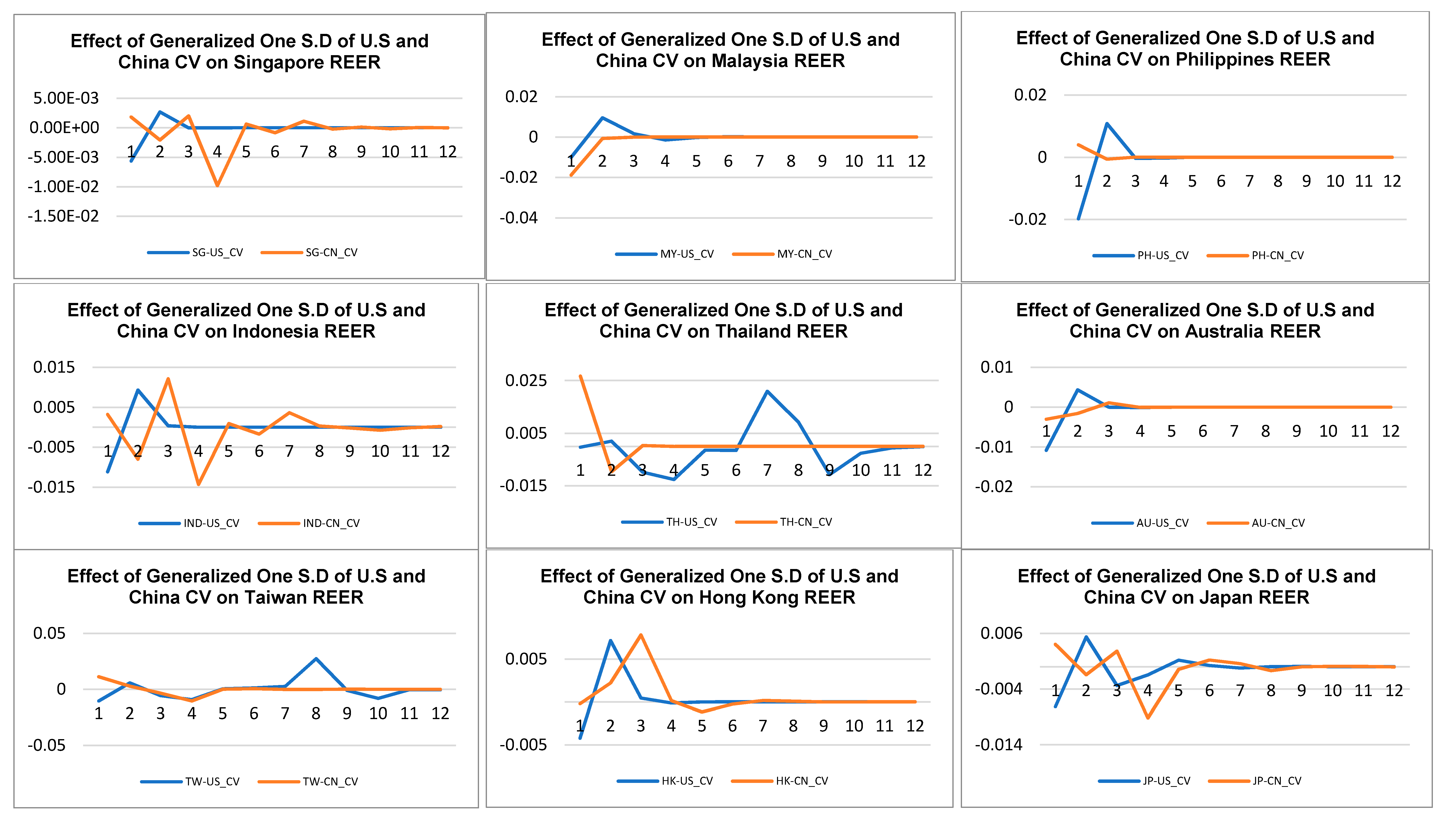
5.6. Impulse Response of Macroeconomic Factors/EPU on APAC Nations’ REERs
6. Conclusions
- Both US and China macroeconomic factors and economic policy uncertainty do not have any significant contemporaneous impact on APAC real estate market excess returns. These results agree with the conventional wisdom that foreign macroeconomic factors have weaker correlations with real estate returns, as compared to their domestic counterparts.
- The US and China macroeconomic factors and economic policy uncertainty Granger cause the APAC real estate market excess returns, although the causal effects are generally more prominent among the US macroeconomic factors using nonlinear causality tests. Additional findings affirm the expectation that China has an increasing influence over the APAC real estate markets examined over the short run while the US is still maintaining its dominance in the regional real estate markets in long run.
- The IRF analysis indicates that the shock response from the real estate excess returns in the ASEAN5 (part of APAC) is sensitive to both the US and China macroeconomic variables. In the context of regional globalization and financial market integration, ASEAN5 real estate markets are expected to be more interdependent with the US and China real estate markets.
Author Contributions
Funding
Conflicts of Interest
References
- Alam, Naushad. 2017. Analysis of the impact of select macroeconomic variables on the Indian stock market: A heteroscedastic cointegration approach. Business and Economic Horizons 13: 119–27. [Google Scholar] [CrossRef]
- Araújo, Eurilton. 2009. Macroeconomic shocks and the co-movement of stock returns in Latin America. Emerging Markets Review 10: 331–44. [Google Scholar] [CrossRef]
- Baek, Ehung Gi, and William A. Brock. 1992. A General Test for Nonlinear Granger Causality: Bivariate Model. Madison Working Paper. Ames: Iowa State Unoversity. [Google Scholar]
- Bailliu, Jeannine, and Patrick Blagrave. 2010. The Transmission of Shocks to the Chinese Economy in a Global Context: AModel-Based Approach. Working Paper 2010-07, July. Ottawa: Bank of Canada. [Google Scholar]
- Baker, Nicholas Bloom, and Steven J. Davis. 2016. Measuring economic policy uncertainty. The Quarterly Journal of Economics 131: 1593–636. [Google Scholar] [CrossRef]
- Binswanger, Mathias. 2004. How important are fundamentals? Evidence from a structural VAR model for the stock markets in US, Japan and Europe. Journal of International Financial Markets Institutions and Money 14: 185–201. [Google Scholar] [CrossRef]
- Bloom, Nicholas. 2009. The impact of uncertainty shocks. Econometrica 77: 623–85. [Google Scholar]
- Chan, Kam C., Benton E. Gup, and Ming-Shiun Pan. 1992. An Empirical Analysis of Stock Prices in Major Asian Markets and the United States. The Financial Review 27: 289–307. [Google Scholar] [CrossRef]
- Chen, Nai-Fu, Richard Roll, and Stephen A. Ross. 1986. Economic forces and the stock market. Journal of Business 59: 383–403. [Google Scholar] [CrossRef]
- Chen, Jian, Fuwei Jiang, and Guoshi Tong. 2016. Economic Policy Uncertainty in China and Stock Market Expected Returns. Accounting & Finance 57: 1265–86. [Google Scholar]
- Cheng, Hwahsin, and John L. Glascock. 2006. Stock market linkages before and after the Asian financial Crisis: Evidence from three Greater China economic area stock markets and the US. Review of Pacific Basin Financial Markets and Policies 9: 297–306. [Google Scholar] [CrossRef]
- Cheng, Andy, and Iris Wing Han Yip. 2017. China’s macroeconomic fundamentals on stock market volatility: Evidence from Shanghai and Hong Kong. Review of Pacific Basin Financial Markets and Policies 20: 1–57. [Google Scholar] [CrossRef]
- Diks, Cees, and Valentyn Panchenko. 2006. A new statistic and practical guidelines for nonparametric Granger causality testing. Journal of Economic Dynamics and Control 30: 1647–69. [Google Scholar] [CrossRef]
- Donadelli, Michael. 2015. Asian stock markets, US economic policy uncertainty and US macro shocks. New Zealand Economic Papers 49: 103–33. [Google Scholar] [CrossRef]
- Donadelli, Michael, and Lauren Persha. 2014. Understanding emerging market equity risk premia: Industries, governance and macroeconomic policy uncertainty. Research in International Business and Finance 30: 284–309. [Google Scholar] [CrossRef]
- Donadelli, Michael, and Lorenzo Prosperi. 2012. On the role of liquidity in emerging markets stock prices. Research in Economics 66: 320–48. [Google Scholar] [CrossRef]
- Eickmeier, Sandra, and Markus Kuhnlenz. 2013. China’s Role in Global Inflation Dynamics. Bundesbank Discussion Paper 07/2013. Cambridge: Cambridge University Press. [Google Scholar]
- Fama, Eugene F. 1981. Stock returns, real activity, inflation and money. American Economic Review 71: 545–65. [Google Scholar]
- Fung, Hung-Gay, Guoming Huang, Qingfeng Liu, and Xiaoqin Shen. 2006. The development of the real estate industry in China. The Chinese Economy 39: 84–102. [Google Scholar] [CrossRef]
- Granger, Clive W. J. 1969. Investigating causal relations by econometric models and cross-spectral methods. Econometrica 37: 424–38. [Google Scholar] [CrossRef]
- Hiemstra, Craig, and Jonathan D. Jones. 1994. Testing for linear and nonlinear Granger causality in the stock price-volume relation. Journal of Finance 49: 1639–64. [Google Scholar]
- Hui, Eddie C. M., and Ivan M. H. Ng. 2012. Wealth effect, credit price effect, and the relationships between Hong Kong property market and stock market. Property Management 30: 255–73. [Google Scholar] [CrossRef]
- International Monetary Fund. 2017. Regional Economic Outlook: Asia Pacific: Preparing for Choppy Seas, May. Washington: International Monetary Fund. [Google Scholar]
- Johansson, Anders C., and Christer Ljungwall. 2009. Spillover effects among the Greater China stock markets. World Development 37: 839–51. [Google Scholar] [CrossRef]
- Li, Xiao-Lin, Mehmet Balcilar, Rangan Gupta, and Tsangyao Chang. 2015. The causal relationship between economic policy uncertainty and stock returns in China and India: Evidence from a bootstrap rolling window approach. Emerging Markets Finance and Trade 52: 674–89. [Google Scholar] [CrossRef]
- Ling, David C., and Andy Naranjo. 2002. Commercial real estate return performance: A cross-country analysis. Journal of Real Estate Finance and Economics 24: 119–42. [Google Scholar] [CrossRef]
- Liow, Kim Hiang, and Alastair Adair. 2009. Do Asian real estate companies add value to investment portfolio? Journal of Property Investment & Finance 27: 42–64. [Google Scholar]
- Narayan, Paresh Kumar, and Seema Narayan. 2012. Do US macroeconomic conditions affect Asian stock market returns? Journal of Asian Economics 23: 669–79. [Google Scholar] [CrossRef]
- Nikkinen, Jussi, and Petri Sahlstrom. 2004. Scheduled domestic and US macroeconomic news and stock valuation in Europe. Journal of Multinational Financial Management 14: 201–15. [Google Scholar] [CrossRef]
- Nishimura, Yusaku, and Ming Men. 2010. The paradox of China’s international stock market co-movement: Evidence from volatility spillover effects between China and G5 stock markets. Journal of Chinese Economic and Foreign Trade Studies 3: 235–53. [Google Scholar] [CrossRef]
- Okunev, John, Patrick Wilson, and Ralf Zurbruegg. 2000. The causal relationship between real estate and stock markets. The Journal of Real Estate Finance and Economics 21: 251–61. [Google Scholar] [CrossRef]
- Pesaran, H. Hashem, and Yongcheol Shin. 1998. Generalized impulse response analysis in linear multivariate models. Economics Letters 58: 17–29. [Google Scholar] [CrossRef]
- Roll, Richard, and Stephen A. Ross. 1980. An empirical investigation of the arbitrage pricing theory. Journal of Finance 35: 1073–103. [Google Scholar] [CrossRef]
- Ross, Stephen A. 1976. The arbitrage pricing theory of capital asset pricing. Journal of Economic Theory 13: 341–60. [Google Scholar] [CrossRef]
- Schindler, Felix. 2011. Long-term benefits from investing in international securitized real estate. International Real Estate Review 14: 27–60. [Google Scholar]
- Sharma, Subhash C., and Praphan Wongbangpo. 2002. Stock market and macroeconomic fundamental dynamic interactions: ASEAN-5 countries. Journal of Asian Economics 13: 27–51. [Google Scholar]
- Sum, Vichet. 2013. The ASEAN Stock Market Performance and Economic Policy Uncertainty in the United States. Economic Papers: Journal of Applied Economics and Policy 32: 512–21. [Google Scholar] [CrossRef]
- Zheng, Yongnianand, and Chi Zhang. 2016. The Belt and Road Initiative and China’s Grand Diplomacy. China and the World 1: 309–31. [Google Scholar]
| 1 | Real estate investments exist in two main forms: Private real estate and public real estate. While the former refers to physical properties with steady cash flows, the latter is a more liquid and low-cost channel to gain real estate exposure, such as listed real estate companies and real estate investment trusts (known as REITs). Public real estate (the subject of this study) is also commonly referred as “securitized real estate”. From this point onward, the terms “securitized real estate”, “public real estate”, and “real estate” will be used interchangeably throughout the text. |
| 2 | MSCI stands for Morgan Stanley Capital International. |
| 3 | The sub-period results are not reported in order to conserve space. |
| 4 | As highlighted in Footnote 1, this study is concerned with public real estate (securitized real estate), which is part of the stock market and an important asset component in many national economies. As documented in many real estate studies (Fung et al. 2006; Schindler 2011; Ling and Naranjo 2002), since direct (physical) real estate usually respond more slowly to economic stimuli than other financial markets (usually up to three-month lags), it is adequate to assume traded (or public) real estate responds faster, only between one- and two-month delays. |


| Country. | Mean | Std. Deviation | Kurtosis | Skewness | Sharpe Ratio |
|---|---|---|---|---|---|
| Singapore | 0.001 | 0.112 | 7.141 | −0.095 | 0.006 |
| Malaysia | −0.003 | 0.109 | 6.077 | −0.061 | −0.024 |
| Philippines | 0.005 | 0.11 | 4.326 | −0.226 | 0.042 |
| Indonesia | −0.015 | 0.214 | 20.536 | −0.717 | −0.069 |
| Thailand | 0.006 | 0.189 | 44.21 | 4.18 | 0.029 |
| Australia | −0.001 | 0.072 | 13.995 | −2.151 | −0.01 |
| Taiwan | −0.006 | 0.162 | 45.014 | 4.214 | −0.037 |
| Hong Kong | 0.002 | 0.101 | 6.403 | 0.029 | 0.023 |
| Japan | 0.002 | 0.087 | 3.783 | 0.226 | 0.018 |
| Variable | Definition and Description | Expected Sign |
|---|---|---|
| Industrial Production Index (IPI) | It measures the changes in the real output primarily in the manufacturing sector of an economy, relative to a base year. A higher level of IPI indicates higher productivity of the underlying economy and hence will enhance the return performance of real estate assets. | + |
| Long-Term Interest Rate (LTINT) | It refers to the government bond yield with a maturity of 10 years or more. These interest rates are implied by the prices at which the government bonds are traded on financial markets. It is one of the key determinants of investments. With lower interest costs, investment activities may be more attractive, which in turn boost economic growth. | − |
| Consumer Price Index (CPI) | An important economic indicator to measure the level of inflation in an economy. With higher inflation, it will erode the purchasing power of consumers as well as the overall returns on assets. | − |
| Money Supply (MS) | It has an inverse relationship between interest rates. With more money circulating in the economy, it will stimulate investments and will spur economic growth. | + |
| Conditional Variance (CV) | CV quantifies our uncertainty about the future observation, given everything we have seen so far. It is more practical as a forecast than the volatility of the entire series considered in the capital markets. | − |
| Economic Policy Uncertainty (EPU) | A macroeconomic risk indicator that takes into account the uncertainty in policies drafted by government agencies and news reported relating to events of economic uncertainties. | − |
| US risk factors: summary statistics | |||||
| Variable | Symbol | Mean | Std. Dev. | ||
| US macroeconomic variables | |||||
| Change in US Industrial Production Index | IPI | 0.001 | 0.007 | ||
| Change in US Long-Term Interest Rate | LTINT | −0.004 | 0.053 | ||
| Change in US Consumer Price Index | CPI | 0.002 | 0.003 | ||
| Change in US Money Supply Aggregate | MS | 0.000 | 0.099 | ||
| Change in US Conditional Volatility | CV | −0.003 | 0.470 | ||
| US risk factors: correlation matrix | |||||
| Variable | IPI | LTINT | CPI | MS | CV |
| IPI | 1.000 | ||||
| LTINT | 0.055 | 1.000 | |||
| CPI | 0.081 | 0.265 | 1.000 | ||
| MS | −0.128 | −0.119 | −0.027 | 1.000 | |
| CV | 0.050 | −0.073 | −0.243 | 0.092 | 1.000 |
| China risk factors: summary statistics | |||||
| Variable | Symbol | Mean | Std. Dev. | ||
| China macroeconomic variables | |||||
| Change in China Industrial Production Index | IPI | 0.002 | 0.040 | ||
| Change in China Long-Term Interest Rate | LTINT | −0.004 | 0.002 | ||
| Change in China Consumer Price Index | CPI | 0.012 | 0.003 | ||
| Change in China Money Supply Aggregate | MS | 0.014 | 0.013 | ||
| Change in China Conditional Volatility | CV | 0.197 | 0.470 | ||
| China risk factors: correlation matrix | |||||
| Variable | IPI | LTINT | CPI | MS | CV |
| IPI | 1.000 | ||||
| LTINT | 0.051 | 1.000 | |||
| CPI | 0.203 | 0.084 | 1.000 | ||
| MS | 0.256 | 0.020 | 0.740 | 1.000 | |
| CV | −0.002 | 0.094 | 0.055 | 0.032 | 1.000 |
| Panel A: US | |||||||
|---|---|---|---|---|---|---|---|
| IPI | LTINT | CPI | MS | CV | |||
| Country | Constant | β1IPIt−1 | β2LTINTt−1 | β3CPIt−1 | β4MSt−1 | β5CVt−1 | R2 |
| Singapore | −0.002 | −0.292 | −0.03 | 2.149 | 0.003 | −0.01 | 0.007 |
| Malaysia | −0.001 | −0.412 | 0.093 | −0.334 | −0.009 | −0.023 | 0.016 |
| Philippines | −0.001 | −0.274 | −0.176 | 2.22 | 0.052 | −0.040 ** | 0.043 |
| Indonesia | −0.008 | −0.043 | 0.016 | −1.962 | −0.048 | −0.029 | 0.007 |
| Thailand | 0.004 | 1.313 | 0.033 | −0.982 | 0.099 | 0.003 | 0.005 |
| Australia | −0.008 | −0.588 | −0.203 ** | 3.771 ** | −0.048 | −0.018 * | 0.061 |
| Taiwan | −0.014 | −0.346 | 0.288 | 5.51 | −0.026 | −0.018 | 0.031 |
| Hong Kong | −0.003 | −1.177 | −0.118 | 3.281 | −0.04 | −0.012 | 0.023 |
| Japan | −0.001 | −0.514 | −0.087 | 1.503 | −0.028 | −0.016 | 0.016 |
| China + | 0.006 | −1.443 | −0.134 | −0.083 | 0.018 | −0.016 | 0.016 |
| Panel B: China | |||||||
| IPI | LTINT | CPI | MS | CV | |||
| Country | Constant | β1IPIt−1 | β2LTINTt−1 | β3CPIt−1 | β4MSt−1 | β5CVt−1 | R2 |
| Singapore | −0.01 | 0.089 | 0.004 | 0.021 | 0.959 | −0.014 | 0.03 |
| Malaysia | −0.039 *** | −0.004 | −0.176 | −1.626 ** | 3.085 *** | −0.047 | 0.17 |
| Philippines | −0.013 | −0.24 | 0.032 | −1.058 | 1.878 ** | −0.019 | 0.041 |
| Indonesia | −0.005 | 0.13 | −0.193 | 1.556 * | −0.484 | −0.004 | 0.037 |
| Thailand | 0.003 | 0.015 | −0.015 | 0.216 | 0.147 | 0.018 | 0.003 |
| Australia | −0.006 | −0.123 | 0.1 | −0.334 | 0.548 | −0.027 | 0.014 |
| Taiwan | −0.041 ** | 0.073 | 0.458 * | −1.747 | 3.404 ** | 0.01 | 0.06 |
| Hong Kong | −0.015 | 0.01 | −0.016 | −0.089 | 1.318 ** | −0.018 | 0.049 |
| Japan | −0.008 | −0.025 | −0.043 | −0.615 | 1.009 | −0.01 | 0.016 |
| US + | −0.004 | −0.032 | −0.235 | −0.086 | −0.249 | −0.086 *** | 0.074 |
| Panel A: US | ||||
|---|---|---|---|---|
| EPU | WORLD | |||
| Country | Constant | β6EPUt−1 | β7WORLDt | R2 |
| Singapore | 0.055 | −0.013 | 1.384 *** | 0.334 |
| Malaysia | −0.04 | 0.008 | 0.671 *** | 0.08 |
| Philippines | −0.149 | 0.033 | 1.311 *** | 0.301 |
| Indonesia | 0.067 | −0.018 | 0.631 ** | 0.02 |
| Thailand | −0.136 | 0.031 | 1.143 *** | 0.078 |
| Australia | 0.026 | −0.007 | 0.978 *** | 0.408 |
| Taiwan | 0.065 | −0.016 | 1.008 *** | 0.087 |
| Hong Kong | −0.008 | 0.001 | 1.261 *** | 0.332 |
| Japan | −0.006 | 0.001 | 0.844 *** | 0.203 |
| China + | 0.153 | −0.033 | 0.369 ** | 0.031 |
| Panel B: China | ||||
| EPU | WORLD | |||
| Country | Constant | β6EPUt−1 | β7WORLDt | R2 |
| Singapore | −0.019 | 0.003 | 1.398 *** | 0.333 |
| Malaysia | −0.028 | 0.005 | 0.669 *** | 0.08 |
| Philippines | −0.083 ** | 0.018 ** | 1.30 *** | 0.305 |
| Indonesia | −0.067 | 0.011 | 0.657 ** | 0.021 |
| Thailand | −0.16 | 0.035 ** | 1.152 *** | 0.091 |
| Australia | −0.031 | 0.006 | 0.990 *** | 0.411 |
| Taiwan | −0.079 | 0.015 | 1.036 *** | 0.09 |
| Hong Kong | −0.031 | 0.006 | 1.265 *** | 0.334 |
| Japan | −0.005 | 0.001 | 0.844 *** | 0.203 |
| US + | −0.084 ** | 0.014 * | 0.007 | 0.016 |
| US Macroeconomic Variables | Test Values | Test Values | |||||||||
|---|---|---|---|---|---|---|---|---|---|---|---|
| Null Hypothesis | F-Value | p-Value | Country | Null Hypothesis | F-Value | p-Value | |||||
| SG | (IPI) | ≠> | (REER) | 4.133 | 0.017 ** | MY | (IPI) | ≠> | (REER) | 2.136 | 0.097 * |
| (REER) | ≠> | (LPI) | 7.061 | 0.001 *** | (REER) | ≠> | (LPI) | 2.661 | 0.049 ** | ||
| (LINT) | ≠> | (REER) | 6.951 | 0.001 *** | (LINT) | ≠> | (REER) | 3.313 | 0.021 ** | ||
| (REER) | ≠> | (LINT) | 0.18 | 0.835 | (REER) | ≠> | (LINT) | 0.347 | 0.791 | ||
| (CPI) | ≠> | (REER) | 5.043 | 0.007 *** | (CPI) | ≠> | (REER) | 0.822 | 0.483 | ||
| (REER) | ≠> | (CPI) | 0.938 | 0.393 | (REER) | ≠> | (CPI) | 0.822 | 0.483 | ||
| (MS) | ≠> | (REER) | 1.254 | 0.287 | (MS) | ≠> | (REER) | 0.867 | 0.459 | ||
| (REER) | ≠> | (MS) | 0.548 | 0.58 | (REER) | ≠> | (MS) | 0.353 | 0.787 | ||
| (CV) | ≠> | (REER) | 15.86 | 0.000 *** | (CV) | ≠> | (REER) | 3.162 | 0.025 ** | ||
| (REER) | ≠> | (CV) | 0.479 | 0.62 | (REER) | ≠> | (CV) | 1.016 | 0.386 | ||
| PH | (IPI) | ≠> | (REER) | 3.895 | 0.022 ** | IND | (IPI) | ≠> | (REER) | 0.829 | 0.479 |
| (REER) | ≠> | (LPI) | 7.791 | 0.001 *** | (REER) | ≠> | (LPI) | 1.606 | 0.189 | ||
| (LINT) | ≠> | (REER) | 3.253 | 0.041 ** | (LINT) | ≠> | (REER) | 0.407 | 0.748 | ||
| (REER) | ≠> | (LINT) | 1.118 | 0.329 | (REER) | ≠> | (LINT) | 0.624 | 0.6 | ||
| (CPI) | ≠> | (REER) | 0.707 | 0.494 | (CPI) | ≠> | (REER) | 0.302 | 0.824 | ||
| (REER) | ≠> | (CPI) | 1.662 | 0.192 | (REER) | ≠> | (CPI) | 0.052 | 0.984 | ||
| (MS) | ≠> | (REER) | 0.605 | 0.547 | (MS) | ≠> | (REER) | 1.394 | 0.246 | ||
| (REER) | ≠> | (MS) | 1.509 | 0.223 | (REER) | ≠> | (MS) | 0.386 | 0.763 | ||
| (CV) | ≠> | (REER) | 8.667 | 0.000 *** | (CV) | ≠> | (REER) | 3.472 | 0.017 ** | ||
| (REER) | ≠> | (CV) | 1.633 | 0.198 | (REER) | ≠> | (CV) | 0.88 | 0.452 | ||
| TH | (IPI) | ≠> | (REER) | 3.538 | 0.031 ** | AU | (IPI) | ≠> | (REER) | 24.25 | 0.000 *** |
| (REER) | ≠> | (LPI) | 2.935 | 0.055 * | (REER) | ≠> | (LPI) | 18.12 | 0.000 *** | ||
| (LINT) | ≠> | (REER) | 2.089 | 0.126 | (LINT) | ≠> | (REER) | 6.334 | 0.013 ** | ||
| (REER) | ≠> | (LINT) | 0.323 | 0.724 | (REER) | ≠> | (LINT) | 0.547 | 0.46 | ||
| (CPI) | ≠> | (REER) | 1.927 | 0.148 | (CPI) | ≠> | (REER) | 17.04 | 0.000 *** | ||
| (REER) | ≠> | (CPI) | 0.605 | 0.547 | (REER) | ≠> | (CPI) | 1.28 | 0.259 | ||
| (MS) | ≠> | (REER) | 0.245 | 0.783 | (MS) | ≠> | (REER) | 0.03 | 0.863 | ||
| (REER) | ≠> | (MS) | 0.278 | 0.757 | (REER) | ≠> | (MS) | 4.515 | 0.035 ** | ||
| (CV) | ≠> | (REER) | 3.258 | 0.040 ** | (CV) | ≠> | (REER) | 42.7 | 0.000 *** | ||
| (REER) | ≠> | (CV) | 1.338 | 0.265 | (REER) | ≠> | (CV) | 1.159 | 0.283 | ||
| TW | (IPI) | ≠> | (REER) | 6.062 | 0.000 *** | HK | (IPI) | ≠> | (REER) | 4.051 | 0.008 *** |
| (REER) | ≠> | (LPI) | 2.142 | 0.096 | (REER) | ≠> | (LPI) | 7.284 | 0.000 *** | ||
| (LINT) | ≠> | (REER) | 0.969 | 0.381 | (LINT) | ≠> | (REER) | 10.1 | 0.002 *** | ||
| (REER) | ≠> | (LINT) | 1.785 | 0.17 | (REER) | ≠> | (LINT) | 0.266 | 0.607 | ||
| (CPI) | ≠> | (REER) | 3.469 | 0.064 * | (CPI) | ≠> | (REER) | 13.5 | 0.000 *** | ||
| (REER) | ≠> | (CPI) | 2.389 | 0.124 | (REER) | ≠> | (CPI) | 2.736 | 0.100 * | ||
| (MS) | ≠> | (REER) | 5.026 | 0.000 *** | (MS) | ≠> | (REER) | 0.386 | 0.68 | ||
| (REER) | ≠> | (MS) | 0.93 | 0.493 | (REER) | ≠> | (MS) | 0.925 | 0.398 | ||
| (CV) | ≠> | (REER) | 2.964 | 0.004 *** | (CV) | ≠> | (REER) | 34.7 | 0.000 *** | ||
| (REER) | ≠> | (CV) | 0.998 | 0.439 | (REER) | ≠> | (CV) | 1.588 | 0.209 | ||
| JP | (IPI) | ≠> | (REER) | 5.706 | 0.004 *** | ||||||
| (REER) | ≠> | (LPI) | 8.462 | 0.000 *** | |||||||
| (LINT) | ≠> | (REER) | 6.289 | 0.002 *** | |||||||
| (REER) | ≠> | (LINT) | 2.487 | 0.086 * | |||||||
| (CPI) | ≠> | (REER) | 10.359 | 0.002 *** | |||||||
| (REER) | ≠> | (CPI) | 1.252 | 0.264 | |||||||
| (MS) | ≠> | (REER) | 2.004 | 0.137 | |||||||
| (REER) | ≠> | (MS) | 0.802 | 0.45 | |||||||
| (CV) | ≠> | (REER) | 3.32 | 0.021 ** | |||||||
| (REER) | ≠> | (CV) | 1.511 | 0.213 | |||||||
| Test Values | Test Values | ||||||||||
|---|---|---|---|---|---|---|---|---|---|---|---|
| Null Hypothesis | F-Value | p-Value | Null Hypothesis | F-Value | p-Value | ||||||
| SG | (IPI) | ≠> | (REER) | 1.569 | 0.212 | MY | (IPI) | ≠> | (REER) | 1.376 | 0.242 |
| (REER) | ≠> | (LPI) | 0.264 | 0.608 | (REER) | ≠> | (LPI) | 0.064 | 0.801 | ||
| (LINT) | ≠> | (REER) | 9.195 | 0.003 *** | (LINT) | ≠> | (REER) | 6.872 | 0.000 *** | ||
| (REER) | ≠> | (LINT) | 6.599 | 0.011 ** | (REER) | ≠> | (LINT) | 1.005 | 0.392 | ||
| (CPI) | ≠> | (REER) | 1.569 | 0.212 | (CPI) | ≠> | (REER) | 1.588 | 0.209 | ||
| (REER) | ≠> | (CPI) | 0.264 | 0.608 | (REER) | ≠> | (CPI) | 0.122 | 0.728 | ||
| (MS) | ≠> | (REER) | 0.764 | 0.383 | (MS) | ≠> | (REER) | 0.969 | 0.426 | ||
| (REER) | ≠> | (MS) | 0.24 | 0.624 | (REER) | ≠> | (MS) | 1.393 | 0.237 | ||
| (CV) | ≠> | (REER) | 2.448 | 0.119 | (CV) | ≠> | (REER) | 0.093 | 0.761 | ||
| (REER) | ≠> | (CV) | 0.183 | 0.67 | (REER) | ≠> | (CV) | 0.002 | 0.962 | ||
| PH | (IPI) | ≠> | (REER) | 0.556 | 0.457 | IND | (IPI) | ≠> | (REER) | 0.091 | 0.764 |
| (REER) | ≠> | (LPI) | 0.057 | 0.811 | (REER) | ≠> | (LPI) | 0.163 | 0.687 | ||
| (LINT) | ≠> | (REER) | 0.27 | 0.763 | (LINT) | ≠> | (REER) | 1.087 | 0.356 | ||
| (REER) | ≠> | (LINT) | 1.588 | 0.207 | (REER) | ≠> | (LINT) | 0.803 | 0.494 | ||
| (CPI) | ≠> | (REER) | 0.013 | 0.91 | (CPI) | ≠> | (REER) | 0.163 | 0.687 | ||
| (REER) | ≠> | (CPI) | 0.234 | 0.629 | (REER) | ≠> | (CPI) | 0.091 | 0.764 | ||
| (MS) | ≠> | (REER) | 1.022 | 0.361 | (MS) | ≠> | (REER) | 0.86 | 0.489 | ||
| (REER) | ≠> | (MS) | 0.688 | 0.504 | (REER) | ≠> | (MS) | 0.231 | 0.921 | ||
| (CV) | ≠> | (REER) | 3.141 | 0.078 * | (CV) | ≠> | (REER) | 1.229 | 0.3 | ||
| (REER) | ≠> | (CV) | 0.006 | 939 | (REER) | ≠> | (CV) | 1.305 | 0.274 | ||
| TH | (IPI) | ≠> | (REER) | 0.182 | 0.67 | AU | (IPI) | ≠> | (REER) | 0.049 | 0.824 |
| (REER) | ≠> | (LPI) | 0.035 | 0.952 | (REER) | ≠> | (LPI) | 0.496 | 0.482 | ||
| (LINT) | ≠> | (REER) | 2.288 | 0.105 | (LINT) | ≠> | (REER) | 1.008 | 0.367 | ||
| (REER) | ≠> | (LINT) | 3.552 | 0.031 ** | (REER) | ≠> | (LINT) | 5.115 | 0.007 *** | ||
| (CPI) | ≠> | (REER) | 0.12 | 0.729 | (CPI) | ≠> | (REER) | 0.961 | 0.328 | ||
| (REER) | ≠> | (CPI) | 0.017 | 0.897 | (REER) | ≠> | (CPI) | 1.912 | 0.168 | ||
| (MS) | ≠> | (REER) | 1.03 | 0.392 | (MS) | ≠> | (REER) | 0.781 | 0.539 | ||
| (REER) | ≠> | (MS) | 1.105 | 0.355 | (REER) | ≠> | (MS) | 0.573 | 0.683 | ||
| (CV) | ≠> | (REER) | 0.2 | 0.655 | (CV) | ≠> | (REER) | 3.792 | 0.011 ** | ||
| (REER) | ≠> | (CV) | 0.774 | 0.38 | (REER) | ≠> | (CV) | 1.862 | 0.137 | ||
| TW | (IPI) | ≠> | (REER) | 5.872 | 0.016** | HK | (IPI) | ≠> | (REER) | 6.901 | 0.001 *** |
| (REER) | ≠> | (LPI) | 0.175 | 0.676 | (REER) | ≠> | (LPI) | 0.135 | 0.874 | ||
| (LINT) | ≠> | (REER) | 2.005 | 0.049 ** | (LINT) | ≠> | (REER) | 7.267 | 0.008 *** | ||
| (REER) | ≠> | (LINT) | 3.002 | 0.004 *** | (REER) | ≠> | (LINT) | 8.803 | 0.003 *** | ||
| (CPI) | ≠> | (REER) | 0.027 | 0.87 | (CPI) | ≠> | (REER) | 0.051 | 0.822 | ||
| (REER) | ≠> | (CPI) | 0.123 | 0.727 | (REER) | ≠> | (CPI) | 0.144 | 0.704 | ||
| (MS) | ≠> | (REER) | 0.997 | 0.371 | (MS) | ≠> | (REER) | 1.098 | 0.359 | ||
| (REER) | ≠> | (MS) | 0.976 | 0.379 | (REER) | ≠> | (MS) | 0.586 | 0.673 | ||
| (CV) | ≠> | (REER) | 1.367 | 0.244 | (CV) | ≠> | (REER) | 0.935 | 0.394 | ||
| (REER) | ≠> | (CV) | 0.025 | 0.873 | (REER) | ≠> | (CV) | 0.731 | 0.483 | ||
| JP | (IPI) | ≠> | (REER) | 0.84 | 0.36 | ||||||
| (REER) | ≠> | (LPI) | 0 | 0.999 | |||||||
| (LINT) | ≠> | (REER) | 8.151 | 0.000 *** | |||||||
| (REER) | ≠> | (LINT) | 1.522 | 0.221 | |||||||
| (CPI) | ≠> | (REER) | 0.011 | 0.915 | |||||||
| (REER) | ≠> | (CPI) | 0.891 | 0.346 | |||||||
| (MS) | ≠> | (REER) | 1 | 0.37 | |||||||
| (REER) | ≠> | (MS) | 0.276 | 0.759 | |||||||
| (CV) | ≠> | (REER) | 2.445 | 0.119 | |||||||
| (REER) | ≠> | (CV) | 0.001 | 0.971 | |||||||
| US EPU | Test Values | Test Values | |||||||||
|---|---|---|---|---|---|---|---|---|---|---|---|
| Null Hypothesis | F-Value | p-Value | Null Hypothesis | F-Value | p-Value | ||||||
| SG | (REER) | ≠> | (EPU) | 0.663 | 0.416 | MY | (REER) | ≠> | (EPU) | 0.124 | 0.725 |
| (EPU) | ≠> | (REER) | 2.29 | 0.132 | (EPU) | ≠> | (REER) | 1.217 | 0.271 | ||
| (REER) | ≠> | (WORLD) | 2.339 | 0.128 | (REER) | ≠> | (WORLD) | 0.33 | 0.566 | ||
| (WORLD) | ≠> | (REER) | 1.059 | 0.305 | (WORLD) | ≠> | (REER) | 2.162 | 0.143 | ||
| PH | (REER) | ≠> | (EPU) | 0.421 | 0.517 | IND | (REER) | ≠> | (EPU) | 0.041 | 0.839 |
| (EPU) | ≠> | (REER) | 0.007 | 0.932 | (EPU) | ≠> | (REER) | 0.016 | 0.899 | ||
| (REER) | ≠> | (WORLD) | 0.431 | 0.512 | (REER) | ≠> | (WORLD) | 0.039 | 0.844 | ||
| (WORLD) | ≠> | (REER) | 5.658 | 0.018 | (WORLD) | ≠> | (REER) | 1.416 | 0.235 | ||
| TH | (REER) | ≠> | (EPU) | 0.704 | 0.402 | AU | (REER) | ≠> | (EPU) | 0.01 | 0.92 |
| (EPU) | ≠> | (REER) | 0.695 | 0.406 | (EPU) | ≠> | (REER) | 2.653 | 0.105 | ||
| (REER) | ≠> | (WORLD) | 2.707 | 0.101 | (REER) | ≠> | (WORLD) | 0.667 | 0.415 | ||
| (WORLD) | ≠> | (REER) | 0.271 | 0.603 | (WORLD) | ≠> | (REER) | 7.2 | 0.008 *** | ||
| TW | (REER) | ≠> | (EPU) | 1.881 | 0.172 | HK | (REER) | ≠> | (EPU) | 0.164 | 0.686 |
| (EPU) | ≠> | (REER) | 0.703 | 0.403 | (EPU) | ≠> | (REER) | 1.381 | 0.241 | ||
| (REER) | ≠> | (WORLD) | 1.003 | 0.318 | (REER) | ≠> | (WORLD) | 2.656 | 0.105 | ||
| (WORLD) | ≠> | (REER) | 3.686 | 0.056 ** | (WORLD) | ≠> | (REER) | 0.068 | 0.794 | ||
| JP | (REER) | ≠> | (EPU) | 0.007 | 0.934 | ||||||
| (EPU) | ≠> | (REER) | 1.992 | 0.16 | |||||||
| (REER) | ≠> | (WORLD) | 0.09 | 0.765 | |||||||
| (WORLD) | ≠> | (REER) | 0.43 | 0.513 | |||||||
| China EPU | Test Values | Test Values | |||||||||
|---|---|---|---|---|---|---|---|---|---|---|---|
| Null Hypothesis | F-Value | p-Value | Null Hypothesis | F-Value | p-Value | ||||||
| SG | (REER) | ≠> | (EPU) | 8.494 | 0.004 *** | MY | (REER) | ≠> | (EPU) | 5.316 | 0.022 ** |
| (EPU) | ≠> | (REER) | 0.446 | 0.505 | (EPU) | ≠> | (REER) | 0.278 | 0.599 | ||
| (REER) | ≠> | (WORLD) | 2.339 | 0.128 | (REER) | ≠> | (WORLD) | 0.33 | 0.567 | ||
| (WORLD) | ≠> | (REER) | 1.059 | 0.305 | (WORLD) | ≠> | (REER) | 2.162 | 0.143 | ||
| PH | (REER) | ≠> | (EPU) | 5.333 | 0.022 ** | IND | (REER) | ≠> | (EPU) | 0.472 | 0.493 |
| (EPU) | ≠> | (REER) | 2.933 | 0.088 | (EPU) | ≠> | (REER) | 1.177 | 0.279 | ||
| (REER) | ≠> | (WORLD) | 0.432 | 0.512 | (REER) | ≠> | (WORLD) | 0.039 | 0.844 | ||
| (WORLD) | ≠> | (REER) | 5.658 | 0.018 ** | (WORLD) | ≠> | (REER) | 1.416 | 0.235 | ||
| TH | (REER) | ≠> | (EPU) | 3.37 | 0.068 * | AU | (REER) | ≠> | (EPU) | 8.822 | 0.003 *** |
| (EPU) | ≠> | (REER) | 0.115 | 0.735 | (EPU) | ≠> | (REER) | 0.446 | 0.505 | ||
| (REER) | ≠> | (WORLD) | 2.707 | 0.101 | (REER) | ≠> | (WORLD) | 0.667 | 0.415 | ||
| (WORLD) | ≠> | (REER) | 0.271 | 0.603 | (WORLD) | ≠> | (REER) | 7.2 | 0.008 *** | ||
| TW | (REER) | ≠> | (EPU) | 1.727 | 0.19 | HK | (REER) | ≠> | (EPU) | 13.25 | 0.000 *** |
| (EPU) | ≠> | (REER) | 0.377 | 0.54 | (EPU) | ≠> | (REER) | 1.399 | 0.238 | ||
| (REER) | ≠> | (WORLD) | 1.003 | 0.318 | (REER) | ≠> | (WORLD) | 2.656 | 0.105 | ||
| (WORLD) | ≠> | (REER) | 3.686 | 0.056 ** | (WORLD) | ≠> | (REER) | 0.068 | 0.794 | ||
| JP | (REER) | ≠> | (EPU) | 5.33 | 0.022 ** | ||||||
| (EPU) | ≠> | (REER) | 0.028 | 0.866 | |||||||
| (REER) | ≠> | (WORLD) | 0.09 | 0.765 | |||||||
| (WORLD) | ≠> | (REER) | 0.43 | 0.513 | |||||||
| Test Values | Test Values | ||||||||||||||||
|---|---|---|---|---|---|---|---|---|---|---|---|---|---|---|---|---|---|
| US Macroeconomic Variables | HJ | T2 | HJ | T2 | |||||||||||||
| lx = ly | ε = 0.6 | ε = 1.5 | ε = 0.6 | ε = 1.5 | lx = ly | ε = 0.6 | ε = 1.5 | ε = 0.6 | ε = 1.5 | ||||||||
| SG | 4 | (IPI) | ≠> | (REER) | 1.662 ** | −0.29 | 0.887 | −0.433 | MA | 2 | (IPI) | ≠> | (REER) | 0.101 | 2.420 *** | −0.023 | 2.419 *** |
| (REER) | ≠> | (LPI) | −0.01 | −0.646 | 0.325 | −0.65 | (REER) | ≠> | (LPI) | 0.039 | −0.439 | 0.14 | −0.592 | ||||
| 5 | (LINT) | ≠> | (REER) | −0.288 | −0.854 | −0.726 | −0.907 | 2 | (LINT) | ≠> | (REER) | −2.089 | −2.461 | −1.31 | −2.612 | ||
| (REER) | ≠> | (LINT) | 7.441 *** | −1.684 | 0.838 | −1.304 | (REER) | ≠> | (LINT) | 0.163 | 1.634 * | −0.894 | 1.494 * | ||||
| 5 | (CPI) | ≠> | (REER) | −0.106 | 0.31 | −0.456 | 0.25 | 5 | (CPI) | ≠> | (REER) | 0.544 | −1.074 | 0.081 | −1.123 | ||
| (REER) | ≠> | (CPI) | −0.498 | 1.595 * | −0.149 | 1.705 ** | (REER) | ≠> | (CPI) | −7.194 | 0.969 | −0.91 | 0.746 | ||||
| 4 | (MS) | ≠> | (REER) | 0.293 | 1.830 ** | 0.335 | 1.226 | 1 | (MS) | ≠> | (REER) | −2.317 | −3.313 | −1.672 | −3.591 | ||
| (REER) | ≠> | (MS) | −2.495 | −1.373 | −1.027 | −1.184 | (REER) | ≠> | (MS) | −0.554 | −1.023 | −0.57 | −1.138 | ||||
| 1 | (CV) | ≠> | (REER) | 4.477 *** | 4.230 *** | 3.486 *** | 4.521 *** | 5 | (CV) | ≠> | (REER) | −0.859 | 0.917 | −0.858 | 1.08 | ||
| (REER) | ≠> | (CV) | 1.546 * | 2.206 ** | 1.17 | 2.158 ** | (REER) | ≠> | (CV) | 1.807 ** | 1.458 * | 0.698 | 1.402 * | ||||
| PH | 3 | (IPI) | ≠> | (REER) | −1.094 | 1.833 ** | −1.041 | 1.654 ** | IN | 3 | (IPI) | ≠> | (REER) | −0.328 | −1.244 | −0.894 | −1.214 |
| (REER) | ≠> | (LPI) | 1.718 ** | 0.061 | 0.915 | −0.252 | (REER) | ≠> | (LPI) | 0.057 | −1.303 | −0.147 | −1.181 | ||||
| 1 | (LINT) | ≠> | (REER) | −0.549 | 0.456 | −0.367 | 0.683 | 3 | (LINT) | ≠> | (REER) | 0.322 | −2.068 | 0.41 | −2.308 | ||
| (REER) | ≠> | (LINT) | −0.517 | −0.406 | −0.344 | −0.396 | (REER) | ≠> | (LINT) | 0.287 | −0.922 | −0.193 | −0.947 | ||||
| 3 | (CPI) | ≠> | (REER) | −0.268 | 0.763 | −0.548 | 0.625 | 1 | (CPI) | ≠> | (REER) | −0.024 | −1.384 | 0.329 | −1.681 | ||
| (REER) | ≠> | (CPI) | 0.66 | 1.292 * | 0.93 | 1.387 * | (REER) | ≠> | (CPI) | −1.324 | −0.102 | −1.135 | −0.197 | ||||
| 2 | (MS) | ≠> | (REER) | 0.031 | −1.368 | −0.086 | −1.66 | 5 | (MS) | ≠> | (REER) | −0.812 | −0.399 | −0.599 | −0.207 | ||
| (REER) | ≠> | (MS) | −1.127 | −0.7 | −0.694 | −0.698 | (REER) | ≠> | (MS) | 0.106 | −1.963 | −0.048 | −2.041 | ||||
| 1 | (CV) | ≠> | (REER) | 2.801 *** | 3.000 *** | 1.752 ** | 2.833 *** | 1 | (CV) | ≠> | (REER) | −0.031 | 0.434 | 0.173 | 0.495 | ||
| (REER) | ≠> | (CV) | 1.643 * | 1.08 | 1.318 * | 0.822 | (REER) | ≠> | (CV) | 0.24 | 1.426 * | −0.169 | 1.398 * | ||||
| TH | 1 | (IPI) | ≠> | (REER) | −0.889 | −0.938 | −0.771 | −0.938 | AU | 2 | (IPI) | ≠> | (REER) | 1.115 | 2.569 *** | 0.951 | 1.492 * |
| (REER) | ≠> | (LPI) | 1.798 ** | 1.639 * | 1.652 * | 1.730 ** | (REER) | ≠> | (LPI) | −0.531 | −0.406 | −0.132 | −0.672 | ||||
| 2 | (LINT) | ≠> | (REER) | 0.12 | −0.451 | 0.681 | −0.354 | 8 | (LINT) | ≠> | (REER) | 1.647 ** | 1.402 * | 1.236 | 0.883 | ||
| (REER) | ≠> | (LINT) | 0.306 | −2.206 | 0.277 | −2.434 | (REER) | ≠> | (LINT) | −0.106 | 0.629 | −0.216 | 0.398 | ||||
| 5 | (CPI) | ≠> | (REER) | 0.617 | 2.244 ** | 0.536 | 2.142 ** | 1 | (CPI) | ≠> | (REER) | 0.209 | 0.311 | 0.218 | 0.172 | ||
| (REER) | ≠> | (CPI) | 1.124 | 2.506 *** | 0.844 | 2.478 *** | (REER) | ≠> | (CPI) | −1.598 | −0.215 | −2.215 | −0.263 | ||||
| 4 | (MS) | ≠> | (REER) | −0.211 | −1.214 | −0.124 | −1.282 | 3 | (MS) | ≠> | (REER) | 0.925 | 1.815 ** | 0.071 | 2.008 ** | ||
| (REER) | ≠> | (MS) | −0.291 | −0.451 | −0.289 | −0.532 | (REER) | ≠> | (MS) | −0.811 | 0.596 | −0.806 | 1.094 | ||||
| 8 | (CV) | ≠> | (REER) | 5.544 *** | 0.101 | 0.635 | 0.194 | 1 | (CV) | ≠> | (REER) | 3.778 *** | 2.883 *** | 3.308 *** | 3.111 *** | ||
| (REER) | ≠> | (CV) | −14.127 | −1.665 | −0.7 | −1.587 | (REER) | ≠> | (CV) | 0.191 | 1.331 * | −0.258 | 1.331 * | ||||
| TW | 6 | (IPI) | ≠> | (REER) | −0.768 | −0.265 | 0.3 | 0.191 | HK | 3 | (IPI) | ≠> | (REER) | 0.912 | 0.459 | 0.585 | −0.675 |
| (REER) | ≠> | (LPI) | 7.241 *** | 2.032 ** | 0.59 | 2.018 ** | (REER) | ≠> | (LPI) | −0.526 | −0.139 | −0.458 | −0.313 | ||||
| 2 | (LINT) | ≠> | (REER) | −1.466 | −0.653 | 1.424 | −0.94 | 1 | (LINT) | ≠> | (REER) | −0.025 | 0.482 | −0.203 | 0.527 | ||
| (REER) | ≠> | (LINT) | −0.334 | −0.464 | −0.224 | −0.084 | (REER) | ≠> | (LINT) | −0.27 | −0.585 | −0.107 | −0.297 | ||||
| 7 | (CPI) | ≠> | (REER) | −0.11 | −0.13 | −0.068 | −0.287 | 1 | (CPI) | ≠> | (REER) | 0.797 | 0.423 | 0.549 | 0.584 | ||
| (REER) | ≠> | (CPI) | 6.470 *** | 1.963 ** | 0.683 | 1.741 ** | (REER) | ≠> | (CPI) | −0.932 | −0.497 | −1.3 | −0.548 | ||||
| 8 | (MS) | ≠> | (REER) | 0.401 | 1.674 ** | 0.249 | 1.573 * | 8 | (MS) | ≠> | (REER) | −0.794 | 2.325 ** | −0.331 | 1.534 * | ||
| (REER) | ≠> | (MS) | 5.164 *** | −0.775 | 0.738 | −0.915 | (REER) | ≠> | (MS) | 0.833 | −0.504 | 0.597 | −1.047 | ||||
| 8 | (CV) | ≠> | (REER) | 0.311 | 2.329 *** | −0.114 | 1.688 ** | 1 | (CV) | ≠> | (REER) | 4.012 *** | 4.175 *** | 2.786 *** | 4.216 *** | ||
| (REER) | ≠> | (CV) | 3.641 *** | 0.443 | 0.302 | 0.483 | (REER) | ≠> | (CV) | 2.231 ** | 3.001 *** | 1.505 * | 2.984 *** | ||||
| JP | 2 | (IPI) | ≠> | (REER) | 0.713 | 0.749 | 0.978 | 0.915 | |||||||||
| (REER) | ≠> | (LPI) | 0.738 | 1.039 | 1.003 | 0.641 | |||||||||||
| 2 | (LINT) | ≠> | (REER) | 0.541 | 0.399 | 0.569 | 0.233 | ||||||||||
| (REER) | ≠> | (LINT) | −1.231 | 1.782 | −1.3 | −1.922 | |||||||||||
| 1 | (CPI) | ≠> | (REER) | 1.071 | 1.592 * | 0.995 | 1.563 * | ||||||||||
| (REER) | ≠> | (CPI) | 2.350 *** | 1.667 ** | 2.118 ** | 1.459 * | |||||||||||
| 8 | (MS) | ≠> | (REER) | 7.340 *** | 2.437 *** | 0.649 | 1.652 ** | ||||||||||
| (REER) | ≠> | (MS) | 3.285 *** | 1.936 ** | 0.638 | 1.263 | |||||||||||
| 2 | (CV) | ≠> | (REER) | 0.746 | 1.177 * | 0.471 | 1.283 * | ||||||||||
| (REER) | ≠> | (CV) | 1.083 | 1.380 * | 0.836 | 1.318 * | |||||||||||
| Test Values | Test Values | ||||||||||||||||
|---|---|---|---|---|---|---|---|---|---|---|---|---|---|---|---|---|---|
| China Macroeconomic Variables | HJ | T2 | HJ | T2 | |||||||||||||
| lx = ly | ε = 0.6 | ε = 1.5 | ε = 0.6 | ε = 1.5 | lx = ly | ε = 0.6 | ε = 1.5 | ε = 0.6 | ε = 1.5 | ||||||||
| SG | 4 | (IPI) | ≠> | (REER) | −0.024 | −1.127 | 0.224 | −1.234 | MA | 2 | (IPI) | ≠> | (REER) | −0.586 | −0.941 | −0.427 | −0.601 |
| (REER) | ≠> | (LPI) | 1.345 * | −0.742 | 0.509 | 0.933 | (REER) | ≠> | (LPI) | 1.353 * | −0.222 | 0.76 | −0.281 | ||||
| 5 | (LINT) | ≠> | (REER) | −1.782 | −0.755 | −1.743 | −0.91 | 2 | (LINT) | ≠> | (REER) | 1.526 * | 1.957 ** | 1.467 * | 1.495 * | ||
| (REER) | ≠> | (LINT) | 1.022 | 1.742 ** | 0.365 | 1.944 ** | (REER) | ≠> | (LINT) | 0.394 | 1.179 | −0.029 | 0.789 | ||||
| 5 | (CPI) | ≠> | (REER) | −0.837 | −2.59 | −0.327 | −2.642 | 5 | (CPI) | ≠> | (REER) | −1.631 | −1.054 | −1.396 | −1.142 | ||
| (REER) | ≠> | (CPI) | −1.521 | −2.567 | −1.336 | −2.677 | (REER) | ≠> | (CPI) | −0.773 | 0.401 | −0.847 | 0.247 | ||||
| 4 | (MS) | ≠> | (REER) | 0.275 | −0.856 | 0.263 | −0.943 | 1 | (MS) | ≠> | (REER) | 1.357 * | 0.314 | 1.094 | 0.369 | ||
| (REER) | ≠> | (MS) | 1.446 * | −0.125 | 0.883 | −0.12 | (REER) | ≠> | (MS) | 1.735 ** | 1.551 * | 0.912 | 1.554 * | ||||
| 1 | (CV) | ≠> | (REER) | 2.635 *** | 3.694 *** | 1.675 ** | 3.359 *** | 5 | (CV) | ≠> | (REER) | 1.830 ** | 1.587 * | 1.627 * | 1.406 * | ||
| (REER) | ≠> | (CV) | 1.326 * | 2.401 *** | 0.764 | 1.791 ** | (REER) | ≠> | (CV) | 2.279 ** | 2.613 *** | 1.760 ** | 2.542 *** | ||||
| PH | 3 | (IPI) | ≠> | (REER) | −1.047 | −1.155 | −0.723 | −1.513 | IN | 3 | (IPI) | ≠> | (REER) | −1.026 | −2.238 | −1.195 | −2.348 |
| (REER) | ≠> | (LPI) | −0.874 | −0.874 | −1.072 | −0.875 | (REER) | ≠> | (LPI) | −0.218 | −0.701 | −0.07 | −0.835 | ||||
| 1 | (LINT) | ≠> | (REER) | −0.319 | 1.371 * | −0.282 | 1.105 | 3 | (LINT) | ≠> | (REER) | −1.636 | −1.934 | −0.764 | −2.131 | ||
| (REER) | ≠> | (LINT) | −0.519 | 0.283 | −0.071 | 0.312 | (REER) | ≠> | (LINT) | 3.050 *** | −0.272 | 0.613 | −0.229 | ||||
| 3 | (CPI) | ≠> | (REER) | −0.927 | −0.643 | −0.55 | −0.642 | 1 | (CPI) | ≠> | (REER) | −0.372 | −2.732 | −0.581 | −3.072 | ||
| (REER) | ≠> | (CPI) | −0.703 | −0.118 | −0.414 | −0.128 | (REER) | ≠> | (CPI) | 1.612 * | −1.777 | 0.889 | −1.864 | ||||
| 2 | (MS) | ≠> | (REER) | 0.62 | −0.392 | 0.525 | −0.229 | 5 | (MS) | ≠> | (REER) | 1.613 * | 0.408 | 1.134 | 0.243 | ||
| (REER) | ≠> | (MS) | 0.347 | −0.363 | 0.879 | −0.421 | (REER) | ≠> | (MS) | 2.192 ** | 0.44 | 2.120 ** | 0.203 | ||||
| 1 | (CV) | ≠> | (REER) | 2.742 *** | 2.154 ** | 2.643 *** | 2.126 ** | 1 | (CV) | ≠> | (REER) | 0.52 | 1.775 ** | 0.553 | 1.731 ** | ||
| (REER) | ≠> | (CV) | 1.641 * | 1.495 * | 1.294 * | 1.254 | (REER) | ≠> | (CV) | −1.012 | 1.028 | −1.214 | 0.846 | ||||
| TH | 1 | (IPI) | ≠> | (REER) | −0.573 | 0.756 | −0.336 | 0.751 | AU | 2 | (IPI) | ≠> | (REER) | −0.114 | −1.516 | 0.1 | −1.687 |
| (REER) | ≠> | (LPI) | 1.382 * | −2.503 | 1.138 | −2.868 | (REER) | ≠> | (LPI) | 7.674 *** | −0.013 | 0.589 | −0.034 | ||||
| 2 | (LINT) | ≠> | (REER) | 0.64 | 0.804 | 0.61 | 0.923 | 8 | (LINT) | ≠> | (REER) | −0.921 | 0.228 | −1.511 | 0.058 | ||
| (REER) | ≠> | (LINT) | 1.133 | 0.377 | 1.399 * | 0.309 | (REER) | ≠> | (LINT) | −0.117 | 1.537 * | 0.366 | 1.729 ** | ||||
| 5 | (CPI) | ≠> | (REER) | 0.526 | −2.671 | 0.003 | −3.09 | 1 | (CPI) | ≠> | (REER) | 0.354 | 0.436 | 0.242 | 0.191 | ||
| (REER) | ≠> | (CPI) | 1.756 ** | −0.843 | 1.155 | −0.82 | (REER) | ≠> | (CPI) | 0.537 | 0.41 | 0.634 | 0.031 | ||||
| 4 | (MS) | ≠> | (REER) | 3.128*** | −0.62 | 1.650 ** | −0.531 | 3 | (MS) | ≠> | (REER) | 1.977 ** | 1.467 * | 1.411 * | 1.425 * | ||
| (REER) | ≠> | (MS) | 1.849 ** | 0.685 | 1.410 * | 0.997 | (REER) | ≠> | (MS) | 0.253 | −0.246 | 0.021 | −0.4 | ||||
| 8 | (CV) | ≠> | (REER) | 1.109 | 1.269 | 1.313 * | 1.333 * | 1 | (CV) | ≠> | (REER) | 2.703 *** | 2.737 *** | 2.034 ** | 2.860 *** | ||
| (REER) | ≠> | (CV) | 1.998 ** | 1.822 ** | 1.987 ** | 1.922 ** | (REER) | ≠> | (CV) | 1.341 * | 1.319 * | 1.181 | 1.334 * | ||||
| TW | 6 | (IPI) | ≠> | (REER) | 1.360 * | 1.577 * | 0.878 | 1.489 * | HK | 3 | (IPI) | ≠> | (REER) | −0.776 | 0.001 | −0.817 | 0.008 |
| (REER) | ≠> | (LPI) | −0.257 | −0.767 | −0.262 | −0.318 | (REER) | ≠> | (LPI) | 1.136 | −0.339 | 1.342 * | −0.104 | ||||
| 2 | (LINT) | ≠> | (REER) | −3.87 | −0.634 | −0.594 | −0.423 | 1 | (LINT) | ≠> | (REER) | −0.588 | 1.611 * | −0.316 | 1.379 * | ||
| (REER) | ≠> | (LINT) | 5.760 *** | 0.159 | −0.256 | 0.089 | (REER) | ≠> | (LINT) | −0.225 | −0.018 | −0.108 | −0.436 | ||||
| 7 | (CPI) | ≠> | (REER) | −0.557 | −0.043 | −0.224 | −0.079 | 1 | (CPI) | ≠> | (REER) | 5.994 *** | −3.294 | 0.841 | −3.338 | ||
| (REER) | ≠> | (CPI) | −1.851 | −0.015 | −1.707 | −0.085 | (REER) | ≠> | (CPI) | −0.336 | −1.415 | 0.086 | −1.412 | ||||
| 8 | (MS) | ≠> | (REER) | −1.798 | −1.35 | −1.598 | −1.38 | 8 | (MS) | ≠> | (REER) | −0.642 | −0.821 | −0.781 | −0.736 | ||
| (REER) | ≠> | (MS) | −0.551 | −1.266 | −0.822 | −1.352 | (REER) | ≠> | (MS) | 1.649 ** | 0.367 | 1.429 * | 0.519 | ||||
| 8 | (CV) | ≠> | (REER) | 3.581 *** | 3.227 *** | 1.824 ** | 3.211 *** | 1 | (CV) | ≠> | (REER) | 3.239 *** | 3.468 *** | 2.242 ** | 3.218 *** | ||
| (REER) | ≠> | (CV) | 1.956 ** | 1.708 ** | 1.603 * | 1.722 ** | (REER) | ≠> | (CV) | 1.532 * | 1.900 ** | 0.643 | 1.581 * | ||||
| JP | 2 | (IPI) | ≠> | (REER) | −0.403 | 1.409 * | −0.306 | 1.363 * | |||||||||
| (REER) | ≠> | (LPI) | 1.387 * | 1.573 * | 1.181 | 1.655 ** | |||||||||||
| 2 | (LINT) | ≠> | (REER) | −0.976 | 0.751 | 1.191 | 0.832 | ||||||||||
| (REER) | ≠> | (LINT) | 0.592 | 1.767 ** | 0.345 | 1.377 * | |||||||||||
| 1 | (CPI) | ≠> | (REER) | 0.685 | −2.362 | 0.785 | −2.386 | ||||||||||
| (REER) | ≠> | (CPI) | −0.857 | −1.629 | −0.378 | −1.268 | |||||||||||
| 8 | (MS) | ≠> | (REER) | −1.603 | −0.56 | −1.531 | −0.324 | ||||||||||
| (REER) | ≠> | (MS) | −0.371 | −0.421 | 0.018 | −0.404 | |||||||||||
| 2 | (CV) | ≠> | (REER) | 1.868 ** | 2.101 ** | 1.390 * | 1.596 * | ||||||||||
| (REER) | ≠> | (CV) | 0.391 | 1.404 * | 0.264 | 1.268 | |||||||||||
© 2019 by the authors. Licensee MDPI, Basel, Switzerland. This article is an open access article distributed under the terms and conditions of the Creative Commons Attribution (CC BY) license (http://creativecommons.org/licenses/by/4.0/).
Share and Cite
Liow, K.H.; Huang, Y.; Heng, K.L. Relationship between Foreign Macroeconomic Conditions and Asian-Pacific Public Real Estate Markets: The Relative Influence of the US and China. Int. J. Financial Stud. 2019, 7, 60. https://doi.org/10.3390/ijfs7040060
Liow KH, Huang Y, Heng KL. Relationship between Foreign Macroeconomic Conditions and Asian-Pacific Public Real Estate Markets: The Relative Influence of the US and China. International Journal of Financial Studies. 2019; 7(4):60. https://doi.org/10.3390/ijfs7040060
Chicago/Turabian StyleLiow, Kim Hiang, Yuting Huang, and Kai Li Heng. 2019. "Relationship between Foreign Macroeconomic Conditions and Asian-Pacific Public Real Estate Markets: The Relative Influence of the US and China" International Journal of Financial Studies 7, no. 4: 60. https://doi.org/10.3390/ijfs7040060
APA StyleLiow, K. H., Huang, Y., & Heng, K. L. (2019). Relationship between Foreign Macroeconomic Conditions and Asian-Pacific Public Real Estate Markets: The Relative Influence of the US and China. International Journal of Financial Studies, 7(4), 60. https://doi.org/10.3390/ijfs7040060