Article

Time Varying Spillovers between the Online Search Volume and Stock Returns: Case of CESEE Markets

by
Tihana Škrinjarić
Faculty of Economics and Business, University of Zagreb, 10000 Zagreb, Croatia
Int. J. Financial Stud. 2019, 7(4), 59; https://doi.org/10.3390/ijfs7040059
Submission received: 30 June 2019 / Revised: 11 September 2019 / Accepted: 1 October 2019 / Published: 11 October 2019

Abstract

:
This research observes a time varying relationship between stock returns, volatilities and the online search volume in regard to selected CESEE (Central, Eastern and South-Eastern European) stock markets. The main hypothesis of the research assumes that a feedback relationship exists between stock returns, volatilities and the investor’s attention variable (captured by the online search volume). Moreover, the relationship is assumed to be time varying due to changing market conditions. Previous research does not deal with the time-varying multi-directional relationship. Thus, the contribution to existing research consists of estimating the aforementioned relationship between return, volatility and the search volume series for selected CESEE countries by using a novel approach of spillover indices within the VAR (Vector AutoRegression) model framework. The results indicate that the Google search volume affects the risk series more than the return series on the selected markets.

1. Introduction

The efficient market hypothesis (EMH, Fama 1965, 1970) has been challenged ever since its formation. This research belongs to the group of papers that challenge the EMH by observing the investor’s attention and how it affects stock pricing. Namely, the investor’s attention was defined in Da et al. (2011) via the online search volume regarding a specific stock or stock index. Although the investor recognition hypothesis1 was defined by Merton (1987) in the late 1980s, the majority of empirical research has appeared only in the last decade. The reason for that lies in the fact that measuring the investor’s attention is now much more convenient since there is free and easy access to the online search volume regarding specific stocks and stock indices.
The investor recognition hypothesis (Merton 1987) describes the relationship between investor recognition of stock and its return. If the investor is aware of only a certain group of stocks, those of which he is unaware of should earn higher future returns. This is due to the incomplete information on stock markets and imperfect diversification. In the early 2010s, this was rediscovered in the work of Mondria et al. (2010) and Da et al. (2011) as investor’s attention (hypothesis). Since then, an increasing number of researches can be found, which include the online search engine volume as a measure of investor’s attention to stock price, volume and volatility prediction: See Da et al. (2010), Li and Yu (2012), Bank et al. (2011), Smith (2012) and Kim et al. (2019), as well as some earlier works.
However, the majority of existing research utilizes two common approaches: The first one being that the online search volume is being used as a predictor in a combination of ARIMA-GARCH2 model of stock return and/or volatility series; and the second one is using the VAR3 framework in order to identify the Granger causality test results. However, Vozlyublennaia (2014) and Hamid and Heiden (2015) have shown that there exists a bi-directional relationship between investor’s attention and stock returns. Moreover, Bijl et al. (2016) introduced dynamics by calculating rolling returns and stock betas with the investor’s attention included in the model. The authors have shown that the attention variable improves the return forecasting on a rolling basis. Thus, the analysis should include the possibility of the feedback relationship between variables of interest, as well as enable time varying parameters in the study, due to ongoing changes in stock markets.
The novelty and contribution of this research, compared to existing ones, is that here we allow for a feedback relationship between stock returns, volatilities and investor’s attention by utilizing a VAR model; and more importantly, the VAR framework is extended via the Diebold and Yilmaz (2009, 2012) spillover index calculation. The spillover index estimates total spillovers of shocks between all of the variables in the VAR model. Besides the total spillover index, we calculate the rolling spillover index and in that way, we enable time varying effects between the variables in the model. Finally, we calculate the net spillover indices in order to obtain information on which variable is the net emitter or net receiver of shocks in the system. The contribution to the literature is to be found in estimating the spillover indices, which are rarely present in related research (as will be seen in the literature review section). For the empirical analysis, we have selected several Central and Eastern European (CEE) and South and Eastern European (SEE) stock markets: Hungary, Croatia, Slovenia, Slovakia, Serbia, Bosnia and Herzegovina, Bulgaria, Ukraine, Poland and the Czech Republic. The aforementioned countries were selected due to data availability and the fact that the existing research mostly focuses on more developed stock markets. However, it is important for (potential) investors to know if predictability of returns, volatilities and/or investor’s attention is possible on the aforementioned markets in order to obtain extra profits and if the EMH is violated in that sense. Finally, this research will give a comprehensive study of the effects of investor’s attention on stock returns and volatilities, in order to obtain insights into the relationship between those variables on the emerging markets.
Thus, the rest of the paper is structured as follows. Section 2 reviews the previous related research while the methodology description is given in Section 3. Section 4 deals with empirical analysis and the discussion with conclusions is given in Section 5.

2. Related Research

Research that focuses on including the online search volume in financial modeling has been rapidly growing in the last couple of years. Thus, the focus will be on those papers that are most closely linked to this study. Interested readers can look up the following research in which the online search volume is used to model and/or predict other economic variables. These include tourism demand forecasting (Havranek and Zeynalov 2018; Dergiades et al. 2018; Önder 2017); economic state and recession forecasting (Bortoli and Combes 2015; Tkacz 2013); cinema tickets sales (Goel et al. 2010); total consumer demand (Vosen and Schmidt 2011; Woo and Owen 2019); gasoline prices (Molnár and Bašta 2017); Bitcoin trading activity (Aalborg et al. 2019); foreign exchange markets (Goddard et al. 2015); etc. Other applications over the years (more than 650 papers in total) can be found summarized in Jun et al. (2018). The majority of studies related to this one include modeling via the ARMA-GARCH, VAR models and sometimes panel models. Short-term models and forecasting are utilized due to the nature of stock markets and turbulences that occur on them. The research is relatively new compared to other areas of stock market modeling, due to data available from online search engines. At the end of this section we give conclusions based on existing research in order to put in perspective the contributions in this research compared to the existing ones.
Early work includes Mondria et al. (2010) and Da et al. (2010, 2011) in which the AOL (America Online) database was used, as well as news searches for the construction of the FEARS index so that future stock returns and volatilities could be forecasted. Since the Google search volume itself did not have a sufficient length of the time series, authors opted to construct their own variables. Fang and Peress (2009) used newspaper articles and, on a sample of randomly selected 500 companies quoted on NYSE (period: January 1993–December 2002), they showed that stocks that had a smaller coverage in news earned a higher return (no-media premium as the authors call it). Other earlier work also focuses on news media coverage (see Grullon et al. 2004; Frieder and Subrahmanyam 2005; Barber and Odean 2007; Joseph et al. 2011; Preis et al. 2010, 2013, etc.).
Recent research includes the following findings. Chen (2017) utilized regression, panel regression and VAR models for 67 countries all over the world to observe the relationship between stock return and the Google search volume. This research included different markets, both the developing ones and the most developed, for the period from January 2004 to December 2014. The results indicate that a decrease of returns is followed by an increase of investor’s attention. Padungsaksawasdi et al. (2019) applied panel VAR on nine Asian and Australian markets to focus on return, volatility, trading volume and investor’s attention variable. The sample included both developed and developing markets and authors found statistically significant results that differ between the two groups of markets. More developed markets react more strongly to the search volume, which should be taken into consideration in asset pricing models. Tantaopas et al. (2016) observed Asia-Pacific stock markets as well (period: January 2004–December 2014), and observed pairwise Granger causality tests between the return, volatility, trading volume and Google search volume, with the extension of using quantile regression models. Results in this study indicate that the investor’s attention contributes to the market efficiency. Different results for each country are explained as due to differences in the shareholder base, culture, legislative, financial education and other factors.
Tan and Tas (2019) focused on the Turkish stock market from April 2013 to September 2017 and calculated an abnormal search volume for all shares, which constitute the BIST index. The sample included 481 stocks. Thus, the authors could form portfolios based on size and value which is why the analysis was similar to the usual asset pricing model’s approach. The results show that portfolio sorting based on investor’s attention levels and trading with long positions in high attention and short positions in low investor’s attention leads to significant returns. Chen et al. (2019) aggregated different attention proxies in order to predict future market returns. Thus, the Google search volume is a part of the whole picture, due to authors using the partial LS (least squares) method by combining seven major individual attention proxies on the NYSE. The authors have shown that their hybrid index can predict stock market movements better than some of the individual indices, with possible economic gains in asset allocation. Han et al. (2017) focused on 15 developed stock markets, for the period from January 2004 to October 2015, and accounted for business cycles on those markets. The results indicate that the predictive power of the asymmetric effects of investor’s attention measured by the Google search volume index is short lived, with greater values when pessimism is more pronounced.
Vozlyublennaia (2014) applied a VAR model for the DJIA, S&P 500 and NASDAQ indices (January 2004–December 2012), i.e., their return and volatility series with the Google volume search index. The author examined the vector approach due to findings that not only the investor’s attention causes return and risk series, but a bi-directional relationship is found in this research. Hamid and Heiden (2015) also focused on the DJIA index by utilizing the VAR, ARMA (AutoRegressive Moving Average) and HAR (heterogeneous AR) models, with a focus on risk forecasting. Again, the reciprocal causality was found here as well (time span: January 2004–October 2013). Dimpfl and Jank (2016) also focus on the DJIA index with ARMA and VAR as used methodologies. Search volume was found to Granger cause the DJIA volatility and better forecasts are made by including the search volume variable in modeling volatility. Bijl et al. (2016) also looked at the American stock market (S&P 500 index, from 2008–2013), by using the daily data (a rare approach, usually due to data unavailability) and calculated rolling betas within the asset pricing modeling and regression analysis approach. Results in this study have shown that an increase of search volume leads to a decrease of return series, which is in accordance with the investor recognition hypothesis and other empirical work. Škrinjarić (2018a) observed the Croatian market (for the period January 2004–September 2018) as a rare example of a small developing stock market. Here, the author uses univariate modeling and compares benchmark models (ARMA-GARCH) where investor’s attention is not included with models where the search volume variable is included. Results have shown that the forecast error was lowered by including the Google search volume in selected models. Additionally, the author has simulated several investing strategies based on the aforementioned models. Even with included transaction costs, the strategies based on including the search volume variable have provided the investor with higher portfolio values. This additional utilization of estimation results is rarely found in existing research. Other related research, again, is mostly focused on developed countries such as Habibah et al. (2017) on the American market, Kim et al. (2019) on the Norwegian, Bank et al. (2011) on German, Dzielinski (2012) also selected developed markets (American, Australian, Canadian, UK, German and Japanese), Zhang et al. (2013) chose Shanghai, Takeda and Wakao (2014) the Japanese market, Yang et al. (2019) and Zhang et al. (2018) the Chinese one, etc.
Finally, several conclusions can be made by observing previous related empirical literature. First, the majority of research focuses on the American stock market, followed by other more developed markets as well. Developing stock markets are sometimes included if the analysis includes many countries in its sample. Thus, it is interesting to expand the research to less developed stock markets in order to obtain information about what is happening there; i.e., does the investor’s attention affect stock returns and/or risks; or what are the consequences for the asset pricing models and the EMH. Therefore, this research fills the gap in the literature by focusing (for some markets for the first time) on selected CEE and SEE markets, which have not yet been examined in such a fashion. Second, there is a lack of research that allows for all of the variables to be endogenous in the model. In other words, the investor’s attention variable is mostly used as only an explanatory variable. Recent papers have shown that a reciprocal relationship exists between stock market variables and the search volume. This is another contribution in this research, where we allow for shock spillovers between variables to be dynamic. Third, the majority of research has a starting date of January 2004. This is because of the data availability of the Google trends search volume, which is publicly and freely available from the aforementioned date. For some countries, Google correlate data is available on a weekly basis, however the majority of research uses monthly data. Since this paper deals with countries for which only monthly data is available, we make the best of the given sample.

3. Methodology Description

Since the VAR methodology is widely known, we only briefly described the basic terms in the VAR model in order to define the spillover index. Details can be found in Diebold and Yilmaz (2009, 2011, 2012), Koop et al. (1996), Pesaran and Shin (1998), Urbina (2013), Lütkepohl (1993, 2006, 2010) and Demirer et al. (2018). We observed a stabile VAR(p) model for N variables in a compact form Yt = a + AYt−1 + εt, where Yt is the vector containing vectors y of variables of the system, a = [v 0 … 0]′, A = [ A 1 A 2 A p 1 A p I N 0 0 0 0 I N 0 0 I N 0 ] and εt = [ ε t 0 0 ] , where ε t is the innovation vector for which it holds that E( ε t ) = 0, E( ε t ε t ′) = Σε < ∞ and E( ε t ε s ′) = 0 when ts. The impulse response function is calculated based on the MA(∞) representation of the VAR model as follows: Yt = (INpA)1a + i = 1 A i ε t i , with its polynomial form given as:
Y t = Φ ( L ) ε t ,
with Φ(L) denoting polynomial of the lag operator L. Values in Φ(L) are the impulse response coefficients, which are usually graphed on figures in the empirical analysis. Now, since the innovations in ε t are correlated, their variance–covariance matrix is orthogonalized by the Choleski decomposition. Another approach is to calculate the generalized forecast error variance decomposition (GFEVD), which does not depend on variable ordering. Thus, we utilize the GFEVD approach.
Forecast error for h steps ahead is calculated by detracting the expected values from the real ones, as follows: et+h = Yt+hE(Yt+h); and then the mean squared error for the variance is calculated for every element in et+h as E(yj,t+hE(yj,t+h))2. Then, every variance is decomposed to shares of every variable in the VAR model, ω j k , h , due to shocks in the individual variables as follows:
ω j k , h = σ j 1 i = 0 h 1 ( e j Φ i Σ ε e k ) 2 e j Φ i Σ ε Φ i e j ,
where values ω j k , h are interpreted as shares of the variance of variable j in the VAR model in the forecast step h caused by the shock in variable k. ej and ek are the unit vectors from matrix INp. The numerator is the contribution of shock in variable k to variance of variable j for h steps, whilst the denominator is the variance of forecasted values of variable j.
In the Diebold and Yilmaz (2009, 2011, 2012) it is defined as the following ratio:
S = j , k = 1 j k N ω j k , h i = 0 h 1 j , k = 1 N ω j k , h 100 % ,
where it is obvious that the numerator is the sum of all shares in variances of all variables due to shocks in every variable in the model, while the denominator is the total forecast variance. The “from” and “to” indices are calculated as well, in order to obtain information on which variable is the net emitter of shocks in the system and which is the net receiver. These indices are calculated as S · j , h = 1 N k = 1 j k N ω k j , h 100 % (the “from” index) and S j · , h = 1 N k = 1 j k N ω j k , h 100 % (“to” index). Now, the net index is calculated as the difference between the two mentioned indices.
Finally, in order to allow for time varying spillovers and to introduce dynamics to the VAR model, the rolling indices can be calculated.

4. Results

This section presents the main results for every country individually. First, we show information on the data for which the main calculations were made afterwards.

4.1. Data Description
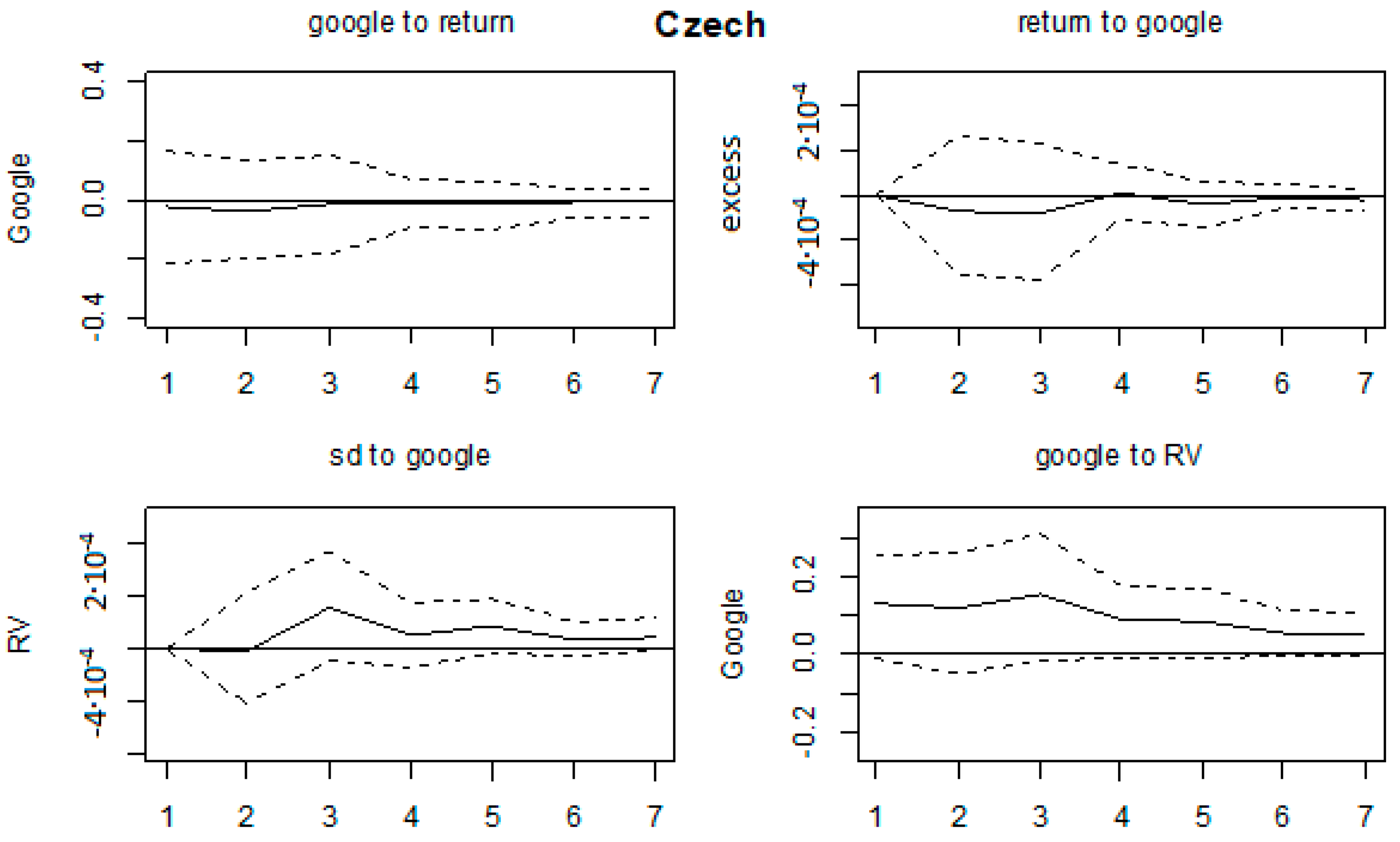
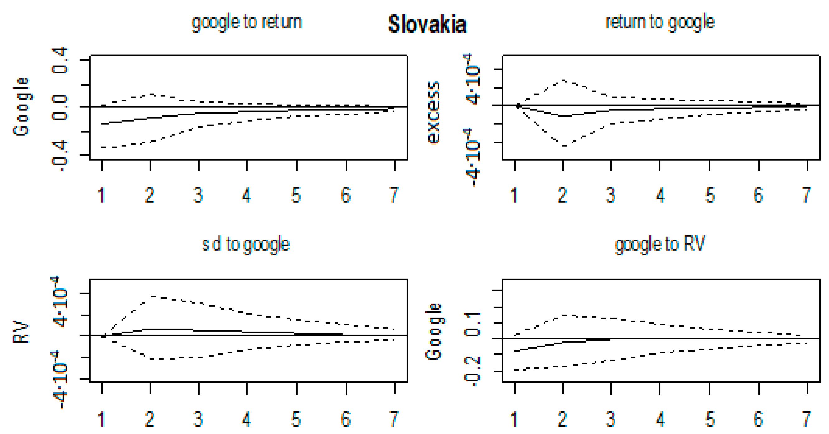
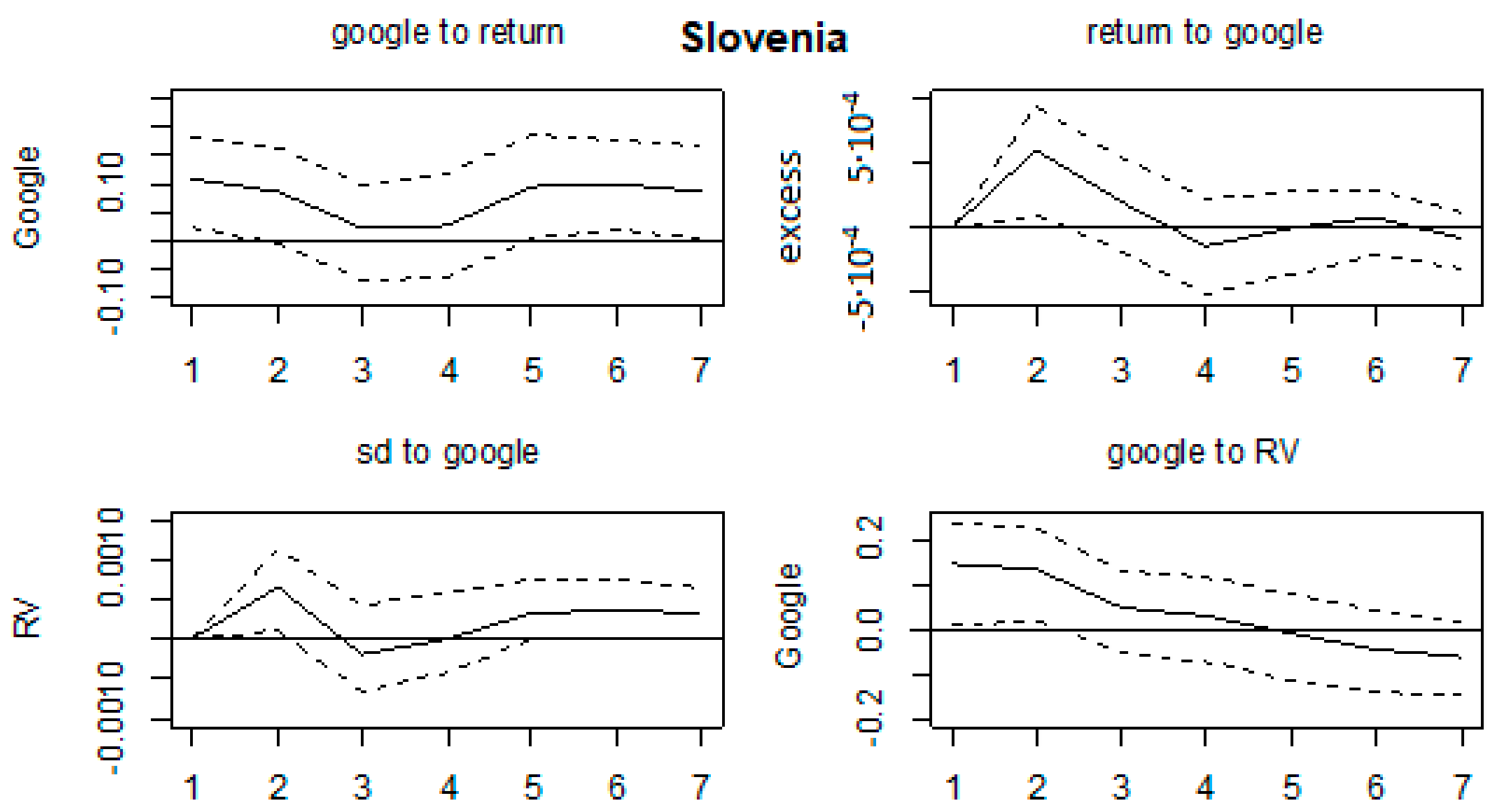
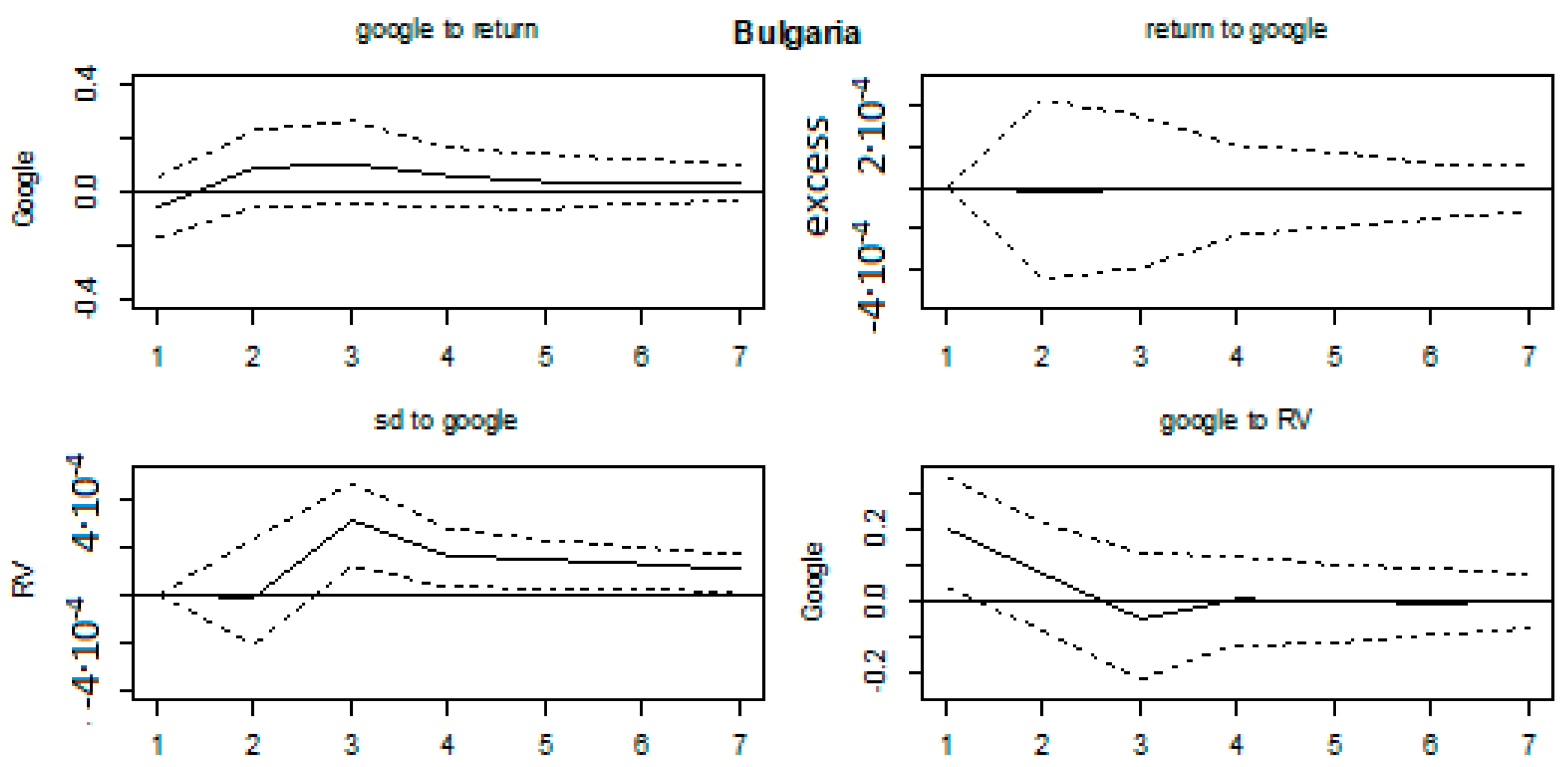
From the website Investing (2019) we obtained the daily data on stock indices for the following countries: Hungary, Croatia, Slovenia, Slovakia, Serbia, Bosnia and Herzegovina, Bulgaria, Ukraine, Poland and the Czech Republic. Main indices of each country were used for the rest of the study (names are given in Table 1, which are the search terms within Google trends data as well, in the category of finance). Names of indices were used as search terms, due to observing national indices in the study, as previous research has this approach as well: Hamid and Heiden (2015) use term “dow” for the DOW index; “dow”, “S&P 500” and “NASDAQ” were used for the same indices in Vozlyublennaia (2014); “crobex” for CROBEX in Škrinjarić (2018a); “dax” for DAX in Škrinjarić and Čižmešija (2019); terms regarding names of following markets in Padungsaksawasdi et al. (2019): Chinese, Indian, Malaysian, Thailand, Australian, Hong Kong, Japanese, Korean, New Zealand and Singaporean; and 67 country index names in Chen (2017), etc.4. Since we used the names of the indices, this means that we were observing noise-traders (or retail investors), due to explanations given in Peng and Xiong (2006), Da et al. (2011), Odean (1998), Grinblatt and Keloharju (2000), Black (1986) and De Long et al. (1990): Retail investors are more likely to use Internet searches for the comparisons of investment opportunities, due to not being able to process as much information as professional investors do. Thus, noise investors opt to focus on broader indices compared to specific stocks. That is why some models (Black 1986; De Long et al. 1990) forecast that such behavior from noise traders leads to increases of volatility.
Based on daily values, the daily return series were calculated and were then converted to a monthly basis by calculating monthly average returns. Moreover, for the risk series we calculated the realized volatility, by following Andersen and Bollerslev (1998) and Barndorff-Nielsen and Shepard (2002): R V τ = t = 1 τ r t 2 , where rt is the daily return series within a month. Finally, for the variable of investor’s attention, we used the standardized values of Google Trends Data (2019) on the search volume for every index name in each country. The search engine Google was used due to it representing the greatest majority of the online search volume (see Netmarketshare 2019; over 75% since 2016). Detailed reasoning can be found in Da et al. (2011), such as it being an exact query, the search volume on Google is becoming larger every day and can capture sentiment, i.e., attention of both individual and institutional investors, especially individual ones (Peng and Xiong 2006). The search volume from Google trends data is a relative measure, ranging from 0 to 100, due to its representing total searches of the geography and time range so that the popularity of an expression is expressed relatively. The reasoning why we calculated monthly return and volatility series is that Google trends data for the observed countries was available only on a monthly basis, i.e., the search terms regarding names of the stock market indices within the finance category of Google trends data were available on a monthly basis. Index name (last column of Table 1) was used as a search term. Time span for every country differs, which can be seen in Table 1. Most data was available for Croatia and Ukraine and least amount for Bosnia and Herzegovina and Serbia (N column).
Before the analysis, all of the variables were tested for unit roots, with detailed results shown in Appendix A in Table A1. All of the variables were found to be stationary, thus we proceeded with VAR modeling. Moreover, Figure A1, Figure A2, Figure A3, Figure A4, Figure A5, Figure A6, Figure A7, Figure A8, Figure A9 and Figure A10 depict monthly time series of excess return, realized volatility and Google search volume (GSV from now on) for every country.

4.2. VAR Results

The adequate lag length for VAR models was checked by calculating the usual information criteria. Then, the model was estimated by going from the smallest number of lag until there was no problem of multivariate autocorrelation and heteroskedasticity found. Optimal lag lengths are shown in Table 2. Detailed results on mentioned tests of autocorrelation and heteroskedasticity for lag lengths in Table 2 are shown in Appendix A in Table A2. Thus, the rest of the analysis was continued with lag lengths from Table 2.
Granger causality tests have been conducted in every VAR model. Results are given in Table 3. Here, each value by column depicts the partial F test value for the null hypothesis that the series in that column does not Granger cause the other two series in the VAR model. It could be seen that the GSV variable Granger causes the other two variables for only the Hungarian, Croatian, Ukrainian, Serbian and Slovenian markets. This indicates that the investor’s attention variable could affect return and volatility series on the mentioned markets to some extent. Interesting results are in the column denoted RV, where it was seen that the variable RV Granger causes the other two variables. Finally, the excess return Granger causes the other two variables only on the Croatian, Hungarian and Slovenian markets. The Bosnian market was the only one with significant results regarding excess return causing other variables in the model (on 10%). The other markets seemed not to be having causal effects between any of the variables. The reason for such results could be in the small sample size due to unavailability of data. However, since the Granger test did not indicate the sign of the found effects in each variable, we continued to the impulse response functions.
All of the impulse response functions were graphed in Figure A11, Figure A12, Figure A13, Figure A14, Figure A15, Figure A16, Figure A17, Figure A18, Figure A19 and Figure A20 in Appendix A, with confidence intervals being constructed by bootstrapping them with 1000 replications. We could comment on the relevant results. Firstly, no effects on any of the variables were found for the Ukrainian, Bosnian, Czech and Slovakian markets. This was in line with the results in Table 3. Next, the majority of the significant results were found for Hungarian, Croatian, Slovenian and Polish markets. On the Hungarian market, RV shocks affected GSV series in the first three months, by increasing the search volume. Shocks in GSV negatively affected the return series at lags 3 and 5. Next, on the Croatian market, shocks in GSV caused a decrease of return series in the first two months and a RV increase in the first two months as well. Shocks in the volatility series led to an increase of GSV in the first month. The Polish market was characterized by an increase of GSV in the first 2 months as a result of shocks in RV. On the Slovenian market, the results indicate that shocks in return series led to an increase of GSV in months 1 and 6. The return series were increased in the first 2 months as a result of shocks in GSV, whereas the RV series also rose in the first 2 months after a GSV shock. Moreover, GSV increased in the first 2 months as a result of shocks in RV. Some marginal results were found on the Polish market (shocks in RV led to an increase of GSV until the second month); Serbian (RV increased in first 2 months as a result of a shock in GSV) and Bulgarian (lagged effects of shocks in GSV on RV series, from third month onwards).
The results in which shocks in GSV led to negative values of return series was in line with Dimpfl and Jank (2016); as well as the increase of GSV caused by shocks in volatility series being in line with Vozlyublennaia (2014). By comparing the mentioned results, it could be said that the investor’s attention hypothesis could be confirmed only on the Hungarian and Croatian markets. Other markets did not experience such predictability. The results for other markets are in line with Chen et al. (2002) where a positive relationship was found between stock return and investor recognition (breadth of ownership). Thus, mixed results were found here, as in the previous literature, which could be explained by differences in the (tax related) legislation, depth of the markets, macroeconomic fundamentals, financial exposure, etc. This was in line with explanations given in Sibley et al. (2016), where the investor sentiment variable was strongly related to economic fundamentals, which in turn are important in asset pricing models.

4.3. Spillover Indices Results

Next, we moved forward to the estimation of the total spillovers within every VAR model for the entire sample. Table 4, Table 5, Table 6, Table 7, Table 8, Table 9, Table 10, Table 11, Table 12 and Table 13 depict the total spillover indices (bolded values in the bottom left corner) and all of the directional indices, based on the forecast horizon h = 12 (as in Antonakakis et al. 2016). E.g., by focusing on Table 4, the total variability of return series on the Serbian market was explained by shocks in the return series in the amount of 95.34%; by shocks in RV in the amount of 2.30% and GSV 2.36%. Total spillover in the observed period between all of the variables was small and was equal to 6.42%. Similar interpretations could be made for every other following table. The smallest spillovers were found for the aforementioned Serbian market, as well as Bosnian, Ukrainian, Czech, Bulgarian and Slovakian markets. The greatest spillovers were found on the Hungarian, Croatian, Slovenian and Polish markets. These tables are useful for (potential) investors in order to estimate the amount of volatility of a variable caused by other variables in the system and to which extent the lead values of some variables can cause future values of other variables. If one focuses on the columns labeled GSV, it can be seen that the shocks in Google search volume explain a greater percentage of risk series (RV) when compared to return series in the majority of cases. This is especially true for the markets where the greatest total spillovers are found. This result is in line with Andrei and Hasler (2014) and Vlastakis and Markellos (2012), where greater volatility predictability over return predictability is found by using GSV.
In order to account for the dynamics over time, we calculated rolling spillover indices, with a 30 month rolling window length (as in Antonakakis et al. 2016). Thus, the dynamics could be commented on. The rolling spillover indices are shown in Figure 1 and Figure 2. This could help to forecast when the spillovers between variables in the model would increase or decrease in order to tailor specific international portfolio strategies. When an investor expects an increase of total spillover between the return, volatility and search volume variables, he can better forecast all of the variables and thus either buy or sell on individual markets, depending on forecasts and investor’s preferences. The greatest spillovers over time were found for the Hungarian, Croatian, Slovenian and Ukrainian markets. Thus, these markets had the potential to violate the EMH. This is in line with Andries et al. (2018) and Škrinjarić (2018c), and the lack of spillovers for the Polish market is in line with Ferreira (2018).
Moreover, detailed insights are provided on Figure 3, Figure 4, Figure 5, Figure 6, Figure 7, Figure 8, Figure 9, Figure 10, Figure 11 and Figure 12, where the net indices for every variable are shown. Now, an investor could obtain information on which variable gives shocks to others in the system, and in which period. This contributes to the literature by looking at which variable is the net emitter of shocks in different market conditions. Positive values of each index indicate that that variable was the net emitter of shocks. Net values were smaller for those countries in which the total spillover index was smaller as well, and the opposite was true for those countries with greater spillover values in Table 4, Table 5, Table 6, Table 7, Table 8, Table 9, Table 10, Table 11 and Table 12. In the Hungarian case, the RV and GSV variables were, for the majority of the time, net givers of shocks. In Croatia, the financial crisis of 2008 shows that the GSV was the net emitter of shocks (similar was true for 2017, when a local crisis caused by the Agrokor concern was happening, for details please see Škrinjarić (2018b) and Škrinjarić and Orlović (2019)). In the rest of the observed period, there was an interchangeability of net emitters and receivers of shocks. On the Ukrainian market, the RV variable was the net emitter of shocks in the last 3 years; Serbian market was characterized by the GSV being the net emitter most of the time and this was true for the variable RV in the middle of the observed period on the Bosnian market. All three variables were sometimes receivers and sometimes emitters of shocks on the Slovakian and Slovenian markets, with GSV being the net receiver on the Bulgarian market. Finally, the GSV was the net giver of shocks in almost the entire observed period on the Polish market.
These findings indicate that some dynamics should be observed in such modeling. The differences of increasing and decreasing spillovers over time between markets, of course, exist. These could be due to political, economic, social and other intra-country events, which are specific to that country alone. However, the results that were found to be significant could be explained by non-efficiencies of the observed markets, which is in line with Necula and Radu (2012)5 and Baele et al. (2015)6.

5. Conclusions

Summarizing the previous results, several things could be said. The results somewhat indicated that some of the stock markets exhibited violation of the EMH to some extent. This included the Hungarian, Slovenian and Croatian markets, while some weaker evidence was found for the Bulgarian and Polish markets. This was based on the results of Granger causality tests and the spillover tables’ results. The impulse response functions gave insights into (non) rejection of investor’s attention hypothesis. Namely, the Hungarian, Polish, Slovenian and Croatian markets were found to have the majority of significant results here. An increase in the variable Google search volume led to a decrease of return series on the Croatian and Hungarian markets, which was in favor of Merton’s (1987) theoretical findings. Moreover, sometimes the risk variable reacted even more to shocks in the search volume variable, which was in accordance with Andrei and Hasler (2014) and Vlastakis and Markellos (2012).
Violating the efficient market hypothesis in terms of investor’s attention towards specific groups of stocks is getting more focus in research over the last couple of years. The empirical literature on testing the predictability of stock returns and volatilities by including the online search volume in existing models has been booming, especially in the last decade. This paper wanted to get initial insights into the relationship between the Google search volumes and risk and return series for selected CEE and SEE stock markets. Reasoning lies upon the facts that such markets are rarely observed in similar studies and getting more information on these markets can be useful for (potential) investors.
With the main results being mixed, depending on the observed market, recommendations for international investors have to be based on the findings for individual markets. For those markets in which we found predictability of selected variables to some extent, investors could utilize these results for future forecasting. This could enhance portfolio performance in terms of risk and return. Some shortfalls should be mentioned as well. Data unavailability on some indices did not enable a long-term analysis for some of the countries in the sample. Thus, the results could very well be influenced by it. With that in mind, future work should repeat this analysis in order to test the validity of results given here.
Contributions of the research are found in extending the VAR framework with spillover indices: Total and directional, both static and dynamic. The time varying shocks spillover enabled us to provide comments on the dynamics between the selected variables. Moreover, the dynamic net spillover indices were estimated, so the information on which variable is the net emitter or net receiver of shocks in the system was obtained as well. Future work should focus on individual countries in order to get detailed insights in the dynamics of risks, returns and search volumes specific to a given country. In that way, with detailed results we will be able to simulate and compare investment strategies tailored on individual specific results.

Funding

This research received no external funding. The APC was funded by institutions through the Knowledge Unlatched initiative and partially funded by MDPI.

Acknowledgments

The author would like to thank the two referees for useful comments that have contributed to the final quality of the paper.

Conflicts of Interest

The author declares no conflict of interest.

Appendix A

Table A1. Unit root test results for variables, constant included.
CountryReturnExcess ReturnRealized VolatilityGoogle Search Volume
Hungary−7.0149 ***−5.789 ***−4.2054 ***−3.6045 ***
Croatia−8.2586 ***−9.922 ***−6.4532 ***−3.1011 **
Ukraine−9.077 ***−9.500 ***−7.123 ***−4.1481 ***
Slovenia−6.0497 ***−9.233 ***−6.1911 ***−2.8907 **
Poland−7.3147 ***−7.483 ***−5.3317 ***−4.5645 ***
Bosnia and Herzegovina−5.4507 ***−6.227 ***−4.7188 ***−5.3291 ***
Czech Republic−8.8916 ***−8.778 ***−5.9225 ***−3.633 ***
Slovakia−7.1175 ***−6.902 ***−5.5583 ***−4.295 ***
Bulgaria−5.5037 ***−6.945 ***−6.279 ***−2.6779 *
Serbia−6.9199 ***−6.622 ***−5.4058 ***−3.7528 ***
Note: Results in Table A1 show empirical test values, where *, ** and *** denote statistical significance on 10%, 5% and 1% respectively. Constant is included in the ADF test as a deterministic regressor.
Table A2. Multivariate autocorrelation and heteroskedasticity tests.
CountryMultivariate Test
ARCH TestLM Test
Hungary413.320 (0.733)47.697 (0.092) *
Croatia400.230 (0.302)13.901 (0.126)
Ukraine14.959 (0.092) *38.405 (0.361)
Slovenia48.593 (0.078) *26.446 (0.090) *
Poland437.540 (0.417)99.827 (0.700)
Bosnia and Herzegovina396.000 (0.892)18.77 (0.406)
Czech Republic443.040 (0.346)10.973 (0.278)
Slovakia453.760 (0.226)119.68 (0.208)
Bulgaria438.880 (0.412)131.48 (0.062) *
Serbia396.000 (0.892)99.431 (0.710)
Note: * denotes statistical significance on 10%. Test results are provided for the 12th order autocorrelation and heteroskedasticity. Table shows empirical test values for each test and each country with p-values given in brackets.
Figure A1. Comparison of monthly series: Excess return, RV and Google search volume, Serbia.
Ijfs 07 00059 g0a1
Figure A2. Comparison of monthly series: Excess return, RV and Google search volume, Hungary.
Ijfs 07 00059 g0a2
Figure A3. Comparison of monthly series: Excess return, RV and Google search volume, Croatia.
Ijfs 07 00059 g0a3
Figure A4. Comparison of monthly series: Excess return, RV and Google search volume, Ukraine.
Ijfs 07 00059 g0a4
Figure A5. Comparison of monthly series: Excess return, RV and Google search volume, Bosnia and Herzegovina.
Ijfs 07 00059 g0a5
Figure A6. Comparison of monthly series: Excess return, RV and Google search volume, Czech Republic.
Ijfs 07 00059 g0a6
Figure A7. Comparison of monthly series: Excess return, RV and Google search volume, Slovakia.
Ijfs 07 00059 g0a7
Figure A8. Comparison of monthly series: Excess return, RV and Google search volume, Slovenia.
Ijfs 07 00059 g0a8
Figure A9. Comparison of monthly series: Excess return, RV and Google search volume, Bulgaria.
Ijfs 07 00059 g0a9
Figure A10. Comparison of monthly series: Excess return, RV and Google search volume, Poland.
Ijfs 07 00059 g0a10
Figure A11. Impulse response functions, Serbia.
Ijfs 07 00059 g0a11
Figure A12. Impulse response functions, Hungary.
Ijfs 07 00059 g0a12
Figure A13. Impulse response functions, Croatia.
Ijfs 07 00059 g0a13
Figure A14. Impulse response functions, Ukraine.
Ijfs 07 00059 g0a14
Figure A15. Impulse response functions, Bosnia and Herzegovina.
Ijfs 07 00059 g0a15
Figure A16. Impulse response functions, Czech Republic.
Ijfs 07 00059 g0a16
Figure A17. Impulse response functions, Slovakia.
Ijfs 07 00059 g0a17
Figure A18. Impulse response functions, Slovenia.
Ijfs 07 00059 g0a18
Figure A19. Impulse response functions, Bulgaria.
Ijfs 07 00059 g0a19
Figure A20. Impulse response functions, Poland.
Ijfs 07 00059 g0a20

References

  1. Aalborg, Halvor Aarhus, Peter Molnár, and Jon Erik de Vries. 2019. What can explain the price, volatility and trading volume of Bitcoin? Finance Research Letters 29: 255–65. [Google Scholar] [CrossRef]
  2. Andersen, Torben, and Tim Bollerslev. 1998. Answering the sceptics: Yes standard volatility models do provide accurate forecasts. International Economic Review 39: 885–905. [Google Scholar] [CrossRef]
  3. Andrei, Daniel, and Michael Hasler. 2014. Investor attention and stock market volatility. The Review of Financial Studies 28: 33–72. [Google Scholar] [CrossRef]
  4. Andries, Alin Marius, Iulian Ihnatov, and Nicu Sprincean. 2018. Do seasonal anomalies still exist in central and eastern European countries? A conditional variance approach. Romanian Journal of Economic Forecasting 20: 60–83. [Google Scholar]
  5. Antonakakais, Nikolas, Cristhophe Andre, and Rangan Gupta. 2016. Dynamic Spillovers in the United States: Stock Market, Housing, Uncertainty, and the Macroeconomy. Southern Economic Journal 83: 609–24. [Google Scholar] [CrossRef]
  6. Baele, Lieven, Geert Bekaert, and Larissa Schäfer. 2015. An Anatomy of Central and Eastern European Equity Markets. Columbia Business School Working Paper, No. 15–71. Singapore: Columbia Business School. [Google Scholar]
  7. Bank, Matthias, Martin Larch, and Georg Peter. 2011. Google search volume and its influence on liquidity and returns of German stocks. Financial Markets and Portfolio Management 25: 239–64. [Google Scholar] [CrossRef]
  8. Barber, Brad, and Terrance Odean. 2007. All that glitters: The effect of attention and news on the buying behavior of individual and institutional investors. Review of Financial Studies 21: 785–818. [Google Scholar] [CrossRef]
  9. Barndorff-Nielsen, Ole, and Neil Shephard. 2002. Econometric analysis of realised volatility and its use in estimating stochastic volatility models. Journal of the Royal Statistical Society 64: 253–80. [Google Scholar] [CrossRef]
  10. Bijl, Laurens, Glenn Kringhaug, Peter Molnár, and Eirik Sandvik. 2016. Google searches and stock returns. International Review of Financial Analysis 45: 150–56. [Google Scholar] [CrossRef]
  11. Black, Fischer. 1986. Noise. The Journal of Finance 41: 529–43. [Google Scholar] [CrossRef]
  12. Bortoli, Clement, and Stephane Combes. 2015. Contribution from Google Trends for Forecasting the Short-Term Economic Outlook in France: Limited Avenues. Institut National de la Statistique et des Éstudes Économiques. Available online: https://www.insee.fr/en/statistiques/1408911?sommaire=1408916 (accessed on 25 May 2019).
  13. Chen, Tao. 2017. Investor Attention and Global Stock Returns. Journal of Behavioral Finance 18: 358–72. [Google Scholar] [CrossRef]
  14. Chen, Joseph, Harrison Hong, and Jeremy Stein. 2002. Breadth of Ownership and Stock Returns. Journal of Financial Economics 66: 171–205. [Google Scholar] [CrossRef]
  15. Chen, Jian, Guohao Tang, Jiaquan Yao, and Guofu Zhou. 2019. Investor Attention and Stock Returns. Available online: https://ssrn.com/abstract=3194387 (accessed on 25 May 2019).
  16. Da, Zhi, Joseph Engelberg, and Pngjie Gao. 2010. The Sum of All Fears: Investor Sentiment and Asset Prices, SSRN eLibrary. Available online: https://pdfs.semanticscholar.org/cc4f/6f4dba88381810412ea3d929715f38cb9ee0.pdf (accessed on 25 May 2019).
  17. Da, Zhi, Joseph Engelberg, and Pengjie Gao. 2011. In search of attention. The Journal of Finance 66: 1461–99. [Google Scholar] [CrossRef]
  18. De Long Bradford, James, Andrei Shleifer, Lawrence Summers, and Robert Waldmann. 1990. Noise trader risk in financial markets. Journal of Political Economy 98: 703–38. [Google Scholar] [CrossRef]
  19. Demirer, Mert, Umut Gokcen, and Kamil Yilmaz. 2018. Financial Sector Volatility Connectedness and Equity Returns. Koc University-TUSIAD Economic Research Forum, Working Paper No. 1803. Istanbul: Koc University. [Google Scholar]
  20. Dergiades, Theologos, Eleni Mavragani, and Bing Pan. 2018. Google trends and tourists’ arrivals: Emerging biases and proposed corrections. Tourism Management 66: 108–20. [Google Scholar] [CrossRef]
  21. Diebold, Francis, and Kamil Yilmaz. 2009. Measuring Financial Asset Return and Volatility Spillovers with Application to Global Equity Markets. The Economic Journal 119: 158–71. [Google Scholar] [CrossRef]
  22. Diebold, Francis, and Kamil Yilmaz. 2011. Equity Market Spillovers in the Americas. In Financial Stability, Monetary Policy, and Central Banking. Bank of Chile Central Banking Series 5; Edited by Rodrigo Alfaro. Santiago: Bank of Chile Central Banking, pp. 199–214. [Google Scholar]
  23. Diebold, Francis, and Kamil Yilmaz. 2012. Better to Give than to Receive: Predictive Directional Measurement of Volatility Spillovers. International Journal of Forecasting 28: 57–66. [Google Scholar] [CrossRef]
  24. Dimpfl, Thomas, and Stephan Jank. 2016. Can Internet Search Queries Help to Predict Stock Market Volatility? European Financial Management 22: 171–92. [Google Scholar] [CrossRef]
  25. Dzielinski, Michal. 2012. Measuring economic uncertainty and its impact on the stock market. Finance Research Letters 9: 167–75. [Google Scholar] [CrossRef]
  26. Fama, Eugene. 1965. Random Walks in Stock Market Prices. Financial Analysts Journal 21: 55–59. [Google Scholar] [CrossRef] [Green Version]
  27. Fama, Eugene. 1970. Efficient Capital Markets: A Review of Theory and Empirical Work. The Journal of Finance 25: 383–417. [Google Scholar] [CrossRef]
  28. Fang, Lily, and Joel Peress. 2009. Media Coverage and the Cross-section of Stock Returns. The Journal of Finance 64: 2023–52. [Google Scholar] [CrossRef]
  29. Ferreira, Paulo. 2018. Long-range dependencies of Eastern European stock markets: A dynamic detrended analysis. Physica A 505: 454–70. [Google Scholar] [CrossRef]
  30. Frieder, Laura, and Avanidhar Subrahmanyam. 2005. Brand Perceptions and the Market for Common Stock. Journal of Financial and Quantitative Analysis 40: 57–85. [Google Scholar] [CrossRef]
  31. Goddard, John, Arben Kita, and Qingwei Wang. 2015. Investor attention and FX market volatility. Journal of International Financial Markets, Institutions & Money 38: 79–96. [Google Scholar] [Green Version]
  32. Goel, Sharad, Jake Hofman, Sebastien Lahaie, David Pennock, and Duncan Watts. 2010. Predicting consumer behavior with Web search. Proceedings of the National Academy of Sciences of the United States of America 107: 17486–90. [Google Scholar] [CrossRef]
  33. Google Trends Data. 2019. Available online: https://trends.google.com/trends/ (accessed on 25 May 2019).
  34. Grinblatt, Mark, and Matti Keloharju. 2000. The investment behavior and performance of various investor types: A study of Finland’s unique data set. Journal of Financial Economics 55: 43–67. [Google Scholar] [CrossRef]
  35. Grullon, Gustavo, George Kanatas, and James Weston. 2004. Advertising, breadth of ownership, and liquidity. Review of Financial Studies 17: 439–61. [Google Scholar] [CrossRef]
  36. Habibah, Ume, Suresh Rajput, and Ranjeta Sadhwani. 2017. Stock market return predictability: Google pessimistic sentiments versus fear gauge. Cogent Economics & Finance 5: 1390897. [Google Scholar]
  37. Hamid, Alain, and Moritz Heiden. 2015. Forecasting volatility with empirical similarity and Google Trends. Journal of Economic Behavior & Organization 117: 62–81. [Google Scholar]
  38. Han, Liyan, Ziying Li, and Libo Yin. 2017. Investor Attention and Stock Returns: International Evidence. Emerging Markets Finance and Trade 54: 3168–88. [Google Scholar] [CrossRef]
  39. Havranek, Tomas, and Ayaz Zeynalov. 2018. Forecasting Tourist Arrivals: Google Trends Meets Mixed Frequency Data. Munich Personal RePEc Archive, MPRA paper No. 90203. Munich: Munich University Library. [Google Scholar]
  40. Investing Data Website. 2019. Available online: https://www.investing.com/ (accessed on 25 May 2019).
  41. Joseph, Kissain, Babajide Wintoki, and Zelin Zhang. 2011. Forecasting abnormal stock returns and trading volume using investor sentiment: Evidence from online search. International Journal of Forecasting 27: 1116–27. [Google Scholar] [CrossRef]
  42. Jun, Seung-Pyo, Hyoung Sun Yoo, and San Choi. 2018. Ten years of research change using Google Trends: From the perspective of big data utilizations and applications. Technological Forecasting & Social Change 130: 69–87. [Google Scholar]
  43. Khan, Mehwish Aziz, and Eatzaz Ahmad. 2018. Measurement of Investor Sentiment and Its Bi-Directional Contemporaneous and Lead–Lag Relationship with Returns: Evidence from Pakistan. Sustainability 11: 94. [Google Scholar] [CrossRef]
  44. Kim, Neri, Katarína Lučivjanská, Peter Molnár, and Roviel Villa. 2019. Google searches and stock market activity: Evidence from Norway. Finance Research Letters 28: 208–20. [Google Scholar] [CrossRef]
  45. Koop, Gary, Mashem Pesaran, and Simon Potter. 1996. Impulse response analysis in nonlinear multivariate models. Journal of Econometrics 74: 119–47. [Google Scholar] [CrossRef]
  46. Lehavy, Reuven, and Richard Sloan. 2008. Investor recognition and stock returns. Review of Accounting Studies 13: 327–61. [Google Scholar] [CrossRef]
  47. Li, Jun, and Jiangfeng Yu. 2012. Investor Attention, Psychological Anchors, and Stock Return Predictability. Journal of Financial Economics 104: 401–19. [Google Scholar] [CrossRef]
  48. Lütkepohl, Helmut. 1993. Introduction to Multiple Time Series Analysis. Berlin: Springer. [Google Scholar]
  49. Lütkepohl, Helmut. 2006. New Introduction to Multiple Time Series Analysis. Berlin: Springer. [Google Scholar]
  50. Lütkepohl, Helmut. 2010. Vector Autoregressive Models. Economics Working Paper ECO 2011/30. Fiesole: European University Institute. [Google Scholar]
  51. Merton, Robert. 1987. A simple model of capital market equilibrium with incomplete information. The Journal of Finance 42: 483–510. [Google Scholar] [CrossRef]
  52. Molnár, Peter, and Milan Bašta. 2017. Google searches and Gasoline prices. Paper presented at 2017 14th International Conference on the European Energy Market (EEM), Dresden, Germany, June 6–9; pp. 1–5. [Google Scholar]
  53. Mondria, Jordi, Thomas Wu, and Yi Zhang. 2010. The determinants of international investment and attention allocation: Using internet search query data. Journal of International Economics 82: 85–95. [Google Scholar] [CrossRef] [Green Version]
  54. Necula, Ciprian, and Alina-Nicoleta Radu. 2012. Long Memory in Eastern European Financial Markets Returns. Economic Research 25: 316–77. [Google Scholar] [CrossRef]
  55. Netmarketshare. 2019. Available online: https://netmarketshare.com (accessed on 25 May 2019).
  56. Odean, Terrance. 1998. Are investors reluctant to realize their losses? The Journal of Finance 53: 1775–98. [Google Scholar] [CrossRef]
  57. Önder, Irem. 2017. Forecasting tourism demand with Google trends: Accuracy comparison of countries versus cities. International Journal of Tourism Research 19: 648–660. [Google Scholar] [CrossRef]
  58. Padungsaksawasdi, Chaiyuth, Sirimon Treepongkaruna, and Robert Brooks. 2019. Investor Attention and Stock Market Activities: New Evidence from Panel Data. International Journal of Financial Studies 7: 30. [Google Scholar] [CrossRef]
  59. Peng, Lin, and Wei Xiong. 2006. Investor attention, overconfidence and category learning. Journal of Financial Economics 80: 563–602. [Google Scholar] [CrossRef] [Green Version]
  60. Pesaran, Hashem, and Yongcheol Shin. 1998. Generalized impulse response analysis in linear multivariate models. Economics Letters 58: 17–29. [Google Scholar] [CrossRef]
  61. Preis, Tobias, Daniel Reith, and Eugene Stanley. 2010. Complex dynamics of our economic life on different scales: Insights from search engine query data. Philosophical Transactions of the Royal Society A 368: 5707–19. [Google Scholar] [CrossRef]
  62. Preis, Tobias, Helen Susannah Moat, and Eugene Stanley. 2013. Quantifying Trading Behavior in Financial Markets Using Google Trends. Scientific Reports 3: 1684. [Google Scholar] [CrossRef]
  63. Sibley, Steven, Yanchu Wang, Yuhang Xing, and Xiaoyan Zhang. 2016. The information content of the sentiment index. Journal of Banking & Finance 62: 164–79. [Google Scholar]
  64. Škrinjarić, Tihana. 2018a. Mogu li Google trend podaci poboljšati prognoziranje prinosa na Zagrebačkoj burzi? (Can Google trend data enhance return forecasting on Zagreb Stock Exchange?). Zbornik radova Ekonomskog fakulteta Sveučilišta u Mostaru (Journal of Economy and Business, University of Mostar) 24: 58–76. [Google Scholar]
  65. Škrinjarić, Tihana. 2018b. The value of food sector on Croatian capital market if the Agrokor crisis did not happen: Synthetic control method approach. CEA Journal of Economics 13: 53–65. [Google Scholar]
  66. Škrinjarić, Tihana. 2018c. Testing for Seasonal Affective Disorder on Selected CEE and SEE Stock Markets. Risks 6: 140. [Google Scholar] [CrossRef]
  67. Škrinjarić, Tihana, and Mirjana Čižmešija. 2019. Investor attention and risk predictability: A spillover index approach. Paper presented at the 15th International Symposium on Operations Research in Slovenia, Bled, Slovenia, September 25–27; pp. 423–28. [Google Scholar]
  68. Škrinjarić, Tihana, and Zrinka Orlović. 2019. Effects of economic and political events on stock returns: Event study of Agrokor case in Croatia. Croatian Economic Survey 21: 47–86. [Google Scholar] [CrossRef]
  69. Smith, Geoffrey Peter. 2012. Google Internet Search Activity and Volatility Prediction in the Market for Foreign Currency. Finance Research Letters 9: 103–10. [Google Scholar] [CrossRef]
  70. Takeda, Fumika, and Takumi Wakao. 2014. Google search intensity and its relationship with returns and trading volume of Japanese stocks. Pacific-Basin Finance Journal 27: 1–18. [Google Scholar] [CrossRef]
  71. Tan, Selin Düz, and Oktay Tas. 2019. Investor attention and stock returns: Evidence from Borsa Istanbul. Borsa Istanbul Review 19: 106–16. [Google Scholar]
  72. Tantaopas, Parkpoom, Chaiyuth Padungsaksawasdi, and Sirimon Treepongkaruna. 2016. Attention effect via internet search intensity in Asia-Pacific stock markets. Pacific-Basin Finance Journal 38: 107–24. [Google Scholar] [CrossRef]
  73. Tkacz, Greg. 2013. Predicting Recessions in Real-Time: Mining Google Trends and Electronic Payments Data for Clues. C.D. Howe Institute, Issue 387. Toronto: C. D. Howe Institute Commentary. [Google Scholar]
  74. Urbina, Jilber. 2013. Financial Spillovers across Countries: Measuring Shock Transmissions. MPRA Working Paper. Munich: Munich Personal RePEc Archive. [Google Scholar]
  75. Vlastakis, Nikolas, and Raphael Markellos. 2012. Information demand and stock market volatility. Journal of Banking & Finance 36: 1808–21. [Google Scholar]
  76. Vosen, Simeon, and Torsten Schmidt. 2011. Forecasting Private Consumption: Survey Based Indicators vs. Google Trends. Journal of Forecasting 30: 565–78. [Google Scholar] [CrossRef]
  77. Vozlyublennaia, Nadia. 2014. Investor attention, index performance, and return predictability. Journal of Banking & Finance 41: 17–35. [Google Scholar]
  78. Woo, Jaemin, and Ann Owen. 2019. Forecasting private consumption with Google Trends data. Journal of Forecasting 38: 81–89. [Google Scholar] [CrossRef]
  79. Yang, Tian, Jinsong Liu, Qianwei Ying, and Tahir Yousaf. 2019. Media Coverage and Sustainable Stock Returns: Evidence from China. Sustainability 11: 2335. [Google Scholar] [CrossRef]
  80. Zhang Wei, Dehua Shen, Yongjie Zhang, and Xiong Xiong. 2013. Open source information, investor attention, and asset pricing. Economic Modelling 33: 613–619. [Google Scholar] [CrossRef]
  81. Zhang, Junru, Hadrian Geri Djajadikerta, and Zhaoyong Zhang. 2018. Does Sustainability Engagement Affect Stock Return Volatility? Evidence from the Chinese Financial Market. Sustainability 10: 3361. [Google Scholar] [CrossRef]
1
For details, please see Lehavy and Sloan (2008).
2
Autoregressive integrated moving average—generalized autoregressive conditional heteroskedasticity.
3
Vector auto regression.
4
Individual company names are utilized in studies, which observe those company returns series, as in Preis et al. (2010); Bijl et al. (2016); Tan and Tas (2019) and Khan and Ahmad (2018).
5
Authors observed Romania, Hungary, Czech Republic, Poland, Slovenia, Bulgaria, Slovakia and Croatia and found inefficiencies of the stock markets by using the fractional differencing approach.
6
Authors compared CEE stock markets by using a variety of measures regarding growth, development, concentration, etc. Although these countries faced a similar past regarding the economic system, their stock markets today have somewhat great differences in terms of market concentration, liquidity, etc.
Figure 1. Total spillover indices (from top to bottom, left to right): Serbia, Hungary, Croatia, Ukraine, Bosnia and Herzegovina and Czech Republic.
Ijfs 07 00059 g001
Figure 2. Total spillover indices (from top to bottom, left to right): Slovakia, Slovenia, Bulgaria and Poland.
Ijfs 07 00059 g002
Figure 3. Net rolling indices, Hungary.
Ijfs 07 00059 g003
Figure 4. Net rolling indices, Croatia.
Ijfs 07 00059 g004
Figure 5. Net rolling indices, Ukraine.
Ijfs 07 00059 g005
Figure 6. Net rolling indices, Serbia.
Ijfs 07 00059 g006
Figure 7. Net rolling indices, Bosnia and Herzegovina.
Ijfs 07 00059 g007
Figure 8. Net rolling indices, Slovakia.
Ijfs 07 00059 g008
Figure 9. Net rolling indices, Slovenia.
Ijfs 07 00059 g009
Figure 10. Net rolling indices, Bulgaria.
Ijfs 07 00059 g010
Figure 11. Net rolling indices, Poland.
Ijfs 07 00059 g011
Figure 12. Net rolling indices, the Czech Republic.
Ijfs 07 00059 g012
Table 1. Data time span by country.
CountryInitial DateNIndex Name
HungaryMarch 2011100BUX
CroatiaJanuary 2004186CROBEX
UkraineJanuary 2004186PFTS
SloveniaApril 2006159SBITOP
PolandMarch 2011100WIG
Bosnia and HerzegovinaDecember 201279BIRS
Czech RepublicJanuary 201290PX
SlovakiaAugust 201195SAX
BulgariaAugust 201195SOFIX
SerbiaDecember 201279BELEX
Source: Investing (2019). Note: End date for every country is June 2019. Index name represents the name of the used index returns, as well as the Google trends data search terms.
Table 2. VAR (p) model details, by country.
Countryp (Length)
Hungary2
Croatia6
Ukraine3
Slovenia4
Poland1
Bosnia and Herzegovina1
Czech Republic2
Slovakia1
Bulgaria2
Serbia1
Table 3. Granger causality tests.
Country/Cause in the Granger TestExcess ReturnRVGSV
Hungary1.148 (0.334)3.809 (0.005) ***2.169 (0.073) *
Croatia0.506 (0.911)3.808 (0.000) ***3.559 (0.000) ***
Ukraine1.393 (0.215)1.114 (0.341)1.111 (0.355)
Slovenia0.926 (0.495)6.881 (0.000) ***4.075 (0.000) ***
Poland0.027 (0.973)0.084 (0.919)0.517 (0.597)
Bosnia and Herzegovina2.607 (0.076) *0.374 (0.688)0.010 (0.989)
Czech Republic0.759 (0.553)0.709 (0.587)0.778 (0.540)
Slovakia0.403 (0.669)0.111 (0.895)0.410 (0.664)
Bulgaria1.590 (0.177)1.285 (0.276)3.175 (0.014) **
Serbia0.454 (0.636)2.014 (0.136)2.655 (0.073) *
Note: Test values of the partial F test are given with respective p-values in brackets. *, ** and *** denote statistical significance on 10%, 5% and 1% respectively. The null hypothesis of each test (based on columns) assumes that the variable does not Granger cause other variables in the model.
Table 4. Total spillover, Serbia.
Excess ReturnRVGSVFrom
Excess Return95.342.302.361.55
RV2.2391.855.922.72
GSV2.014.4393.562.15
TO1.412.242.766.42
Table 5. Total spillover, Hungary.
Excess ReturnRVGSVFrom
Excess Return91.457.231.322.85
RV3.5668.6527.7910.45
GSV3.3131.1665.5311.49
TO2.2912.809.7024.79
Table 6. Total spillover, Croatia.
Excess ReturnRVGSVFrom
Excess Return70.5516.0313.429.82
Std dev1.2666.0432.6911.32
GSV3.5217.6078.897.04
TO1.5911.2115.3728.17
Table 7. Total spillover, Ukraine.
Excess ReturnRVGSVFrom
Excess Return98.281.480.240.57
Std dev0.5589.869.593.38
GSV2.182.7995.031.66
TO0.911.423.285.61
Table 8. Total spillover, Bosnia and Herzegovina.
Excess ReturnRVGSVFrom
Excess Return98.411.360.230.53
RV3.1593.763.092.08
GSV3.313.0193.682.11
TO2.151.461.114.72
Table 9. Total spillover, Czech Republic.
Excess ReturnRVGSVFrom
Excess Return98.171.360.470.61
RV2.6592.085.272.64
GSV0.328.6591.032.99
TO0.993.341.916.24
Table 10. Total spillover, Slovakia.
Excess ReturnRVGSVFrom
Excess Return96.280.633.091.24
RV1.4897.221.300.93
GSV2.820.7996.931.20
TO1.430.471.463.37
Table 11. Total spillover, Slovenia.
Excess ReturnRVGSVFrom
Excess Return74.9217.197.898.36
RV3.3979.7416.336.75
GSV11.036.8682.115.96
TO4.998.028.0721.07
Table 12. Total spillover, Bulgaria.
Excess ReturnRVGSVFrom
Excess Return99.170.110.720.28
RV3.7080.0426.266.65
GSV3.134.7892.092.64
TO2.281.635.669.57
Table 13. Total spillover, Poland.
Excess ReturnRVGSVFrom
Excess Return97.860.831.310.71
RV0.2461.5438.2212.82
GSV0.1136.8763.0212.33
TO0.1212.5713.1725.86

