Risk Management of Pension Fund: A Model for Salary Evolution

Abstract

In this paper, we propose a semi-Markov chain to model the salary levels of participants in a pension scheme. The aim of the models is to understand the evolution in time of the salary of active workers in order to implement it in the construction of the actuarial technical balance sheet. It is worth mentioning that the level of the contributions in a pension scheme is directly proportional to the incomes of the active workers; in almost all cases, it is a percentage of the worker’s incomes. As a consequence, an adequate modeling of the salary evolution is essential for the determination of the contributions paid to the fund and thus for the determination of the fund’s sustainability, especially currently, when all jobs and salaries are subject to changes due to digitalization, ICT, innovation, etc. The model is applied to a large dataset of a real compulsory Italian pension scheme of the first pillar. The semi-Markovian hypothesis is tested, and the advantages with respect to Markov chain models are assessed.

1. Introduction

Currently, pension funds are acquiring even more importance in the management of pension contributions of participants in a pension scheme. Fund managers need to assure safety of the fund, establishing equilibrium conditions on in-flows and out-flows of the fund. To achieve this result, it is necessary to use a realistic model of the salary levels of participants in the pension scheme, which in turn allows a correct representation of contributions that are proportional to the incomes. Salary levels change over time due to the innovation of society, especially if we consider those jobs that are subject to digitalization, ICT, big data application, etc.

One of the main approaches in risk management of pension funds is to consider different grades of working conditions for members, and according to these grades, different payments are conveyed to the pension fund; see, e.g., D’Amico et al. (2013) and the bibliography therein. Accurate modeling of the pension scheme is very important, and too simplistic frameworks may represent a real risk for the pension fund (see, e.g., Slipsager 2018) as well as incorrect investment strategies (see, e.g., Wang et al. 2018).

In this paper, we do not consider the different grades of work as the main determinant of the salary because this choice is viable only when it is applied to specific funds that admit a rigid and fixed organizational structure over time. To overcome this limitation, we propose to model directly the income of the participants in the fund independently of the adoption of a specific working structure. The key point is then the appropriate modeling of participants’ incomes. To this end, we consider a model based on semi-Markov processes of income dynamics. This choice is motivated by the fact that semi-Markov processes admit transition probabilities that are duration dependent; see, e.g., D’Amico et al. (2012). This means that the time the system is in a state influences the transition probabilities for the exit from this state. In our case, if two people have the same income level, but they started to have it from two different dates, they can have different chances to experience transitions outside the current state of income and moving towards different income. The semi-Markov hypothesis of income dynamics is tested on real data through the application of a test proposed by Stenberg et al. (2006) involving the geometric distribution of the sojourn time distributions in the different levels of income. Furthermore, the computation of cash flows related to the pension fund is executed by considering a reward semi-Markov process. Reward processes of the semi-Markovian type have found different applications, and some of them are related to the cash-flow analysis of a pension fund or different problems; see, e.g., Janssen and Manca (1997); D’Amico (2013); Stenberg et al. (2006, 2007). Reward processes may convey relevant information to the managers of the fund about the total contributions the pension fund received by some time t. The proposed methodology is applied to a real dataset of active participants in the Italian Institute of Social Security.

The paper is divided as follows. First, a description of the database is described in Section 2. Next, in Section 3, the methodology is presented by introducing semi-Markov processes as related to the income evolution, as well as the reward structure. Finally, in Section 4, the results of the application of the model to the data are presented and discussed. In the last section, some concluding remarks are given.

2. Data

The stream of salaries of the active participants in the Italian Institute of Social Security is considered in this investigation. This is one of the biggest private schemes concerning first pillar pensions for professionals in Italy. The database contains information regarding more then 27,000 active participants recorded for a time span of 30 years, starting from 1981 till 2011.

The following tables summarize some of the most relevant descriptive statistics of the dataset. In

Table 1. Age class distribution of active participants.

Classes of Age	Male	Female	Total
$[0,25]$	72	59	131
$(25,30]$	777	726	1503
$(30,35]$	1772	1742	3514
$(35,40]$	2316	2258	4574
$(40,45]$	2520	2190	4710
$(45,50]$	2865	2009	4874
$(50,55]$	2574	1327	3901
$(55,60]$	1914	750	2664
$(60,65]$	912	198	1110
$(65,70]$	126	34	160
$(70,75]$	58	10	68
$(75,80]$	30	6	36
$(80,\cdots )$	29	2	31
Total	15.965	11.311	27.276

, the age distribution of the active participants is shown. The age is calculated at the end of the observation period, i.e., at end of December 2011. Furthermore, the histograms of the age distribution by gender, as well as for the total population of the active workers are shown in Figure 1. From the plots, it can be noticed that female workers are younger than males and that the distributions are far from being normal. Both distribution have a cut off at 65, the age at which the workers can retire. Only a few of the pensioners continue to work after 65. In both cases, the distributions are asymmetric, but while for males, we have a sharp right tail, for females, the behavior is the opposite.

Since the participants considered may have entered the pension scheme in different years, it seems relevant to calculate also the seniority of each active member of the dataset at the end of the observation period. The seniority is thus calculated considering the date of the first subscription of the member to the scheme, and the results are shown in

Table 2. Seniority class distribution of active participants.

Classes of Seniority	Male	Female	Total
$[0,5]$	2600	2457	5057
$(5,10]$	3419	3031	6450
$(10,15]$	3199	2375	5574
$(15,20]$	1913	1292	3205
$(20,25]$	2997	1642	4639
$(25,30]$	974	342	1316
$(30,35]$	643	151	794
$(35,40]$	195	18	213
$(40,\cdots )$	25	3	28
Total	15.965	11.311	27.276

.

Since the database consists of streams of salaries that refer to a long time span, it is important to also consider the monetary reevaluation of wages. In order to perform this, the index FOI (the Italian Consumer Price Index) calculated by ISTAT (The Italian Institute of Statistics) and obtained from www.istat.it was used. In particular, wages of active workers have been reevaluated up to the year 2011.

Table 3. FOIindex.

Year	FOI	Year	FOI	Year	FOI
1981	3.821	1991	1.696	2001	1.225
1982	3.284	1992	1.609	2002	1.196
1983	2.856	1993	1.544	2003	1.167
1984	2.583	1994	1.486	2004	1.145
1985	2.378	1995	1.410	2005	1.125
1986	2.241	1996	1.357	2006	1.103
1987	2.142	1997	1.334	2007	1.085
1988	2.041	1998	1.310	2008	1.051
1989	1.915	1999	1.290	2009	1.043
1990	1.805	2000	1.258	2010	1.027

Source: ISTAT.

shows the coefficients used for the reevaluation for each year.

The salaries of the participants are collected by the Institute because the amount of the contribution paid by each single participant is proportionally dependent on his/her incomes. Given that the database reports only annual salaries collected by the scheme for contribution purposes, we calculated the monthly salaries by taking into account the effective months of contributions paid by each participant. Figure 2 shows the mean salary value of all participants for the time span considered, while Figure 3 shows the histogram of the average monthly salaries.

3. Methodology

In this section, we first present the semi-Markov model, and we explain it in relation to the income evolution of participants in the pension fund. Successively, we extend the mathematical model by introducing a reward structure that allows computing the financial evolution of the whole pension fund.

3.1. The Semi-Markov Model of Income Evolution

In this subsection, we introduce the semi-Markov processes as a tool for the description of the income evolution of participants in the pension fund.

Let us consider a probability space $(\mathsf{\Omega },\mathbf{F},\mathbb{P})$ where the upcoming random variables are defined. Initially, we consider two sequences of random variables:

$$J_n:\mathsf{\Omega }\to E=\{1,2,\dots ,m\};T_n:\mathsf{\Omega }\to \mathrm{I}\mathrm{N}$$

They denote, for a given individual in the fund, the level and the time when the level of his/her income changed, respectively. Thus, if $J_0=x_0$ and $T_0=0$, the considered individual has an initial income of $x_0$; at some random time $T_1$, she/he changes the level of the income that will be given by the random variable $J_1$, and so on and so forth.

We assume that $(J_n,T_n)$ is a Markov renewal process on the state space $E\times \mathrm{I}\mathrm{N}$ with kernel $Q_{ij}\left(t\right),i,j\in E,t\in \mathrm{I}\mathrm{N}$. The set E denotes the state space of the model that collects the different values of the income that the participants in the fund may have during their life.

The kernel has the following probabilistic interpretation:

$$\mathbb{P}[J_{n+1}=j,T_{n+1}-T_n\le t|\sigma (J_h,T_h),h\le t,J_n=i]=\mathbb{P}[J_{n+1}=j,T_{n+1}-T_n\le t|J_n=i]=Q_{ij}\left(t\right)$$

(1)

Relation (1) asserts that the joint distribution of the next income level and the time to reach it from the last income change depend only on the last income level i and not on the past evolution of incomes and times when the changes occurred. Note that Equation (1) does not depend either on n or on the specific value of $T_n$, but only on the difference $T_{n+1}-T_n$, then $(J_n,T_n)$ is said to be a time-homogeneous process.

From the kernel $\mathbf{Q}={\left(Q_{ij}\left(t\right)\right)}_{i,j\in E,t\in \mathrm{I}\mathrm{N}}$, we can obtain the transition probability matrix of the embedded Markov chain $J_n$, $\mathbf{P}=\left(p_{ij}\right)$ as:

$$p_{ij}:=\mathbb{P}[J_{n+1}=j\mid J_n=i]=\underset{t\to \infty }{lim}{Q}_{ij}\left(t\right);i,j\in E,t\in \mathrm{I}\mathrm{N},$$

$p_{ij}$ denotes the probability of assuming with the next change the income level j given the current level is i. These probabilities have nothing to say about the effective time of changing the state. The joint law of level income and transition time can be obtained as follows:

$$q_{ij}\left(t\right):=\mathbb{P}[J_{n+1}=j,T_{n+1}-T_n=t|J_n=i]=\left\{\begin{array}{cc}{Q}_{ij}\left(t\right)-Q_{ij}(t-1)& \mathrm{if} t>0,\hfill \\ 0& \mathrm{if} t=0.\hfill \end{array}\right.$$

(2)

Equation (2) shows that instantaneous transitions, those having a sojourn time length equal to zero, are not allowed. It should also be remarked that the model may describe the case when transitions imply a real change of state of the system, and the case when a transition to the same state is possible as well. In the application considered in this paper, we will exclude the possibility of having a virtual transition, i.e., a transition from one state to itself because it is not observable in our dataset.

The distribution function that represents the unconditional waiting time distribution in a generic state i is defined as follows:

$$H_i\left(t\right):=\mathbb{P}[T_{n+1}-T_n\le t|J_n=i]=\sum _{j\in E}{Q}_{ij}\left(t\right)$$

(3)

The quantity $1-H_i\left(t\right)$ represents the probability that a participant in the fund remains at least for a time t at the level of income i. The same probability can be conditioned on the next level of income, leading to the following formula:

$$G_{ij}\left(t\right):=\mathbb{P}[T_{n+1}-T_n\le t|J_n=i,J_{n+1}=j]=\left\{\begin{array}{cc}\frac{Q_{ij}\left(t\right)}{p_{ij}}& \mathrm{if} p_{ij}\ne 0,\hfill \\ 1& \mathrm{if} p_{ij}=0.\hfill \end{array}\right.$$

(4)

The function defined above denotes the waiting time distribution function (also denoted as the sojourn time distribution function) in state i given that, in the next transition, the process will be in the state j. It should be noted that in the semi-Markovian framework, the sojourn time distribution $G_{ij}(·)$ can be modeled by any type of distribution function. In cases where $G_{ij}(·)$ is geometrically or exponentially distributed, we obtain the discrete or the continuous time Markov chain, respectively.

It is possible to define the homogeneous semi-Markov chain (HSMC) $Z\left(t\right)$ as:

$$Z\left(t\right)=J_{N\left(t\right)},\forall t\in \mathrm{I}\mathrm{N}$$

(5)

where $N\left(t\right)=sup\{n\in \mathrm{I}\mathrm{N}:T_n\le t\}$. The process $Z\left(t\right)$ represents the level of income for each waiting time t.

Let us denote the transition probabilities of the HSMC by:

$${\varphi }_{ij}\left(t\right):=\mathbb{P}[Z\left(t\right)=j|Z\left(0\right)=i,T_0=0]$$

They satisfy the following evolution equation that can be solved using well-known algorithms deeply discussed in the literature (see, e.g., Barbu et al. 2004).

$${\varphi }_{ij}\left(t\right)={\delta }_{ij}(1-H_i\left(t\right))+\sum _{k\in E}\sum _{\tau =1}^t{q}_{ik}\left(\tau \right){\varphi }_{kj}(t-\tau ).$$

(6)

In the considered application, $(1-H_i\left(t\right))$ represents the probability that the participant in the fund does not change his/her income level in a time t. This part contributes to ${\varphi }_{ij}\left(t\right)$ only if $i=j$. The second part on the right-hand side of Formula (6) can be explained as follows: $q_{ik}\left(\tau \right)$ represents the probability a member of the fund remained at income level i up to the time $\tau$ and that he/she went to state k at time $\tau$. After this change of state, we consider the probability the member will reach income state j following one of all the possible trajectories that go from state k to state j in the remaining time $t-\tau$.

Once the HSMC is defined, it is necessary to introduce the discrete backward recurrence time process linked to the HSMC.

For each time $t\in \mathrm{I}\mathrm{N}$, let us define the following stochastic process:

$$B\left(t\right)=t-T_{N\left(t\right)}.$$

(7)

This process is called the discrete backward recurrence time process.

In our application, if the semi-Markov process $Z\left(t\right)$ indicates the income state of a member at time t, $B\left(t\right)$ indicates the time since the last transition, i.e., the time elapsed since the last change in income level. It is well known that the joint process $\left(Z\right(t),B(t),t\in \mathrm{I}\mathrm{N})$ with values in $E\times \mathrm{I}\mathrm{N}$ is a Markov process; thus, it satisfies the following relation:

$$\begin{array}{c}P[Z\left(T\right)=j,B\left(T\right)\le v^{\prime }|\sigma (Z\left(h\right),B\left(h\right)),h\le t,Z\left(t\right)=i,B\left(t\right)=v]\hfill \\ =P[Z\left(T\right)=j,B\left(T\right)\le v^{\prime }|Z\left(t\right)=i,B\left(t\right)=v].\hfill \end{array}$$

To save space, the event $\left\{Z\right(0)=i,B(0)=v\}$ will be denoted in a more compact form by $(i,v)$. To understand how the transition probabilities of the HSMC may change according to different values of the backward recurrence time process, we report here some of the results obtained in D’Amico et al. (2009).

We consider the following probabilities:

$${}^b{\varphi }_{ij}^b(v;v^{\prime },t)=P[Z\left(t\right)=j,B\left(t\right)=v^{\prime }|(i,v)],$$

(8)

$${}^b{\varphi }_{ij}(v;t)=P[Z\left(t\right)=j|(i,v)].$$

(9)

Formula (8) denotes the probability the member occupies income state j at time t with the entrance in this state $v^{\prime }$ periods before, given that at Time 0, the member was in state i, but entered in that state v time units before. Similarly, Formula (9) denotes the probability the member occupies income state j at time t given that at Time 0, the member was in state i, but entered in that state v time units before.

These probabilities are known in the literature as transition probabilities with initial and final backward (${}^b{\varphi }_{ij}^b(v;v^{\prime },t)$) and transition probabilities with initial backward (${}^b{\varphi }_{ij}(v;t)$); see, e.g., D’Amico et al. (2010).

In D’Amico et al. (2009), it was explained how it is possible to compute ${}^b{\varphi }_{ij}^b(v;v^{\prime },t)$ as a function of the semi-Markov kernel. For all states $i,j\in E$ and times $h,v,t\in \mathrm{I}\mathrm{N}$ such that $H_i\left(v\right)<1$, we have that:

$${}^b{\varphi }_{ij}^b(v;v^{\prime },t)=\frac{{\delta }_{ij}[1-H_i(t+v)]}{[1-H_i\left(v\right)]}{1}_{\{v^{\prime }=t+v\}}+\sum _{k\in E}\sum _{s=1}^{t-v^{\prime }}\frac{q_{ik}(s+v)}{[1-H_i\left(v\right)]}·{}^b{\varphi }_{kj}^b(0;v^{\prime },t-s),$$

(10)

Notice that ${}^b{\varphi }_{ij}^b(0;v^{\prime },t)$ satisfies the following system of equations:

$${}^b{\varphi }_{ij}^b(0;v^{\prime },t)={\delta }_{ij}[1-H_i(t+v)]+\sum _{k\in E}\sum _{s=1}^{t-v^{\prime }}{q}_{ik}(s+v)·{}^b{\varphi }_{kj}^b(0;v^{\prime },t-s),$$

and if we denote by ${}^b{\varphi }_{ij}(v;t)={\sum }_{v^{\prime }=0}^{t+v}{}^b{\varphi }_{ij}^b(v;v^{\prime },t)$, we obtain:

$${}^b{\varphi }_{ij}(v;t)={\delta }_{ij}\frac{[1-H_i(t+v)]}{[1-H_i\left(v\right)]}+\sum _{k\in E}\sum _{s=1}^t\frac{q_{ik}(s+v)}{[1-H_i\left(v\right)]}·{\varphi }_{kj}(t-s).$$

(11)

3.2. Semi-Markov Reward Processes

The considered transition probabilities allow the computation of the probability of some events (state income and times) of interest that in turn generate financial payments. Nonetheless, the management of a pension fund needs the correct modeling and assessment of the cumulated amount of money along the life of its members. To this end, it is necessary to introduce the concept of a reward structure.

A reward ${\psi }_{J_{N\left(t\right)}}\left(B\left(t\right)\right)$ is paid by the member to the fund at time $t\in \mathrm{I}\mathrm{N}$ due to the occupancy of income state $J_{N\left(t\right)}$ having the member elapsed $B\left(t\right)$ units of time in this state. Therefore, ${\psi }_{J_{N\left(t\right)}}\left(B\left(t\right)\right)$ is a positive amount of money for the fund and a negative one for the member who is paying it.

Notice that $J_{N\left(t\right)}$ and $B\left(t\right)$ are random variables, and therefore, ${\psi }_{J_{N\left(t\right)}}\left(B\left(t\right)\right)$ is a random variable as well. As a matter of example, if $J_{N\left(t\right)}=j,B\left(t\right)=a$, then the reward paid/gained at current time t is equal to ${\psi }_j\left(a\right)$.

In our application, it is important to discount rewards because they represent monetary values, and finance operators assign different values to the same amount of money available to different times. For this purpose, we consider a deterministic one-period discount factor $e^{-\delta }$ with $\delta \ge 0$ such that:

$${\psi }_{J_{N\left(t\right)}}\left(B\left(t\right)\right)e^{-\delta t},$$

(12)

expresses a value of zero of the permanence reward paid at time $t\in \mathrm{I}\mathrm{N}$ and due to the occupancy at this time of state $J_{N\left(t\right)}$.

The accumulated discounted reward during the time interval $(0,t]$ is the main variable in which we are interested. It is denoted by $\xi \left(t\right)$ and is defined as the discounted sum of the permanence rewards (12) collected in times $u\in (0,t]$; formally,

$$\xi \left(t\right)=\sum _{0<u\le t}{\psi }_{J_{N\left(u\right)}}\left(B\left(u\right)\right)e^{-\delta u}.$$

(13)

It should be noted that our model is able to consider different rewards for members that belong to the same income class (state), but that experience a different duration of permanence in this state.

Let us also denote by:

$$V_i(v;t):=\mathbb{E}\left[\xi \left(t\right)\right|J_{N\left(0\right)}=i,B\left(0\right)=v].$$

the expected discounted sum of rewards conditional on the occupancy at time zero of state i with backward time equal to v.

The function $V_i(v;t)$ satisfies the following equation (see Stenberg et al. 2007):

$$\begin{array}{c}{V}_i(v;t)=\frac{1-H_i(v+t)}{1-H_i\left(v\right)}·{\sum }_{s=1}^t{\psi }_i(v+s)e^{-\delta s}+{\sum }_{k\in E}{\sum }_{\tau =1}^t\frac{q_{ik}(v+\tau )}{1-H_i\left(v\right)}·[{\sum }_{s=1}^{\tau }{\psi }_i(v+s)e^{-\delta s}+V_k(0;t-\tau )e^{-\delta \tau }]\end{array}$$

(14)

More general semi-Markov reward processes were studied in Papadopoulou and Tsaklidis (2007); D’Amico et al. (2013, 2015).

The quantity $V_i(v;t)$ represents the amount of money paid by the member to the pension fund, but assuming that the dynamics of all members can be considered independent and evolving according to the same semi-Markov kernel, it is possible to evaluate the characteristic of the total fund in terms of the total expected discounted amount of deposits. 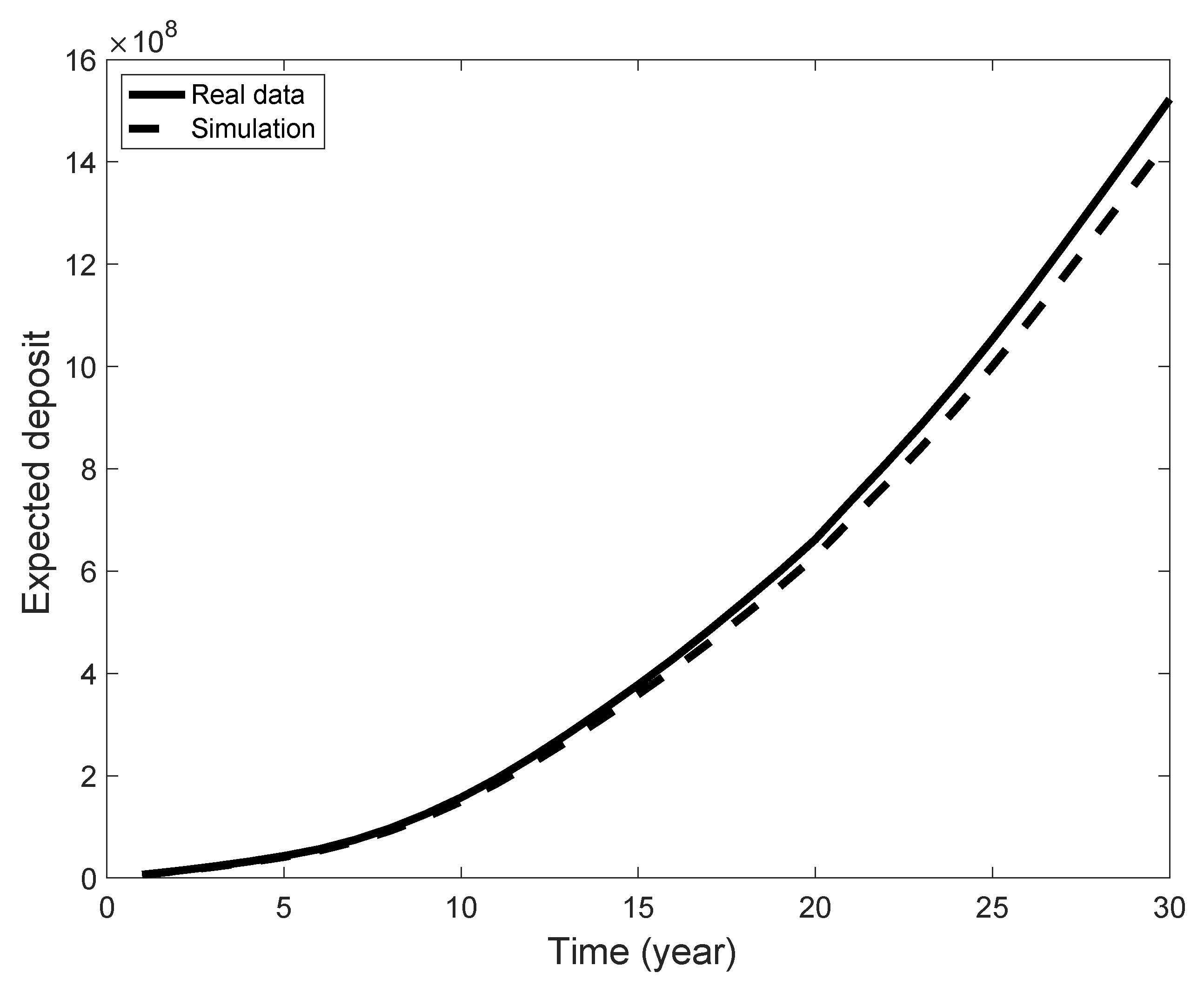More precisely, if the fund is composed at the initial time zero of K members allocated in the income classes according to the matrix $\mathbf{n}\left(0\right)={\left(n_{i,v}\left(0\right)\right)}_{i\in E,v\in \mathrm{I}{\mathrm{N}}^{*}}$ where $n_{i,v}\left(0\right)$ is the number of members that at Time 0 are in income level i with the duration of occupancy of this class equal to v, then the expected deposit is given by:

$$\sum _{v\ge 0}\sum _{i\in E}{n}_{i,v}\left(0\right)·V_i(v;t).$$

It should be mentioned that according to the general theory developed for semi-Markov systems, it is also possible to evaluate open systems, as done for example in McClean (1980); Papadopoulou et al. (2012); Papadopoulou and Vassiliou (1999).

4. Results and Discussion

In this section, we will try to implement a Markov process to describe the salary evolution of the active participants of the pension scheme. In particular, we are interested in finding out whether the model described in Section 3.1, i.e., a semi-Markov model with a backward reward process, is more suitable than a simple Markov chain to model salaries.

From the analysis of the graphs shown in the above paragraph, and in particular of the histogram of the average monthly salaries, we chose to divide salaries into 11 states. The first ten states were constructed considering salaries from 0–20,000 Euros and forming groups by a step of 2000 Euros, i.e., the first state considered the interval $[0,2000)$, the second one $[2000,4000)$, and so on. The last state was a residual class for salaries higher than 20,000 Euros.

The salary evolution can be modeled considering transitions from the above defined classes through a Markov process, which as mentioned before considers geometrically-distributed waiting times, or through a semi-Markov process, which permits the use of whatever type of distribution of the waiting times.

First, we estimated the transition probability matrices ${\tilde{p}}_{ij}$ of a Markov chain through its maximum likelihood estimator. To this end, we observed that in our applied problem, the income evolution of the K members was over a fixed observation period of length T. If we considered the observations from each member as independent and statistically identical copies, we can estimate the transition probability matrix as follows:

$${\tilde{p}}_{ij}=\frac{{\sum }_{n=1}^K{\sum }_{t=1}^T{\mathbf{1}}_{\{Z_{t-1}^{\left(n\right)}=i,Z_t^{\left(n\right)}=j\}}}{{\sum }_{j\in E}{\sum }_{n=1}^K{\sum }_{t=1}^T{\mathbf{1}}_{\{Z_{t-1}^{\left(n\right)}=i,Z_t^{\left(n\right)}=j\}}}=\frac{N_{ij}(T,K)}{N_i(T,K)}$$

(15)

where $N_{ij}(T,K),N_i(T,K)$ denote the number of times the process transitioned from a generic state i to another generic state j in the next time unit and the total number of times the process transitioned in the generic state i, respectively. As is possible to see from Equation (15), the transition probability matrix of the Markov chain was obtained by counting the number of transitions from every time to the successive one. The estimated matrix is:

$${\tilde{p}}_{ij}=\left(\begin{array}{ccccccccccc}0.676& 0.310& 0.012& 0.002& 0.001& 0.000& 0.000& 0.000& 0.000& 0.000& 0.000\\ 0.038& 0.797& 0.157& 0.006& 0.001& 0.000& 0.000& 0.000& 0.000& 0.000& 0.000\\ 0.003& 0.069& 0.789& 0.133& 0.005& 0.001& 0.000& 0.000& 0.000& 0.000& 0.000\\ 0.001& 0.008& 0.060& 0.806& 0.115& 0.007& 0.002& 0.000& 0.000& 0.000& 0.000\\ 0.000& 0.003& 0.008& 0.078& 0.774& 0.119& 0.011& 0.003& 0.001& 0.001& 0.001\\ 0.000& 0.004& 0.006& 0.012& 0.099& 0.724& 0.125& 0.020& 0.006& 0.002& 0.003\\ 0.000& 0.002& 0.004& 0.006& 0.018& 0.132& 0.649& 0.136& 0.031& 0.008& 0.013\\ 0.001& 0.006& 0.007& 0.005& 0.011& 0.037& 0.171& 0.534& 0.156& 0.039& 0.032\\ 0.000& 0.005& 0.007& 0.004& 0.015& 0.020& 0.061& 0.167& 0.450& 0.160& 0.113\\ 0.000& 0.007& 0.007& 0.005& 0.004& 0.023& 0.027& 0.051& 0.188& 0.395& 0.293\\ 0.001& 0.007& 0.006& 0.004& 0.011& 0.007& 0.018& 0.026& 0.036& 0.066& 0.817\end{array}\right)$$

The second step is that of modeling the salary evolution through a semi-Markovian process. In order to do so, first the transition probabilities $p_{ij}$ of the embedded Markov chain have to be estimated according to:

$${\widehat{p}}_{ij}=\frac{{\sum }_{n=1}^K{\sum }_{h=1}^{N^{\left(n\right)}\left(T\right)}{\mathbf{1}}_{\{J_{h-1}^{\left(n\right)}=i,J_h^{\left(n\right)}=j\}}}{{\sum }_{j\in E}{\sum }_{n=1}^K{\sum }_{h=1}^{N^{\left(n\right)}\left(T\right)}{\mathbf{1}}_{\{J_{h-1}^{\left(n\right)}=i,J_h^{\left(n\right)}=j\}}},$$

(16)

where $N^{\left(n\right)}\left(T\right)$ is the number of transitions in the $n^{\mathrm{th}}$ member of the pension scheme. Once the embedded Markov chain has been estimated, we need to estimate the distribution of the waiting times.

Let us firstly define the probability mass function of the sojourn times as follows:

$$\begin{array}{c}{g}_{ij}\left(t\right)=\mathbb{P}[T_{n+1}-T_n=t|J_n=i,J_{n+1}=j]=\hfill \\ \left\{\begin{array}{cc}{G}_{ij}\left(t\right)-G_{ij}(t-1)& \mathrm{if} t>1\hfill \\ G_{ij}\left(1\right)& \mathrm{if} t=1\hfill \end{array}\right.\hfill \end{array}$$

(17)

We considered a discrete time step of one year and calculated the waiting times for up to 20 years. Through an algorithm, we estimated the sojourn times on the data using the following:

$${\widehat{g}}_{ij}\left(t\right)=\frac{{\sum }_{n=1}^K{\sum }_{h=1}^{N_{ij}^{\left(n\right)}\left(T\right)}{\mathbf{1}}_{\{T_h^{\left(n\right)}-T_{h-1}^{\left(n\right)}=t,J_{h-1}^{\left(n\right)}=i,J_h^{\left(n\right)}=j\}}}{{\sum }_{n=1}^K{\sum }_{h=1}^{N_{ij}^{\left(n\right)}\left(T\right)}{\mathbf{1}}_{\{J_{h-1}^{\left(n\right)}=i,J_h^{\left(n\right)}=j\}}}$$

(18)

where $N_{ij}^{\left(n\right)}\left(T\right)$ denotes the number of transitions from state i to state j held by member n in the observational period $\{0,1,\dots ,T\}$.

In order to verify the semi-Markov hypothesis, a test proposed by Stenberg et al. (2006) can be applied. Obviously, the model can be considered Markovian if the sojourn times are geometrically distributed.

Under the geometric hypothesis, the equality $g_{ij}\left(1\right)(1-g_{ij}\left(1\right))-g_{ij}\left(2\right)=0$ must hold. Then, a sufficiently strong deviation from this equality has to be interpreted as evidence in favor of the semi-Markov model.

The test-statistic is the following:

$${\widehat{S}}_{ij}=\frac{\sqrt{N_{i,j}(T,N)}\left({\widehat{g}}_{ij}\left(1\right)(1-{\widehat{g}}_{ij}\left(1\right))-{\widehat{g}}_{ij}\left(2\right)\right)}{\sqrt{{\widehat{g}}_{ij}\left(1\right){(1-{\widehat{g}}_{ij}\left(1\right))}^2(2-{\widehat{g}}_{ij}\left(1\right))}}.$$

(19)

where ${\widehat{g}}_{ij}\left(x\right)$ is the empirical estimator of the probability $g_{ij}\left(x\right)$.

The results of the test statistic are shown in

Table 4. Test scores for the classes of salaries.

	j	1	2	3	4	5	6	7	8	9	10	11
i
1		n.a.	−3.59	3.88	0.58	0.57	0.43	n.a.	n.a.	n.a.	n.a.	n.a.
2		3.86	n.a.	−3.49	−0.15	2.09	1.41	−0.75	−0.19	1.83	n.a.	0,04
3		1.93	9.89	n.a.	2.73	1.84	1.50	1.28	−1.34	−0.15	0.82	n.a.
4		2.28	7.13	8.82	n.a.	3.94	−0.08	1.39	−0.56	0.69	0.47	−0.19
5		0.85	2.48	2.47	8.25	n.a.	3.94	2.10	0.53	−0.01	1.36	1.46
6		n.a.	1.06	1.47	1.70	5.78	n.a.	3.54	1.26	−0.81	1.25	0.14
7		n.a.	0.97	0.54	0.43	4.63	4.00	n.a.	1.89	1.19	0.79	3.08
8		n.a.	−0.40	−0.56	−0.65	−0.13	2.46	3.44	n.a.	3.81	−1.08	0.72
9		n.a.	−0.46	n.a.	−0.52	1.51	1.86	1.56	1.96	n.a.	−0.45	0.88
10		n.a.	n.a.	n.a.	n.a.	n.a.	−0.28	−0.79	3.05	1.42	n.a.	0.24
11		n.a.	2.86	2.39	1.73	1.26	1.21	1.84	0.11	0.36	1.97	n.a.

. It reports the score as calculated from Equation (19) for the eleven states of the salaries.

This statistic, under the geometric hypothesis $H_0$ (or Markovian hypothesis), has approximately the standard normal distribution. This means that large values of the test statistic suggest the rejection of the Markovian hypothesis in favor of the more general semi-Markov one. We applied this procedure to our data to execute tests at a significance level of $95\%$.

In

Table 5. Decision for the null hypothesis for classes of salaries. R, Rejected; A, Accepted.

	j	1	2	3	4	5	6	7	8	9	10	11
i
1		n.a.	R	R	A	A	A	n.a.	n.a.	n.a.	n.a.	n.a.
2		R	n.a.	R	A	R	A	A	A	A	n.a.	A
3		A	R	n.a.	R	A	A	A	A	A	A	n.a.
4		R	R	R	n.a.	R	A	A	A	A	A	A
5		A	R	R	R	n.a.	R	R	A	A	A	A
6		n.a.	A	A	A	R	n.a.	R	A	A	A	A
7		n.a.	A	A	A	R	R	n.a.	A	A	A	R
8		n.a.	A	A	A	A	R	R	n.a.	R	A	A
9		n.a.	A	n.a.	A	A	A	A	R	n.a.	A	A
10		n.a.	n.a.	n.a.	n.a.	n.a.	A	A	R	A	n.a.	A
11		n.a.	R	R	A	A	A	A	A	A	R	n.a.

, we show the results of the test applied to the waiting time distribution functions where R means the null hypothesis is $Rejected$, while A means that the null hypothesis of geometric distribution of the waiting times is $Accepted$.

As shown in Table 5, the geometric hypothesis was rejected for 31% of the waiting time distributions. There is, thus, evidence that we should be inclined to choose the more general model of a semi-Markov process over that of a simple Markov chain.

We also considered the case of the worker’s job qualification for the construction of the states of the salary process. The database furnished the necessary information regarding the different levels of qualification for each participant in each year of the observation period. In order to have an estimation as robust as possible, only qualifications with more then 5000 participants were considered.

The hypothesis under such modeling is that the transition from one qualification to the other, which would indirectly imply a transition in the salary level, can be described by a Markov process. The procedure applied was quite similar to the one described above. First, we estimated the transition probability matrix of the Markov chain through the same algorithm described above. The estimated matrix ${\widehat{p}}_{ij}$ is:

$$\left(\begin{array}{cccccccccccccccc}0.90& 0.03& 0.00& 0.01& 0.00& 0.02& 0.00& 0.00& 0.00& 0.00& 0.00& 0.00& 0.00& 0.00& 0.00& 0.03\\ 0.02& 0.92& 0.00& 0.01& 0.00& 0.01& 0.00& 0.00& 0.00& 0.00& 0.00& 0.00& 0.00& 0.00& 0.00& 0.03\\ 0.00& 0.11& 0.85& 0.01& 0.00& 0.01& 0.00& 0.00& 0.00& 0.00& 0.00& 0.00& 0.00& 0.00& 0.00& 0.01\\ 0.00& 0.03& 0.05& 0.89& 0.00& 0.01& 0.00& 0.00& 0.00& 0.00& 0.00& 0.00& 0.00& 0.00& 0.00& 0.01\\ 0.00& 0.01& 0.01& 0.11& 0.84& 0.01& 0.00& 0.00& 0.01& 0.00& 0.00& 0.00& 0.00& 0.00& 0.00& 0.01\\ 0.00& 0.01& 0.00& 0.03& 0.02& 0.91& 0.00& 0.00& 0.00& 0.00& 0.00& 0.00& 0.00& 0.00& 0.00& 0.01\\ 0.01& 0.01& 0.00& 0.03& 0.02& 0.47& 0.41& 0.01& 0.00& 0.02& 0.00& 0.00& 0.00& 0.00& 0.00& 0.01\\ 0.00& 0.01& 0.01& 0.01& 0.00& 0.09& 0.00& 0.78& 0.00& 0.02& 0.00& 0.00& 0.00& 0.00& 0.02& 0.05\\ 0.00& 0.02& 0.02& 0.02& 0.01& 0.01& 0.00& 0.00& 0.91& 0.00& 0.00& 0.00& 0.00& 0.00& 0.00& 0.01\\ 0.00& 0.01& 0.00& 0.02& 0.02& 0.38& 0.00& 0.01& 0.00& 0.52& 0.01& 0.00& 0.00& 0.00& 0.01& 0.02\\ 0.00& 0.00& 0.00& 0.00& 0.00& 0.01& 0.00& 0.00& 0.00& 0.00& 0.95& 0.00& 0.00& 0.00& 0.00& 0.03\\ 0.00& 0.00& 0.00& 0.00& 0.00& 0.00& 0.00& 0.00& 0.00& 0.00& 0.00& 0.97& 0.00& 0.00& 0.00& 0.02\\ 0.00& 0.01& 0.00& 0.01& 0.00& 0.07& 0.32& 0.02& 0.00& 0.03& 0.00& 0.00& 0.50& 0.00& 0.01& 0.02\\ 0.00& 0.01& 0.00& 0.01& 0.01& 0.05& 0.00& 0.01& 0.00& 0.61& 0.01& 0.00& 0.00& 0.24& 0.01& 0.04\\ 0.00& 0.01& 0.00& 0.00& 0.01& 0.03& 0.00& 0.01& 0.00& 0.14& 0.00& 0.00& 0.01& 0.63& 0.13& 0.04\\ 0.01& 0.01& 0.00& 0.01& 0.00& 0.04& 0.00& 0.01& 0.00& 0.02& 0.05& 0.00& 0.00& 0.01& 0.01& 0.81\end{array}\right)$$

Secondly, we supposed that a semi-Markov model could better explain the transitions between states since it gives the possibility of using whatever type of waiting time distribution.

The values of the statistic test were obtained in the same way as seen above and are reported in

Table 6. Test scores for the qualification states.

	j	1	2	3	4	5	6	7	8	9	10	11	12	13	14	15	16
i
1		n.a.	0.59	−0.50	−0.69	2.32	1.40	1.41	0.02	0.06	0.83	−0.43	n.a.	n.a.	n.a.	0.24	1.08
2		−0.10	n.a.	1.53	0.16	−0.08	1.96	0.82	−0.13	1.17	3.90	0.20	−0.30	n.a.	n.a.	1.22	2.72
3		1.67	−0.12	n.a.	0.95	0.68	1.38	n.a.	0.73	0.81	1.35	−0.25	n.a.	n.a.	0.82	0.27	0.90
4		−2.49	−0.95	−3.78	n.a.	0.85	3.27	0.19	−0.46	0.05	1.14	1.80	n.a.	n.a.	n.a.	0.00	1.41
5		1.24	1.79	0.97	−0.75	n.a.	2.87	1.97	1.48	−4.14	2.55	0.63	n.a.	n.a.	0.82	0.99	−0.24
6		2.30	0.93	−0.43	−2.36	−0.29	n.a.	5.11	1.58	−0.93	1.03	1.55	0.39	4.05	2.54	0.44	1.36
7		−1.44	−0.77	−0.57	−2.96	−1.94	−24.71	n.a.	0.09	−0.23	−1.99	−0.61	−2.27	0,00	n.a.	−0.52	−0,33
8		0.01	1.28	−0.02	1.87	0.88	0.83	3.19	n.a.	0.37	−0.73	−0.39	−0.55	n.a.	−0.15	−1.20	−0.56
9		0.14	1.04	−0.72	0.92	5.83	0.36	n.a.	0.56	n.a.	n.a.	−0.82	n.a.	n.a.	n.a.	−0.82	1.13
10		−1.52	−2.36	0.60	−3.81	−5.88	−48.41	2.19	0.31	−1.29	n.a.	−2.71	n.a.	n.a.	−1.62	−1.93	−3.28
11		−3.44	1.08	1.15	0.35	n.a.	−0.14	n.a.	−0.47	n.a.	0.23	n.a.	−0.19	n.a.	n.a.	−0.82	1.28
12		n.a.	n.a.	n.a.	−0.10	n.a.	−2.35	n.a.	n.a.	n.a.	n.a.	n.a.	n.a.	n.a.	n.a.	n.a.	0.72
13		−4.36	−7.13	−2.98	−8.26	−5.84	−19.77	−87.59	−8.11	−2.49	−8.39	−0.52	−1.41	n.a.	1.17	0.15	−8.14
14		0.23	0.78	−1.14	−0.33	0.75	−0.02	−0.68	−0.61	n.a.	−1.88	−1.22	−0.99	n.a.	n.a.	−0.07	0.43
15		−0.28	−0.16	n.a.	−1.94	−0.44	−0.60	−0.79	−0.19	−1.15	−9.53	−1.12	n.a.	n.a.	−2.18	n.a.	−1.12
16		−0.05	1.38	−0.78	0.56	1.87	4.18	0.10	2.33	−0.21	2.42	−31.66	0.62	−0.47	5.05	1.56	n.a.

. We fixed a level of significance of 95%, and the results of the statistic test are given in

Table 7. Decision for the null hypothesis for qualification states.

	j	1	2	3	4	5	6	7	8	9	10	11	12	13	14	15	16
i
1		n.a.	A	A	A	R	A	A	A	A	A	A	n.a.	n.a.	n.a.	A	A
2		A	n.a.	A	A	A	R	A	A	A	R	A	A	n.a.	n.a.	A	R
3		A	A	n.a.	A	A	A	n.a.	A	A	A	A	n.a.	n.a.	A	A	A
4		R	A	R	n.a.	A	R	A	A	A	A	A	n.a.	n.a.	n.a.	A	A
5		A	A	A	A	n.a.	R	R	A	R	R	A	n.a.	n.a.	A	A	A
6		R	A	A	R	A	n.a.	R	A	A	A	A	A	R	R	A	A
7		A	A	A	R	A	R	n.a.	A	A	R	A	R	A	n.a.	A	A
8		A	A	A	A	A	A	R	n.a.	A	A	A	A	n.a.	A	A	A
9		A	A	A	A	R	A	n.a.	A	n.a.	n.a.	A	n.a.	n.a.	n.a.	A	A
10		A	R	A	R	R	R	R	A	A	n.a.	R	n.a.	n.a.	A	A	R
11		R	A	A	A	n.a.	A	n.a.	A	n.a.	A	n.a.	A	n.a.	n.a.	A	A
12		n.a.	n.a.	n.a.	A	n.a.	R	n.a.	n.a.	n.a.	n.a.	n.a.	n.a.	n.a.	n.a.	n.a.	A
13		R	R	R	R	R	R	R	R	R	R	A	A	n.a.	A	A	R
14		A	A	A	A	A	A	A	A	n.a.	A	A	A	n.a.	n.a.	A	A
15		A	A	n.a.	A	A	A	A	A	A	R	A	n.a.	n.a.	R	n.a.	A
16		A	A	A	A	A	R	A	R	A	R	R	A	A	R	A	n.a.

. The null hypothesis of the geometric distribution was rejected for 25% of the waiting time distributions considered, and thus, we concluded that the semi-Markov process was more suitable to model the salary evolution of participants with states formed on the basis of the active workers’ qualification.

4.1. Markov versus Semi-Markov: An Alternative Test Based on Wilk’s Test

A more powerful test could be applied to test the Markov chain assumption against the semi-Markov alternative.1

To this end, we observed that if the model under the null hypothesis was a Markov chain with transition probabilities ${\tilde{p}}_{ij}$, then the following relation could be established with the corresponding semi-Markov kernel (see, e.g., Barbu and Limnios 2008):

$$q_{ij}\left(k\right)={\left({\tilde{p}}_{ii}\right)}^{k-1}·{\tilde{p}}_{ij},$$

from which it is simple to establish that:

$$p_{ij}=\frac{{\tilde{p}}_{ij}}{1-{\tilde{p}}_{ii}},$$

and consequently:

$$g_{ij}\left(k\right)=\frac{q_{ij}\left(k\right)}{p_{ij}}={\left({\tilde{p}}_{ii}\right)}^{k-1}·(1-{\tilde{p}}_{ii}).$$

(20)

Relation (20) shows that $g_{ij}\left(k\right)$, under the null hypothesis, is independent of j, and then, the equality:

$$g_{ij}\left(1\right)·(1-g_{ij}\left(1\right))=g_{ij}\left(2\right),$$

should be the same for all $j\in E$. The test proposed by Stenberg et al. (2006) ignored this fact and therefore can be improved by an alternative test that considers this additional property.

Informally, it would be possible to compare the log-likelihood function under the null hypothesis (Markov model) ${\mathcal{L}}_{MC}$ with that under the alternative hypothesis (semi-Markov model) ${\mathcal{L}}_{SMC}$. The specific form of this likelihood can be obtained for example in Sadek and Limnios (2002) and in Trevezas and Limnios (2011).

Once these values have been computed, a Wilk’s likelihood ratio test can be applied using the statistic:

$$D=2·({\mathcal{L}}_{SMC}-{\mathcal{L}}_{MC}),$$

which is approximately distributed as a chi-squared distribution with the degree of freedom equal to the difference between the number of free parameters of the semi-Markov model and those of the Markov chain model.

4.2. Results on Accumulated Rewards

According to Equation (14), it is possible to estimate, at Time 0, the total expected discounted amount of deposits due to the payments of all members of the fund up to time t. To do so, we fixed a constant discount factor $e^{-\delta }=1\%$ (a term structure of discount factors can also be simply used) and a the level of contribution, which is just a constant fraction of the salary, to $10\%$ for the whole time period t. Using the estimated probabilities, according to the previous section, we ran extensive Monte Carlo simulations and back tested the performance of the proposed model. In Figure 4, a comparison between real and simulated data is shown. We estimated the mean percentage absolute error between the two curves, obtaining a value of $5\%$, showing a good agreement between the data and model.

The analysis shows that the model can be useful to estimate the future reserve accumulated in the fund by giving a good prediction of the salary lines of the workers.

5. Conclusions

In this paper, we proposed a semi-Markov Chain with backward recurrence time to model salary lines. This is a more general model compared to the simple Markov chain since any type of distribution can be used for the waiting times, while the latter allows only the geometric distribution.

The model was applied to a dataset of active participants in the Italian Pension Scheme of the First Pillar. More than 27 thousand workers were observed over a period of 30 years. Salaries of participants were clustered to form the states of a stochastic process in two ways: the first one considered classes of salaries of 2000 Euros, while the second one was based on the qualification of the workers. In both cases, the transition probability matrices of the embedded Markov chain were estimated. Then, the semi-Markov hypothesis was tested by a statistical test applied in the recent literature. We fixed a significance level of 95% and performed the statistical test on the distribution of the waiting times. The null hypothesis of the geometric distribution was rejected for nearly 30% and 25% of the tests, in the two cases considered, and thus, we concluded that the semi-Markov model should be preferred to a simple Markov chain to model salary evolution of participants. The model was also used to estimate the total expected discounted amount of deposits and compared to real data, showing a good agreement.

Further extension could be the use of a non-homogeneous semi-Markov process, which can be used to take into account the variation of the mean salary due to digitalization, ICT, the employment of the big data technique, and other technological evolutions. This interesting generalization for future studies needs the development of specific procedure for testing the hypothesis of homogeneity against the more general non-homogeneity assumption. A departing point could be the application of a chi-squared-type test of homogeneity proposed by Vassiliou and Vasileiou (2013).

References

1. Barbu, Vlad, Michel Boussemart, and Nikolaos Limnios. 2004. Discrete time semi-Markov model for reliability and survival analysis. Communications in Statistics-Theory and Methods 33: 2833–68. [Google Scholar] [CrossRef]
2. Barbu, Vlad Stefan, and Nikolaos Limnios. 2008. Semi-Markov Chains and Hidden Semi-Markov Models toward Applications—Their Use in Reliability and DNA Analysis. Lecture Notes in Statistics. New York: Springer, vol. 191. [Google Scholar]
3. D’Amico, Guglielmo, Montserrat Guillen, and Raimondo Manca. 2009. Full backward non homogeneous semi-Markov processes for disability insurance models: A Catalunya real data application. Insurance: Mathematics and Economics 45: 173–9. [Google Scholar] [CrossRef]
4. D’Amico, Guglielmo, Jacques Janssen, and Raimondo Manca. 2010. Initial and final backward and forward discrete time non homogeneous semi-Markov processes credit risk models. Methodology and Computing in Applied Probability 12: 215–25. [Google Scholar] [CrossRef]
5. D’Amico, Guglielmo, Jacques Janssen, and Raimondo Manca. 2011. Duration Dependent Semi-Markov Models. Applied Mathematical Sciences 5: 2097–108. [Google Scholar]
6. D’Amico, Guglielmo. 2013. A semi-Markov approach to the stock valuation problem. Annals of Finance 9: 589–610. [Google Scholar] [CrossRef]
7. D’Amico, Guglielmo, Montserrat Guillen, and Raimondo Manca. 2013. Semi-Markov Disability Insurance Models. Communications in Statistics-Theory and Methods 42: 2172–88. [Google Scholar] [CrossRef]
8. D’Amico, Guglielmo, Filippo Petroni, and Flavio Prattico. 2015. Performance Analysis of Second Order Semi-Markov Chains: An Application to Wind Energy Production. Methodology and Computing in Applied Probability 17: 781–94. [Google Scholar] [CrossRef]
9. Janssen, Jacques, and Raimondo Manca. 1997. A realistic non-homogeneous stochastic pension funds model on scenario basis. Scandinavian Actuarial Journal 1997: 113–37. [Google Scholar] [CrossRef]
10. McClean, Sally I. 1980. A Semi-Markov model for a multigrade population with poisson recruitment. Journal of Applied Probability 17: 846–52. [Google Scholar] [CrossRef]
11. Papadopoulou, Aleka, and George Tsaklidis. 2007. Some Reward Paths in Semi-Markov Models with Stochastic Selection of the Transition Probabilities. Methodology and Computing in Applied Probability 9: 399–411. [Google Scholar] [CrossRef]
12. Papadopoulou, Aleka A., and Panagiotis C. G. Vassiliou. 1999. Continuous Time Non Homogeneous Semi-Markov Systems. In Semi-Markov Models and Applications. Edited by Jacques Janssen and Nikolaos Limnios. Boston: Springer. [Google Scholar]
13. Papadopoulou, Aleka A., George Tsaklidis, Sally McClean, and Lalit Garg. 2012. On the moments and the Distribution of the Cost of a semi-Markov Model for Healthcare Systems. Methodology and Computing in Applied Probability 14: 717–37. [Google Scholar] [CrossRef]
14. Sadek, Amr, and Nikolaos Limnios. 2002. Asymptotic properties for maximum likelihood estimators for reliability and failure rates of Markov chains. Communications in Statistics Theory and Methods 31: 1837–61. [Google Scholar] [CrossRef]
15. Slipsager, Søren Kærgaard. 2018. The real risk in pension forecasting. Scandinavian Actuarial Journal 2018: 250–73. [Google Scholar] [CrossRef]
16. Stenberg, Fredrik, Raimondo Manca, and Dmitrii Silvestrov. 2006. Semi-Markov reward models for disability insurance. Theory of Stochastic Processes 12: 239–54. [Google Scholar]
17. Stenberg, Fredrik, Raimondo Manca, and Dmitrii Silvestrov. 2007. An algorithmic approach to discrete time non-homogeneous backward semi-Markov reward processes with an application to disability insurance. Methodology and Computing in Applied Probability 9: 497–519. [Google Scholar] [CrossRef]
18. Trevezas, Samis, and Nikolaos Limnios. 2011. Exact MLE and asymptotic properties for nonparametric semi-Markov models. Journal of Nonparametric Statistics 23: 719–39. [Google Scholar] [CrossRef]
19. Vassiliou, Panagiotis, and Aglaia Vasileiou. 2013. Asymptotic behavior of the survival probabilities in an homogeneous semi-Markov model for the migration process in credit risk. Linear Algebra and its Applications 438: 2880–903. [Google Scholar] [CrossRef]
20. Wang, Suxin, Yi Lu, and Barbara Sanders. 2018. Optimal investment strategies and intergeneretional risk sharing for target benefit pension plans. Insurance: Mathematics and Economics 80: 1–14. [Google Scholar]
1.
The authors acknowledge an anonymous referee for suggesting this testing strategy.
Figure 1. Histogram of active workers by age.
Ijfs 07 00044 g001
Figure 2. Average monthly salaries of active participants.
Ijfs 07 00044 g002
Figure 3. Histogram of monthly salaries of active participants.
Ijfs 07 00044 g003
Figure 4. Expected deposit as a function of time.
Ijfs 07 00044 g004