Article

Forecasting Term Structure of Interest Rates in Japan

Graduate School of Economics, Nagoya University, Furo-cho, Chikusa-ku, Nagoya 464-8601, Japan
Int. J. Financial Stud. 2019, 7(3), 39; https://doi.org/10.3390/ijfs7030039
Submission received: 15 May 2019 / Revised: 26 June 2019 / Accepted: 1 July 2019 / Published: 8 July 2019

Abstract

:
In this paper, we examined and compared the forecast performances of the dynamic Nelson–Siegel (DNS), dynamic Nelson–Siegel–Svensson (DNSS), and arbitrage-free Nelson–Siegel (AFNS) models after the financial crisis period. The best model for the forecast performance is the DNSS model in the middle and long periods. The AFNS is inferior to the DNS model for long-period forecasting. In U.S. bond markets, AFNS is shown to be superior to DNS in the U.S. However, for Japanese data, there is no evidence that the AFNS is superior to the DNS model in the long forecast horizon.

1. Introduction

After the financial crisis, the Japanese economy faced an economic environment unlike it had ever experienced before. In January 2013, under the new governor of the central bank, the Bank of Japan began carrying out a new monetary policy framework. In general, this is called the “unconventional monetary policy”.
In this paper, we examine and compare forecast performances for Japanese Government Bonds (JGB) from the financial crisis onwards. To analyze the dynamics of JGB yield, we adopt the Dynamic Nelson–Siegel (DNS), Dynamic Nelson–Siegel–Svensson (DNSS), and Arbitrage-free Nelson–Siegel (AFNS) models. The former two models are curve-fitting models, which do not impose theoretical fundamentals such as arbitrage pricing theory. On the other hand, the last model imposes the arbitrage pricing theory and, thus, it is theoretically more rigorous than the former two models.
To forecast the future dynamics of the yield curves is a key concern of economists, policymakers, and those in the private sector, as the dynamics of the yields are considered to include the expectations of the market. If we can forecast the dynamics of the yield curve or term structure of interest rates, we may capture future fluctuations of the economic fundamentals. Therefore, forecasting the term structure of interest rates is a major step towards discerning the economic activity of a country.
This study provides one main result: The DNSS model is the best, among the three models, to forecast future yields; it outperforms the random walk model (a benchmark model) for 6- and 12-month forecasts. Moreover, the AFNS model is inferior to the DNS model for long forecast horizons, with evidence suggesting that the arbitrage-free assumption is not appropriate for long-period forecasting; although, Christensen et al. (2011) showed that the AFNS model is superior to the DNS in terms of forecasting performance.
The next sub-section reviews the literature. The organization of the paper is at end of the section.

Literature Review

The literature of the curve-fitting model started with the pioneering work of Nelson and Siegel (1987). Diebold and Li (2006) extended the cross-sectional Nelson–Siegel model to the time series. We refer to the Diebold–Li extension of Nelson–Siegel model as the dynamic Nelson-Siegel (DNS) model. The DNS model is a three-factor model. On the other hand, Diebold and Rudebusch (2013) introduced a four-factor1 model as an extension of the DNS. We refer to the four-factor model as the dynamic Nelson–Siegel–Svensson (DNSS) model.
A fundamental characteristic of curve-fitting models, such as DNS and DNSS, is that theoretically rigorous restrictions (like the arbitrage-free theory) are not imposed. Although this point has attracted criticism, Gasha et al. (2010) showed that these models have empirically better performances2 than arbitrage-free models; in particular, the affine term structure model, which was pioneered by Vasicek (1977). Cox et al. (1985) and Hull and White (1990) presented representative models that extend upon the Vasicek model. These arbitrage-free models impose the rigorous arbitrage-free theory. After Duffie and Kan (1996) derived the analytical solution of the affine term structure model, arbitrage-free models have rapidly developed (Ang and Piazzesi 2003). Since then, a lot of studies (Rudebusch and Wu 2008; Hördahl et al. 2005; Wu 2006; and Moench 2008) have been written on arbitrage-free macro-finance equilibrium models.
Fama (2006) discussed the forecasting of future spot rates by using the forward interest rate. Al-Zoubi (2009) examined a wide range of the interest rate models and reported the model parameter by using the generalized method of moment (GMM). De Rezende and Ferreira (2013) reported the improvement of the out-of-sample forecasts of the Nelson–Siegel class of models by using the quantile autoregression approach. There are a lot of the applied studies for the Nelson—Siegel class of models. Chen and Tsang (2013) applied the DNS model to domestic and foreign interest rate differential. Ishii (2018) extended the original Chen and Tsang (2013) model to the four- and five-factor models.
Christensen et al. (2009, 2011) set the Nelson–Siegel model into an affine term structure framework. Their model is called the arbitrage-free Nelson–Siegel (AFNS) model, which is considered to be both an empirically and theoretically good model. In fact, Christensen et al. (2011) and Diebold and Rudebusch (2013) showed that the AFNS was superior to the DNS for forecasting the performance of U.S. bond markets. Hence, they concluded that the imposition of the arbitrage-free theory improves the DNS.
There are many varieties of AFNS models. As Christensen et al. (2009, 2011) used, some are continuous time models3. Others (e.g., Alfaro 2011 and Niu et al. 2012) proposed discrete-time AFNS models. The advantage of the discrete model is that matching the data with the model is easier, such that we can estimate the model easily and simply.
A Kalman filter, through maximum likelihood estimation, is often used when estimating the parameters of the DNS and AFNS models. However, Hamilton and Wu (2012) pointed out that the maximum likelihood estimator might be a local estimator and, so, they suggested another method, such as the ordinary least squares (OLS) method. Diebold and Li (2006) and Niu et al. (2012) used the multiple regression method. Following these studies, our study employs the multiple regression method. In the first step, using the non-linear least-squares (NLS) method, the scale parameters of DNS, DNSS, and AFNS are estimated. In the second step, using OLS, the state variables are estimated.
Gurkaynak and Wright (2012) surveyed affine term structure models, including the Nelson–Siegel frameworks. Diebold and Rudebusch (2013) explained the framework of the DNS and the AFNS in detail.
Few studies have investigated JGB yields. One of the contributions of this study is to examine JGB yields and to compare the forecast performance of AFNS with those of DNS and DNSS. The second contribution is to provide evidence that the arbitrage-free assumption is not appropriate for the forecasting of JGB yields, unlike the forecasting of U.S. government bond yields.
The rest of this paper is organized as follows. In Section 2, we show the main theoretical models: DNS, DNSS, and AFNS. Section 3 characterizes the empirical models derived from the theoretical models. In Section 4, we show the data used in the analyses. Section 5 describes the empirical results. Our conclusions are drawn in Section 6.

2. Theoretical Model

This section explains three yield curve models: DNS, DNSS, and the discrete- and continuous-time versions of the AFNS model.

2.1. The Framework of the DNS and the DNSS Model

In the continuous-time model, the bond price P ( t , T ) of the maturity ( T t ) and the yield y ( t , T ) at time t are represented as:
P ( t , T ) = e ( T t ) y ( t , T ) .
The instantaneous forward rate is represented as:
f ( t , T ) = P ( t , T ) / ( T t ) P ( t , T ) .
Then, the yield is written as:
y ( t , T ) = 1 T t 0 T t f ( s , T ) d s .
Nelson and Siegel (1987) proposed the following forward rate:
f ( t , T ) = β 1 + β 2 e λ ( T t ) + β 3 ( T t ) λ e λ ( T t ) ,
where β and λ are parameters. This model is a three-factor model.
Substituting Equation (4) into Equation (3), we obtain the Nelson–Siegel yield function:
y ( t , T ) = β 1 + ( 1 e λ ( T t ) λ ( T t ) ) β 2 + ( 1 e λ ( T t ) λ ( T t ) e λ ( T t ) ) β 3 .
Svensson (1994) extended the three-factor Nelson-Siegel model to a four-factor model. In general, the extended version of the Nelson–Siegel model, which was proposed by Svensson (1994), is called the generalized Nelson–Siegel model. Its forward rate is written as:
f ( t , T ) = β 1 + β 2 e λ 1 ( T t ) + β 3 ( T t ) λ 1 e λ 1 ( T t ) + β 4 ( T t ) λ 2 e λ 2 ( T t ) .
Substituting Equation (6) into Equation (3), we obtain the Nelson–Siegel–Svensson yield:
y ( t , T ) = β 1 + ( 1 e λ 1 ( T t ) λ 1 ( T t ) ) β 2 + ( 1 e λ 1 ( T t ) λ 1 ( T t ) e λ 1 ( T t ) ) β 3 + ( 1 e λ 2 ( T t ) λ 2 ( T t ) e λ 2 ( T t ) ) β 4 .
Diebold and Li (2006) proposed the dynamic Nelson–Siegel model by allowing time-varying parameters. For convenience, we denote y ( t , T ) by y t ( τ ) with τ = T t . The DNS model is written as:
y t ( τ ) = β 1 t + β 2 t ( 1 e λ t τ λ t τ ) + β 3 t ( 1 e λ t τ λ t τ e λ t τ ) ,
where t denotes time.
Similarly, the DNSS is described as:
y t ( τ ) = β 1 t + β 2 t ( 1 e λ 1 t τ λ 1 t τ ) + β 3 t ( 1 e λ 1 t τ λ 1 t τ e λ 1 t τ ) + β 4 t ( 1 e λ 2 t τ λ 2 t τ e λ 2 t τ ) .
In the next section, we show the empirical models of Equations (8) and (9).

2.2. Affine Term Structure Model

In this sub-section, following Duffie and Kan (1996), we show the properties of the affine term structure model. Suppose that N state variables follow a vector autoregression(VAR)(1) process under the physical measure denoted by . The continuous representation of the VAR (1) process is:
d X t = κ ( θ X t ) d t + Σ d W t ,
where κ is an N × N matrix, θ is an N × 1 matrix, Σ is an N × N matrix, and W t is a Brownian motion under the physical measure . This form is called the Ornstein–Uhlenbeck process, as used in Vasicek (1977).
Suppose that the risk premium Γ t is defined in the essentially affine form, as proposed by Duffee (2002),
Γ t = Γ 0 + Γ 1 X t ,
where the scalar Γ 0 is a constant term, and Γ 1 is an N × 1 matrix.
Under the risk-neutral measure , the process d W t is defined4 as:
d W t = d W t + Γ t d t .
Substituting Equation (12) into Equation (10), the risk-neutral measure process of d X t is derived as:
d X t = κ ( θ X t ) d t + Σ d W ,
where κ is an N × N matrix, θ is an N × 1 matrix, and W is a Brownian motion under the risk-neutral measure .
Suppose that the instantaneous risk-free rate ( r ) is also an affine function:
r = ρ 0 + ρ 1 X t ,
where ρ 0 is a scalar and ρ 1 is a row vector.
The zero-coupon bond prices are an exponential affine function:
P ( t , T ) = exp [ B ( t , T ) X t + C ( t , T ) ] ,
where B ( t , T ) and C ( t , T ) are the solutions of the ordinary differential equations:
d B ( t , T ) d t = ρ 1 + ( κ ) B ( t , T ) ,   and
d C ( t , T ) d t = ρ 0 B ( t , T ) κ θ 1 2 j = 1 n ( Σ B ( t , T ) B ( t , T ) Σ ) ,
where n denote the number of the factor.
When B ( T , T ) = 0 and C ( T , T ) = 0 , the zero-coupon bond price P ( t , T ) is equal to one. This implies that the bond price corresponds with the par value at maturity, so that the boundary conditions are B ( T , T ) = 0 and C ( T , T ) = 0 . From the price function of the zero-coupon bond prices, the yield function is written as:
y ( t , T ) = log P ( t , T ) T t = B ( t , T ) T t X t C ( t , T ) T t .
This function is also the affine function. The details of the derivation are in Appendix A.

2.3. Continuous-Time AFNS Framework

In the previous two sub-sections, we have shown the derivations of DNS models and the affine term structure model. In this sub-section, following Christensen et al. (2011), we derived the AFNS model by combining the DNS model with the affine term structure model. In the three-factor model, the j -th elements of B ( t , T ) in Equation (18), denoted by B j , are as follows:
B 1 ( t , T ) = ( T t ) ,
B 2 ( t , T ) = 1 e λ ( T t ) λ ,
B 3 ( t , T ) = ( T t ) e λ ( T t ) 1 e λ ( T t ) λ .
Then, Equation (18) is written as
y ( t , T ) = X t 1 + [ 1 e λ ( T t ) λ ( T t ) ] X t 2 + [ 1 e λ ( T t ) λ ( T t ) e λ ( T t ) ] X t 3 C ( t , T ) T t .
This equation matches DNS model, except for the last term—which is often called the yield adjustment term or Jensen’s inequality term. This term arises from the convexity of the function and plays a role describing the non-linearity of the yield curve.
When we suppose the three-factor model, Equations (16) and (17) are rewritten as:
d B ( t , T ) d t = ρ 1 + ( κ ) B ( t , T ) ,
d C ( t , T ) d t = ρ 0 B ( t , T ) κ θ 1 2 j = 1 3 ( Σ B ( t , T ) B ( t , T ) Σ ) .
From Equation (23) and the relationship
d d t [ e ( κ ) ( T t ) B ( t , T ) ] = e ( κ ) ( T t ) d B ( t , T ) d t e ( κ ) ( T t ) ( κ ) B ( t , T ) ,
we obtain
d d t [ e ( κ ) ( T t ) B ( t , T ) ] = e ( κ ) ( T t ) ρ 1 .
Integrating Equation (26), we get:
t T d d s [ e ( κ ) ( T s ) B ( s , T ) ] d s = t T e ( κ ) ( T s ) ρ 1 d s .
From the boundary condition B ( T , T ) = 0, the solution is:
B ( t , T ) = e ( κ ) ( T s ) t T e ( κ ) ( T s ) ρ 1 d s .
When we impose the following structure5,
κ = [ 0 0 0 0 λ 0 0 λ λ ] ,
and
ρ 0 = 0 ,   ρ 1 = [ 1 1 0 ] .
From the structures (30) and (31),
e ( κ ) ( T t ) = [ 1 0 0 0 e λ ( T t ) 0 0 λ ( T t ) e λ ( T t ) e λ ( T t ) ] .
Substituting above results into the ordinary differential equation system (29), we obtain:
B ( t , T ) = [ 1 0 0 0 e λ ( T t ) 0 0 λ ( T t ) e λ ( T t ) e λ ( T t ) ] × t T [ 1 e λ ( T t ) λ ( T t ) e λ ( T t ) ] d s ,
and the solution is:
B ( t , T ) = [ ( T t ) 1 e λ ( T t ) λ ( T t ) e λ ( T t ) 1 e λ ( T t ) λ ] .
Each element of Equation (33) corresponds to Equations (19)–(21), respectively, such that we can set the DNS model into the affine term structure model, except for the term C ( t , T ) .
Next, we consider the yield adjustment term C ( t , T ) / ( T t ) . From Equation (24), we can analytically derive the yield adjustment term. In the risk-neutral measure , θ is zero. Therefore, the yield adjustment term is:
C ( t , T ) T t = 1 2 ( T t ) j = 1 3 t T ( Σ B ( t , T ) B ( t , T ) Σ ) d s .
As for the dynamics of the state transition equations, there are two patterns in the yield adjustment term, depending on whether the factor dynamics are independent or correlated. If the state factor has independent factor dynamics, the volatility matrix Σ is represented as:
Σ = [ σ 11 0 0 0 σ 22 0 0 0 σ 33 ] .
Then, the yield adjustment term is written as:
C ( t , T ) T t = A ¯ ( ( T t ) 2 6 ) + B ¯ ( 1 2 λ 2 1 λ 3 1 e λ T t T t + 1 4 λ 3 1 e 2 λ T t T t ) + C ¯ ( 1 2 λ 2 + 1 λ 2 e λ ( T t ) 1 4 λ ( T t ) e 2 λ ( T t ) 3 4 λ 2 e 2 λ ( T t ) 2 λ 3 1 e λ ( T t ) T t 2 8 λ 3 1 e 2 λ ( T t ) T t ) ,
where:
A ¯ = σ 11 2 + σ 12 2 + σ 13 2 ,
B ¯ = σ 21 2 + σ 22 2 + σ 23 2 ,
C ¯ = σ 31 2 + σ 32 2 + σ 33 2 .
On the other hand, if the factor dynamics are correlated, the volatility matrix Σ is represented as6:
Σ = [ σ 11 σ 12 σ 13 σ 21 σ 22 σ 23 σ 31 σ 32 σ 33 ] .
Then, the yield adjustment term is:
C ( t , T ) T t = A ¯ ( ( T t ) 2 6 ) + B ¯ ( 1 2 λ 2 1 λ 3 1 e λ ( T t ) T t + 1 4 λ 3 1 e 2 λ ( T t ) T t ) + C ¯ ( 1 2 λ 2 + 1 λ 2 e λ ( T t ) 1 4 λ ( T t ) e 2 λ ( T t ) 3 4 λ 2 e 2 λ ( T t ) 2 λ 3 1 e λ ( T t ) T t + 5 8 λ 3 1 e 2 λ ( T t ) T t ) + D ¯ ( 1 2 λ ( T t ) + 1 λ 2 e λ ( T t ) 1 λ 3 1 e λ ( T t ) T t ) + E ¯ ( 3 λ 2 e λ ( T t ) + 1 2 λ ( T t ) + 1 λ ( T t ) e λ ( T t ) 3 λ 3 1 e λ ( T t ) T t + F ¯ ( 1 λ 2 + 1 λ 2 e λ ( T t ) 1 2 λ 2 e 2 λ ( T t ) 3 λ 3 1 e λ ( T t ) T t + 3 4 λ 3 1 e λ ( T t ) T t ) ,
where:
D ¯ = σ 11 σ 21 + σ 12 σ 22 + σ 13 σ 23 ,
E ¯ = σ 11 σ 31 + σ 12 σ 32 + σ 13 σ 33 ,
F ¯ = σ 21 σ 31 + σ 22 σ 32 + σ 23 σ 33 .
The details of the derivation of Equations (36) and (38) are in Appendix A.
The yield adjustment term depends only on the time of maturity τ   ( = T t ) . Therefore, it is a constant value with time t . Moreover, as the maturity becomes larger, the value of the yield adjustment term is larger.

2.4. Discrete-Time AFNS

As it is easier to match data with a discrete AFNS model, rather than with the continuous version, we derive the discrete-time AFNS model, following Niu et al. (2012). Under the physical measure , the dynamics of the state variables are written as:
X t = μ + A X t 1 + η t ,
where η t   ~   N ( 0 , Q ) . Under the risk-neutral measure , the dynamics of the state variables are written as:
X t = μ + A X t 1 + η t ,
where η t   ~   N ( 0 , Q ) . The discrete versions7 of Equations (23) and (24) are represented as:
B ( t , T ) = ρ 1 k = 0 T t 1 ( Φ ) k   and
C ( t , T ) = C ( t , T 1 ) + C ( t , T 1 ) θ + 1 2 C ( t , T 1 ) Q C ( t , T 1 ) ,
where:
ρ 1 = [ 1 1 e λ λ 1 e λ λ e λ ] ,
and:
( Φ ) k = [ 1 0 0 0 e λ λ e λ 0 0 e λ ] k = [ 1 0 0 0 e k λ k λ e k λ 0 0 e k λ ] .
From Equations (41) and (44), we obtain:
B ( t , T ) = ρ 1 k = 0 T t 1 ( Φ ) k = [ n 1 e λ n λ n e λ n 1 e λ n λ ] .
We have that Equation (45) is the discrete version of Equation (33).
Moreover, in the risk-neutral measure , θ = 0 . Therefore, the yield adjustment term of the discrete version is written as:
C ( t , T ) = C ( t , T 1 ) + 1 2 C ( t , T 1 ) Q C ( t , T 1 ) .
Substituting Equations (43) and (44) into Equation (19), we obtain the discrete-time AFNS model as:
y ( t , T ) = X t 1 + [ 1 e λ ( T t ) λ ( T t ) ] X t 2 + [ 1 e λ ( T t ) λ ( T t ) e λ ( T t ) ] X t 3 C ( t , T ) T t ,
where C ( t , T ) is given by Equation (46).
Until now, we have shown theoretical models of DNS, DNSS, and AFNS (continuous- and discrete-time versions). In the next section, we show empirical models of Equations (8), (9), and (45). Moreover, we compare the forecast performances of the yields.

3. Empirical Models

For the purpose of evaluating forecasting performance of the three yield curve models, it is convenient to represent the empirical counterparts of the theoretical models explicitly.
As we cannot observe the state variables, we must estimate them first. As Piazzesi (2010) used, the most frequently used way of estimating state variables is to use the principal component method. As Litterman and Scheinkman (1991) first showed, it is usually considered that the yield curve is explained almost by the first principal components. Moreover, the first, second, and third components are usually identified as the level, slope, and curvature of the yield curve, respectively.
In this paper, we supposed that the transition equation of the state variables followed a VAR (1) process, and that the state variables were uncorrelated or correlated with each other. The uncorrelated transition equation of the state variables is represented as:
[ X t 1 , D N S X t 2 , D N S X t 3 , D N S ] = ( I A ) μ + [ A 11 0 0 0 A 22 0 0 0 A 33 ] [ X t 1 1 , D N S X t 1 2 , D N S X t 1 3 , D N S ] + [ η t 1 η t 2 η t 3 ] ,
where μ is a vector of means. The variance–covariance matrix of the stochastic shocks is represented as:
Q D N S = [ Q 11 0 0 0 Q 22 0 0 0 Q 33 ] .
From Equation (8), the empirical model of DNS is represented as:
[ y t ( τ 1 ) y t ( τ 2 ) y t ( τ N ) ] = [ 1 1 e λ τ 1 λ τ 1 1 e λ τ 1 λ τ 1 e λ τ 1 1 1 e λ τ 2 λ τ 2 1 e λ τ 2 λ τ 2 e λ τ 2 1 1 e λ τ N λ τ N 1 e λ τ N λ τ N e λ τ N ] [ X t 1 , D N S X t 2 , D N S X t 3 , D N S ] + [ ε t ( τ 1 ) ε t ( τ 2 ) ε t ( τ N ) ] ,
where ε t ( τ i ) is the measurement error and i.i.d. white noise and τ N denotes a maturity N .
Similarly, we consider the uncorrelated state dynamics for the DNSS,
[ X t 1 , D N S S X t 2 , D N S S X t 3 , D N S S X t 4 , D N S S ] = ( I A ) µ + [ A 11 0 0 0 0 A 22 0 0 0 0 A 33 0 0 0 0 A 44 ] [ X t 1 1 , D N S S X t 1 2 , D N S S X t 1 3 , D N S S X t 1 4 , D N S S ] + [ η t 1 η t 2 η t 3 η t 4 ] ,
where the variance–covariance matrix of the stochastic shocks is represented as:
Q D N S S = [ Q 11 0 0 0 0 Q 22 0 0 0 0 Q 33 0 0 0 0 Q 44 ] .
From Equation (9), the empirical model of DNSS is represented as:
[ y t ( τ 1 ) y t ( τ 2 ) y t ( τ N ) ] = [ 1 1 e λ 1 τ 1 λ 1 τ 1 1 e λ 1 τ 1 λ τ 1 e λ 1 τ 1 1 e λ 2 τ 1 λ 2 τ 1 e λ 2 τ 1 1 1 e λ 1 τ 2 λ 1 τ 2 1 e λ 1 τ 2 λ 1 τ 2 e λ 1 τ 2 1 e λ 2 τ 2 λ 2 τ 2 e λ 2 τ 2 1 1 e λ 1 τ N λ 1 τ N 1 e λ 1 τ N λ 1 τ N e λ 1 τ N 1 e λ 2 τ N λ 2 τ N e λ 2 τ N ] [ X 1 , D N S S X 2 , D N S S X 3 , D N S S X 4 , D N S S ] + [ ε t ( τ 1 ) ε t ( τ 2 ) ε t ( τ N ) ] .
From Equation (39), suppose that the state transition equation of AFNS also follows a VAR (1) process, as in DNS:
[ X t 1 , A F N S X t 2 , A F N S X t 3 , A F N S ] = ( I A ) μ + [ A 11 0 0 0 A 22 0 0 0 A 33 ] [ X t 1 1 , A F N S X t 1 2 , A F N S X t 1 3 , A F N S ] + [ η t 1 η t 2 η t 3 ] ,
where the stochastic shock variance–covariance matrix is represented as:
Q A F N S = [ Q 11 0 0 0 Q 22 0 0 0 Q 33 ] .
From Equation (45), the empirical model of AFNS is represented as:
[ y t ( τ 1 ) y t ( τ 2 ) y t ( τ N ) ] = [ 1 1 e λ τ 1 λ τ 1 1 e λ τ 1 λ τ 1 e λ τ 1 1 1 e λ τ 2 λ τ 2 1 e λ τ 2 λ τ 2 e λ τ 2 1 1 e λ τ N λ τ N 1 e λ τ N λ τ N e λ τ N ] [ X t 1 , A F N S X t 2 , A F N S X t 3 , A F N S ] C ( t , T ) T t + [ ε t ( τ 1 ) ε t ( τ 2 ) ε t ( τ N ) ] .
There is a yield adjustment term C ( t , T ) / ( T t ) in this equation, which generates a different forecast than the DNS model. Simply stated, the arbitrage-free condition imposes this term, which is a feature of the AFNS and affine term structure models that distinguishes them from curve-fitting models. The derivation of the AFNS model, in detail, is in Appendix A.
Next, we considered the correlated transition equation of the state variables. The representations of the state transition equation of the correlated state variables are as follows:
A D N S = [ A 11 A 12 A 13 A 21 A 22 A 23 A 31 A 32 A 33 ] ,
A D N S S = [ A 11 A 12 A 13 A 14 A 21 A 22 A 23 A 23 A 31 A 32 A 33 A 34 A 41 A 42 A 43 A 44 ] ,
A A F N S = [ A 11 A 12 A 13 A 21 A 22 A 23 A 31 A 32 A 33 ] .
The variance-covariance matrixes of η t are written as:
Q D N S = [ Q 11 Q 12 Q 13 Q 21 Q 22 Q 23 Q 31 Q 32 Q 33 ] ,
Q D N S S = [ Q 11 Q 12 Q 13 Q 14 Q 21 Q 22 Q 23 Q 23 Q 31 Q 32 Q 33 Q 34 Q 41 Q 42 Q 43 Q 44 ] ,
Q A F N S = [ Q 11 Q 12 Q 13 Q 21 Q 22 Q 23 Q 31 Q 32 Q 33 ] .
Even though each state variable is correlated, the empirical DNS, DNSS, and AFNS models have the same representation.
In summary, we can write the above equation simply, in matrix representation. Each state transition equation of the DNS, DNSS, and AFNS models, in matrix form, is represented as:
X t = ( I A ) μ + A X t 1 + H t ,
where X t is a 3 × 1 matrix (DNS and AFNS) or 4 × 1 matrix (DNSS), A is a state transition matrix of 3 × 3 (DNS and AFNS) or 4 × 4 (DNSS), H t is a N × 1 matrix such that H t   ~   N ( 0 , Q ) , and Q is a variance–covariance matrix of 3 × 3 (DNS and AFNS) or 4 × 4 (DNSS).
In matrix representation, the empirical DNS and DNSS models are represented as:
Y t = B X t + Ε t ,
where Y t is a N × 1 matrix, B t is a matrix of 3 × N (DNS) or 4 × N (DNSS), and Ε t is a N × 1 matrix such that Ε t   ~   N ( 0 , I ) .
On the other hand, the empirical model of AFNS is represented as:
Y t = B X t + C + Ε t ,
where C is the yield adjustment term, which is a N × 1 matrix corresponding to the term C ( t , T ) / ( T t ) in Equation (23) or (45).

4. Estimation

In this section, we explained the details of the data used in the empirical analysis and report the estimated parameters and the state variables of the DNS, DNSS, and AFNS models. We employed monthly JGB zero-coupon yield from September 2009 to June 2015. The zero-yields were calculated8 using the treasury discount bill and the prevailing interest rates, published by the Ministry of Finance. The maturities are 3, 6, 12, 24, 36, 48, 60, 72, 84, 96, 108, 120, 180, 240, 300, 360, and 480 months. Figure 1 is the JGB zero-yield curve (September 2009 to June 2015).
In the first step, we estimated the scale parameters λ , λ 1 , and λ 2 for the DNS and DNSS models using non-linear least-squares. In the second step, we estimated the state variables for the DNS and DNSS models using the estimated parameters λ , λ 1 , and λ 2 , and OLS. Moreover, we estimated the transition matrix A and the variance–covariance matrix Q for each independent and correlated state variable. The estimated state variables for DNS are invalid for using for the AFNS, since the constant term includes a bias. Using the estimated variance–covariance matrix, we could obtain the values of C ( t , T ) / ( T t ) from Equation (42). Subtracting the yield adjustment term C ( t , T ) / ( T t ) from the yields, we excluded the constant term bias, so that we could estimate the state variable for the AFNS model.

4.1. Estimation of the Values of λ

In this sub-section, we estimated the scale parameters λ , λ 1 , and λ 2 of the DNS and DNSS models (Equations (5) and (7)). The estimation method was non-linear least-squares. As this model is a numerical approximation method, we needed to determine the initial values of the parameters. We set the initial values as X 1 = X 2 = X 3 = X 4 = 0 , λ = λ 1 = 0.0327 9, and λ 2 = 0.01635 10. The Levenberg–Marquardt algorithm was used to approximate the values numerically.
As the DNS and DNSS are time-series models, we approximated each parameter, using non-linear least-squares, at each time point. The estimated DNS and DNSS models are written as:
y ^ t ( τ ) = β ^ 1 , t + β ^ 2 , t ( 1 e λ ^ t τ λ ^ t τ ) + β ^ 3 , t ( 1 e λ ^ t τ λ ^ t τ e λ ^ t τ ) ,
and:
y ^ t ( τ ) = β ^ 1 , t + β ^ 2 , t ( 1 e λ ^ 1 , t τ λ ^ 1 , t τ ) + β ^ 3 , t ( 1 e λ ^ 1 , t τ λ ^ 1 , t τ e λ ^ 1 , t τ ) + β ^ 4 , t ( 1 e λ ^ 2 , t τ λ ^ 2 , t τ e λ ^ 2 , t τ ) ,
respectively.
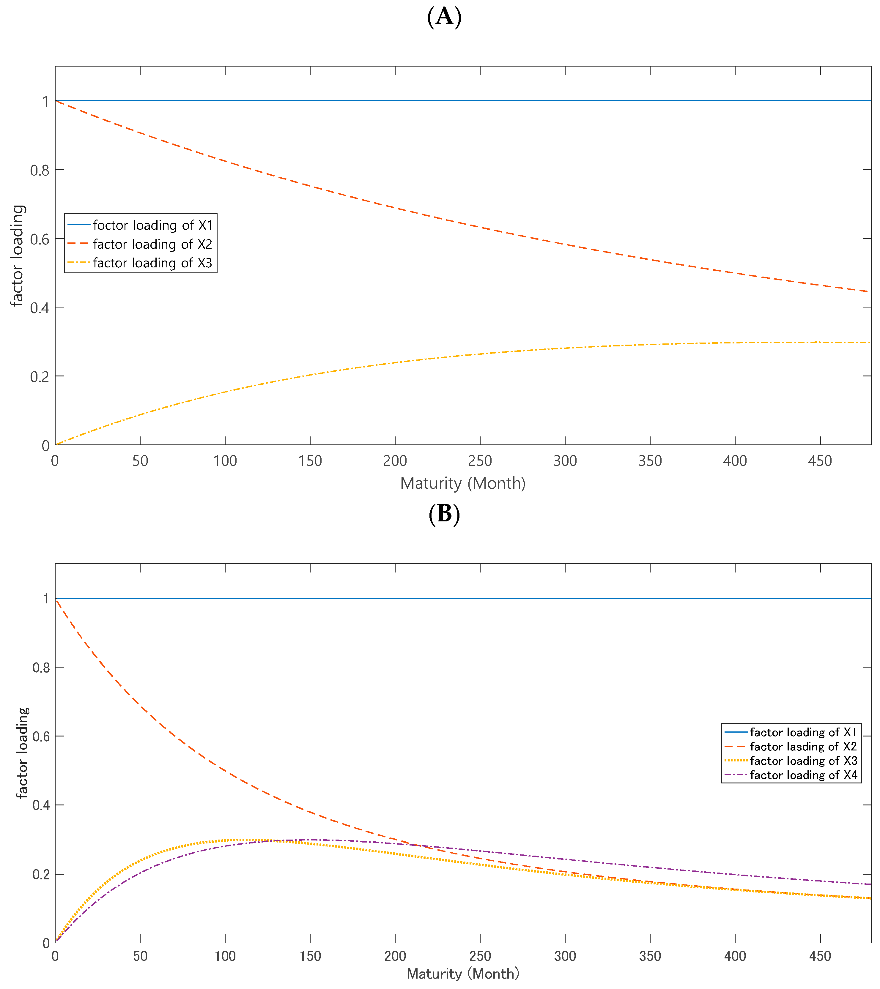
In the DNS and DNSS models, the parameters λ ^ , λ ^ 1 , and λ ^ 2 changed over time. However, in previous studies (Diebold and Li (2006); Christensen et al. (2011), and Diebold and Rudebusch (2013)), the parameters were defined to be constant throughout time, as the fluctuation of the values is small in each time point and to ensure the stability of the estimation results. Therefore, we adopted the averages of λ ^ t , λ ^ 1 , t , and λ ^ 2 , t as the parameters λ , λ 1 , and λ 2 , respectively. From the estimation, we obtained the estimated parameters11 λ = 0.004 , λ 1 = 0.016 , and λ 2 = 0.012 . Moreover, suppose that the value λ of the DNS model was identical to λ in the AFNS model12. From the estimated λ , λ 1 , and λ 2 , the factor loadings on β 1 , β 2 , β 3 , and β 4 of the DNS and DNSS models were calculated. Then, X 1 , X 2 , X 3 , and X 4 was simply a rewriting of each β .
The dynamics of the factor loadings through the maturity τ are described in Figure 2. Figure 2A shows the dynamics of the factor loadings of the DNS model and Figure 2B shows the dynamics of those of the DNSS model. The first factor loading is a constant through the maturity. The second factor loading starts at 1 and goes to 0 gradually, so that it affects short-term yields. The third factor loading starts at 0 and rises in the medium-term, after which it goes to 0 again. The fourth factor loading also starts 0. Its dynamics are initially the same as the third factor. However, the fourth factor loading affects longer-term yields than the third factor loading. As we can see from the above results, the second factor loading was a short-term factor, the third was a medium-term factor, and the fourth was a medium- to long-term factor.

4.2. Estimation of Latent State Variables

In the previous sub-section, we specified the values of λ , λ 1 , and λ 2 . In this sub-section, we estimated the unobservable state variables of the DNS, DNSS, and AFNS models. However, the AFNS model includes a constant term. Hence, we cannot use the state variables of the DNS model13 for the AFNS model, due to the constant term bias. The estimation method for the AFNS model was described later. Here, we carried on the estimation of the second step. If we estimated the parameters without separating between the first step and the second step (i.e., using one-step estimation), we needed to use a state space estimation, such as a Kalman filter. This method imposes a large burden numerically and it is possible that the estimation result is only locally convergent. On the other hand, if we used the multiple regression method, once the value of λ was determined, we could estimate the state variables easily using OLS and, so, we separated the estimation: The first step14 estimated the scale parameter λ , and the second step estimated the state variables using the value obtained in the first step.
First, we considered the estimation of the state variables in the DNS and DNSS models. Taking the values of λ , λ 1 , and λ 2 as above and substituting them into Equations (66) and (67), the parameters β ^ 1 , t , β ^ 2 , t , β ^ 3 , t , and β ^ 4 , t were estimated using ordinary least-squares at any one point. Moreover, since the estimated β ^ i , t corresponds to the unobservable variables at each time-point, the time-series of each estimated parameter was regarded as the time series of the state variables. Therefore, we redefined the parameters, ( β ^ 1 , t D N S , β ^ 2 , t D N S , β ^ 3 , t D N S ) and ( β ^ 1 , t D N S S , β ^ 2 , t D N S S , β ^ 3 , t D N S S , β ^ 4 , t D N S S ) as ( X ^ 1 , t D N S , X ^ 2 , t D N S , X ^ 3 , t D N S ) and ( X ^ 1 , t D N S S , X ^ 2 , t D N S S , X ^ 3 , t D N S S , X ^ 4 , t D N S S ).
Next, we explained how we estimated the state variables in AFNS. Although the number of the state variables was the same as the DNS model, the AFNS includes the constant term C , as shown in Equation (63). Therefore, we could not directly apply the estimated state variables in the DNS to the AFNS, as such a method causes the constant term bias. To correct the bias, we needed to estimate the state variables after subtracting the constant term from the yield.
Defining Z ^ t ( τ ) y ^ t ( τ ) C ^ , we have:
Z ^ t ( τ ) = X ^ 1 , t + X ^ 2 , t ( 1 e λ τ λ τ ) + X ^ 3 , t ( 1 e λ t τ λ τ e λ τ ) ,
from Equation (47).
We obtained the estimate C ^ from Equation (46), assuming that the variance–covariance matrix Q of the AFNS model was the same as that of the DNS model. As we assumed that the parameter λ of the AFNS model should be the same as that of the DNS model, we could apply the OLS method to Equation (68).
Table 1 reports the mean, standard deviation, and the 1- and 12-month lag autocorrelations of the estimated state variables for the DNS, DNSS, and AFNS models. In the state variables for the DNS and DNSS models, there was no difference between the independent or correlated cases, since the state variables were identical.
We saw two remarkable features in the AFNS model. First, regardless of whether the yield adjustment term was independent or correlated, the state variable had a strong auto-correlation with the 1-month lag. Second, the auto-correlation decayed with the 12-month lag. The sign of the mean was the same between the first and second state variables of the DNS and AFNS models.

4.3. Estimation of the Transition Matrix

Now, we proceeded to the estimation of the transition matrix A in Equations (48), (51), and (54). In this estimation, the data set was the estimated state variables of the previous sub-section. When estimating Equation (48), the covariance matrix Q was estimated as the sample covariance matrix of the error terms. Table 2 reports the estimation results for the transition matrix and Table 3 reports the variance–covariance matrix.
As Table 2 indicates, almost all of the diagonal elements of the transition matrix were statistically significant in all models. Note that, by assumption, the transition matrix of each DNS model was identical to that of the AFNS model, and that the covariance matrix Q of the AFNS model was identical to that of the DNS model.
As already explained in Section 4.2, we could calculate the yield adjustment term C of the AFNS model from the estimated variance–covariance matrix Q . However, due to large volatility, the yield adjustment term of the AFNS model with independent error term became too huge. Each element of the variance–covariance matrix was from two to ten times larger than what Christensen et al. (2011)15 obtained using U.S. data. For example, our estimated Q results in a yield adjustment term of about 20,000 bps for a 480-month maturity. As this is extremely unrealistic, in what follows, we omitted the results of the AFNS model with independent error terms.

5. Results: Forecasting Performances of the Three Models

In this section, we estimated the root mean square forecast error (RMSFE) of the 1-month, 3-month, 6-month, and 12-month forecasts for each of the three models.

5.1. Out-of-Sample Forecasting: Comparison of Forecasting Performances

We defined the h period forecast of the yield with maturity tau at time t as y t + h , t ( τ ) . As in Christensen et al. (2011), the forecasting measurement equations of the three models are written, respectively, as:
y t + h , t D N S ( τ ) = E [ y t + h ( τ ) ] = E [ X 1 ^ t + h ] + E [ X 2 ^ t + h ] ( 1 e λ τ λ τ ) + E [ X 3 ^ t + h ] ( 1 e λ τ λ τ e λ τ ) .
y t + h , t D N S S ( τ ) = E [ X 1 ^ t + h ] + + E [ X 2 ^ t + h ] ( 1 e λ 1 τ λ 1 τ ) + E [ X 3 ^ t + h ] ( 1 e λ 1 τ λ 1 τ e λ 1 τ ) + E [ X 4 ^ t + h ] ( 1 e λ 1 τ λ 1 τ e λ 1 τ ) ,
y t + h , t A F N S ( τ ) = E [ y t + h ( τ ) ] = E [ X 1 ^ t + h ] + E [ X 2 ^ t + h ] ( 1 e λ τ λ τ ) + E [ X 3 ^ t + h ] ( 1 e λ τ λ τ e λ τ ) C ^ ( τ ) τ ,
where C ^ ( τ ) τ is the yield adjustment term. As the transition dynamics are first-order, we can write the expectation of the state variables at t + h as:
E [ X t + h ] = ( i = 0 h 1 A i ) ( I A ) μ + A h X t ,
where X t denotes the column vector of the state variables. In this paper, we employed the random walk model (without a drift term) as a benchmark model. This paper investigated the 1-, 3-, 6-, and 12-month ahead forecast ( h = 1,3,6,12). In out-of-sample forecast, these models were estimated only one time over the full sample periods (September 2009 to June 201516) and then used for forecasting h -month ahead horizon ( h = 1,3,6,12).
Table 4, Table 5, Table 6 and Table 7 report the root mean square forecast error (RMSFE)17 of the 1-, 3-, 6-, and 12-month forecasts, respectively. In the tables, the smallest RMSFE is boxed for each maturity and horizon. As these tables show, DNSS was clearly the best forecasting model among the three models for 6- and 12-month forecast horizons. Between two types of the DNSS models, the DNSS model based on the transition equation of the independent (uncorrelated) state variable was superior to the correlated model. It is clear to see that all of the off-diagonal elements of the transition matrix were statistically highly significant in the DNSS model. This superiority is plausible, because the DNSS model is theoretically the generalized model of the DNS model. We can say that the generality of the DNSS model was confirmed by our result. On the other hand, the random walk model was superior to the Nelson–Siegel class of models in the short-period forecast horizons. Table 8 shows the Diebold and Mariano test (Diebold and Mariano (1995)) for testing forecast accuracy. We compared the forecast accuracy of the DNSS model with the random walk model for the 6- and 12-month forecast horizons. The positive bold value shows that the DNSS model outperformed the random walk model at a 5% statistically significant level.
Next, we compared the forecasting performance of the DNS model with the AFNS model18. Theoretically, an arbitrage opportunity should be exploited by the market force. If there remains an arbitrage opportunity in the real world, the market is considered inefficient.
From the results for the 1-, 3-, and 6-month forecast horizons, the correlated AFNS was superior to each DNS model in almost all of the maturities. However, as Table 7 shows, the 12-month forecast performance of the AFNS model was inferior to that of the DNS model. The results suggest that the imposition of an arbitrage-free condition does not improve long forecast performance.
Our results provide evidence against those in Christensen et al. (2011) and Diebold and Rudebusch (2013). They argued that the AFNS model improved the out-of-sample forecast for almost all maturities and horizons for the U.S. bond market. Our results indicated that the imposition of an arbitrage-free condition restricts the long-forecasting performance of the AFNS model for JGB yields.
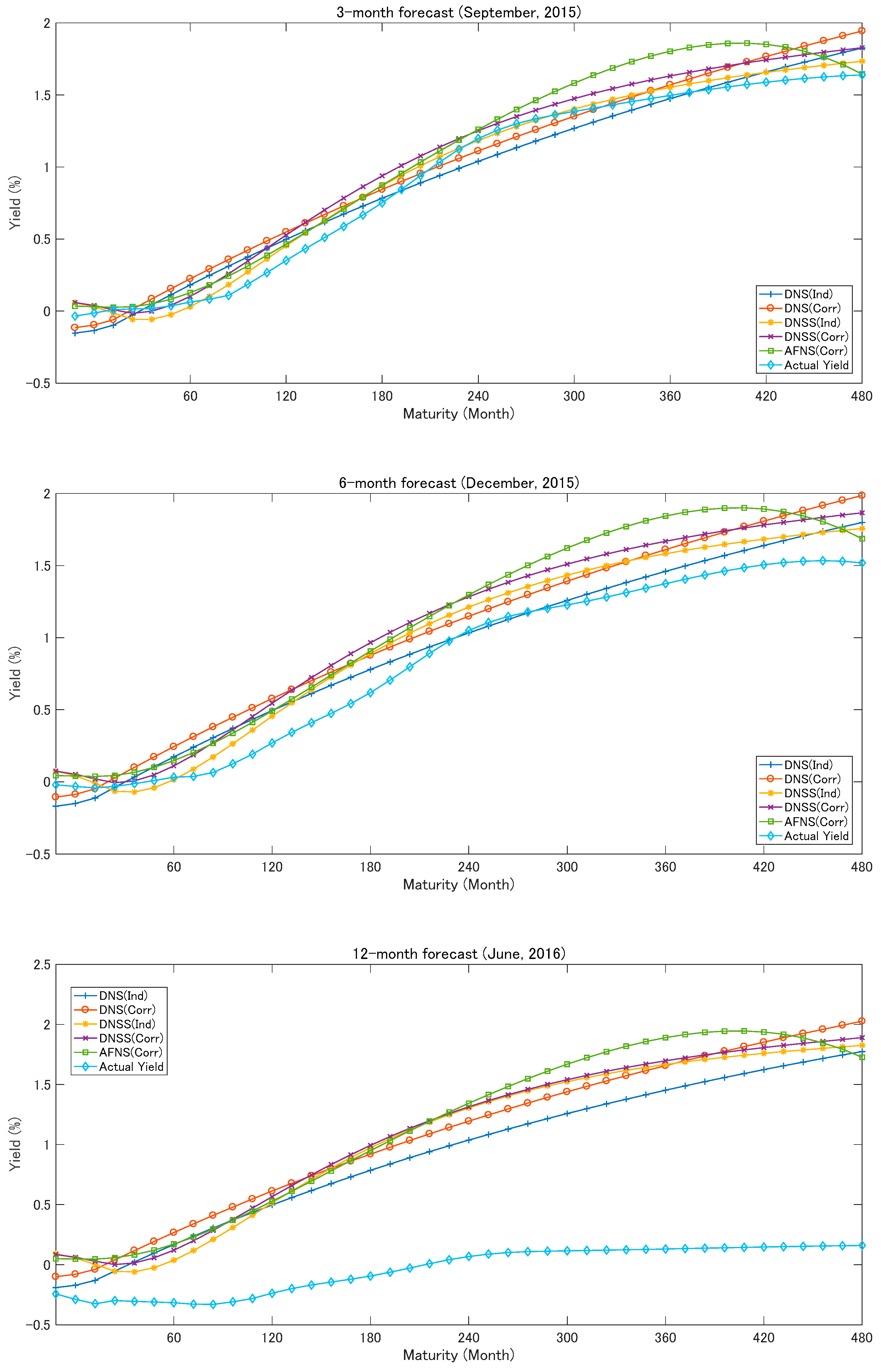
The first plot in Figure 3 depicts the 3-month forecast yields of each model.
Each model captured the actual yield well, as shown by the first and second plots for the 3- and 6-month forecast yields of each model. The forecast performance became poorer as the forecasting horizon becomes longer19.
The correlated AFNS captured the convexity due to the yield adjustment term, while the DNS model and the DNSS model did not capture that effect. We could see a large difference between the two curve-fitting models and the affine term structure model. Moreover, the plot of the DNS model was U-shaped and that of the DNSS model was S-shaped; such a difference in shape between models arose from the fourth term of the DNSS model. The figures suggest that the DNSS model captured the dynamics of the yield more flexibly than the DNS model.
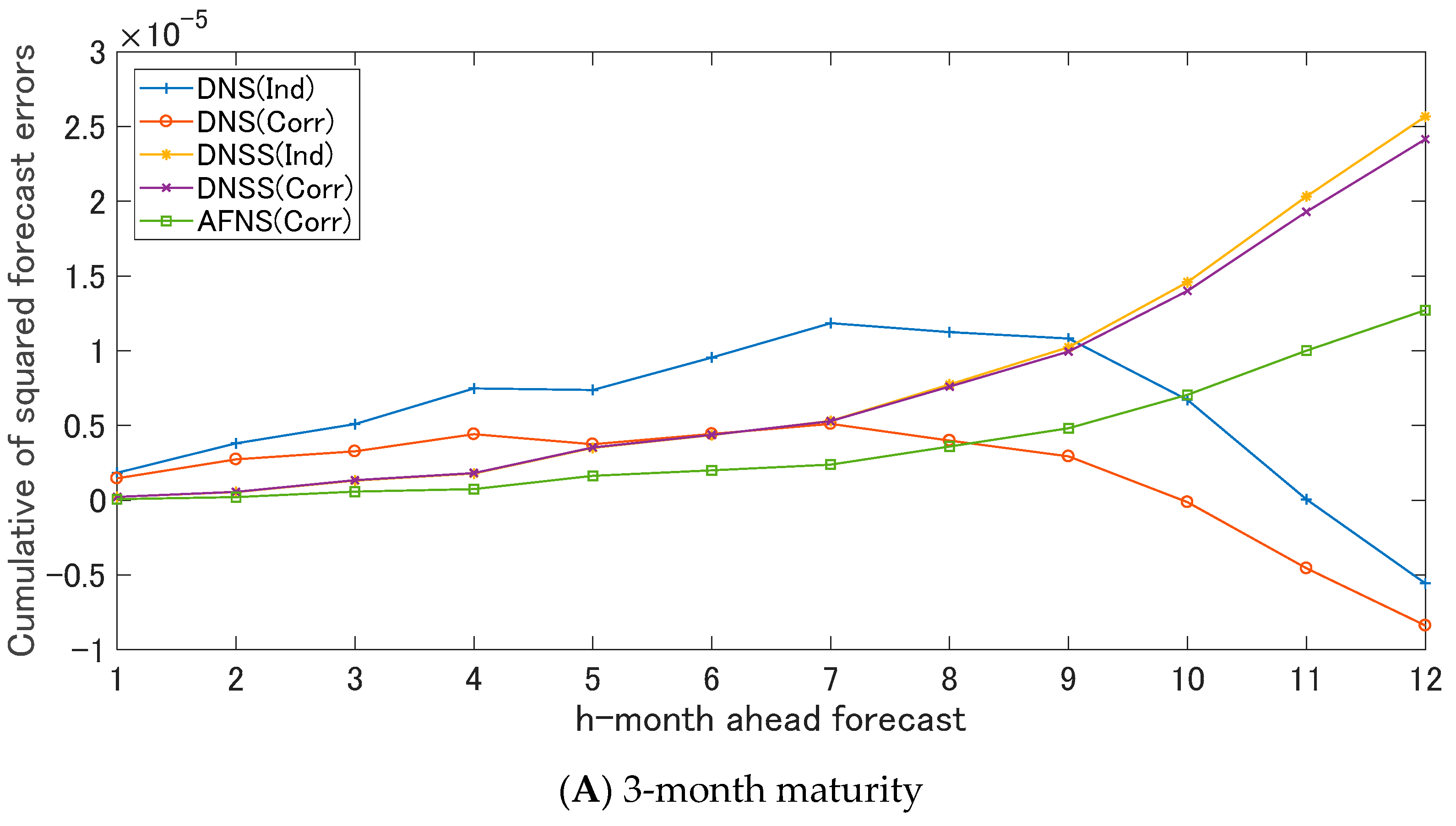
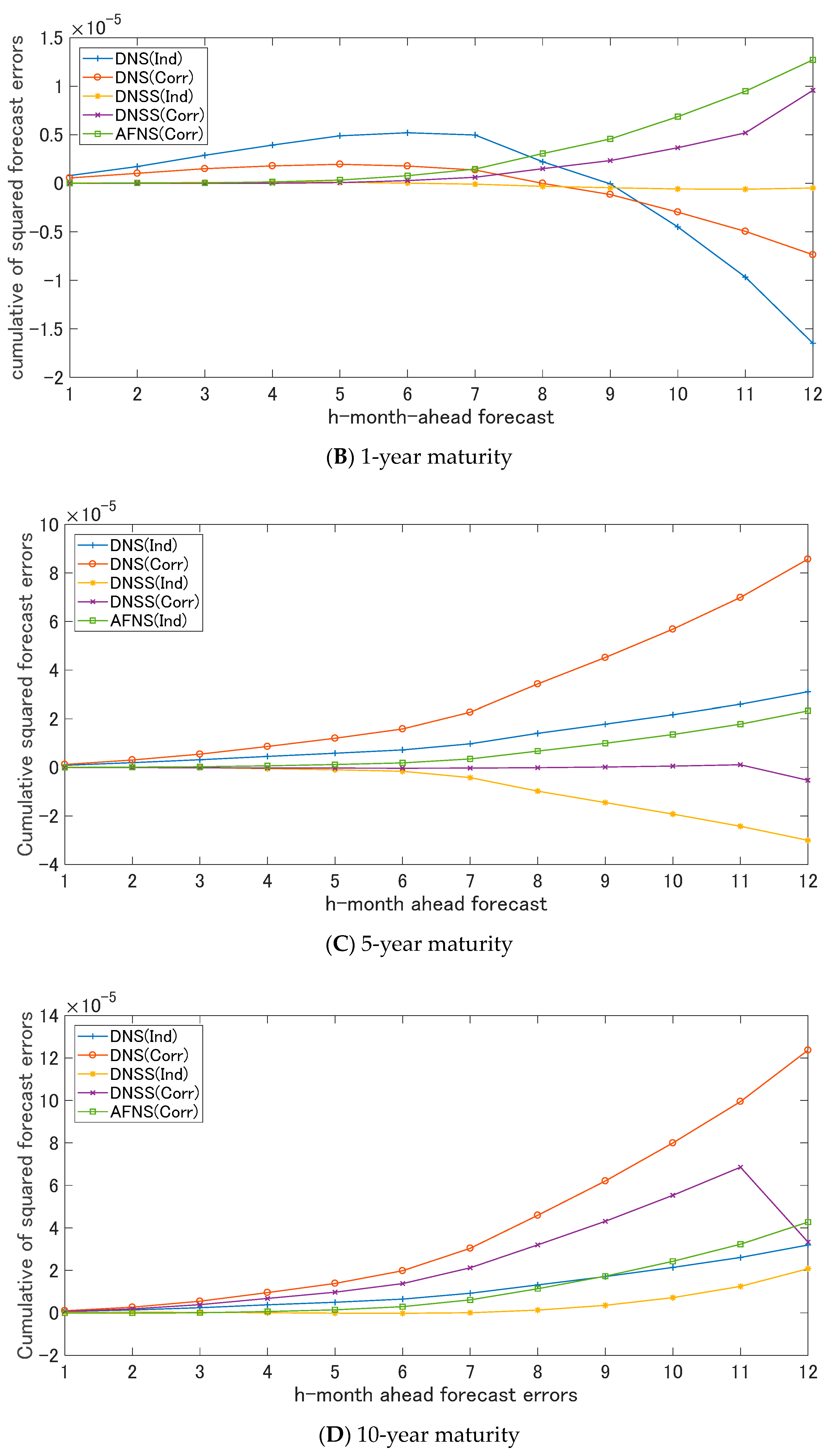
In addition to the above analysis of the forecast accuracy, this paper investigated the cumulative of the squared forecast errors to compare the forecast accuracy of the models with the benchmark model. Figure 4 shows the cumulative of the squared forecast errors of the JGB yields of the 3-month, 1-, 5-, and 10-year maturity. The cumulative of the squared forecast errors imply that the upward (downward) trend in the plot suggest that the models are inferior (superior) to the benchmark model (the random walk model). In the forecasting the JGB yields of 3-month maturity and 1-year maturity, the cumulative of the squared errors of the DNS model shows the downward trend for long-forecast horizon. On the other hand, the cumulative of the squared errors of the DNSS model shows the downward trend for the long forecast horizon. These results provide the evidence that the DNS and the DNSS model is more useful for forecasting the long-term horizon than the random walk model from the perspective of the cumulative of the squared forecast errors.

5.2. Volatility Effect

As the yield adjustment term depends on the volatility matrix, it is often called the volatility effect. In this sub-section, we refer to the yield adjustment term as the volatility effect and discuss it for JGB markets.
Diebold and Rudebusch (2013) argued that the volatility effect can be negligible in most periods, but may become larger in some periods. They also argued that the effect becomes larger with longer maturities.
The volatility effect generated a large difference between the DNS, DNSS, and AFNS models, since it affects the value of the state variables. As discussed in Section 4.1, it caused the constant term bias. The volatility effect arose from the non-linearity of the yield curve. It can be paraphrased mathematically as the Jensen’s inequality term. In the economic literature, it has often been ignored, as a negligible quantity. However, with the exception of in finance research, this concept is typically not discussed at length.
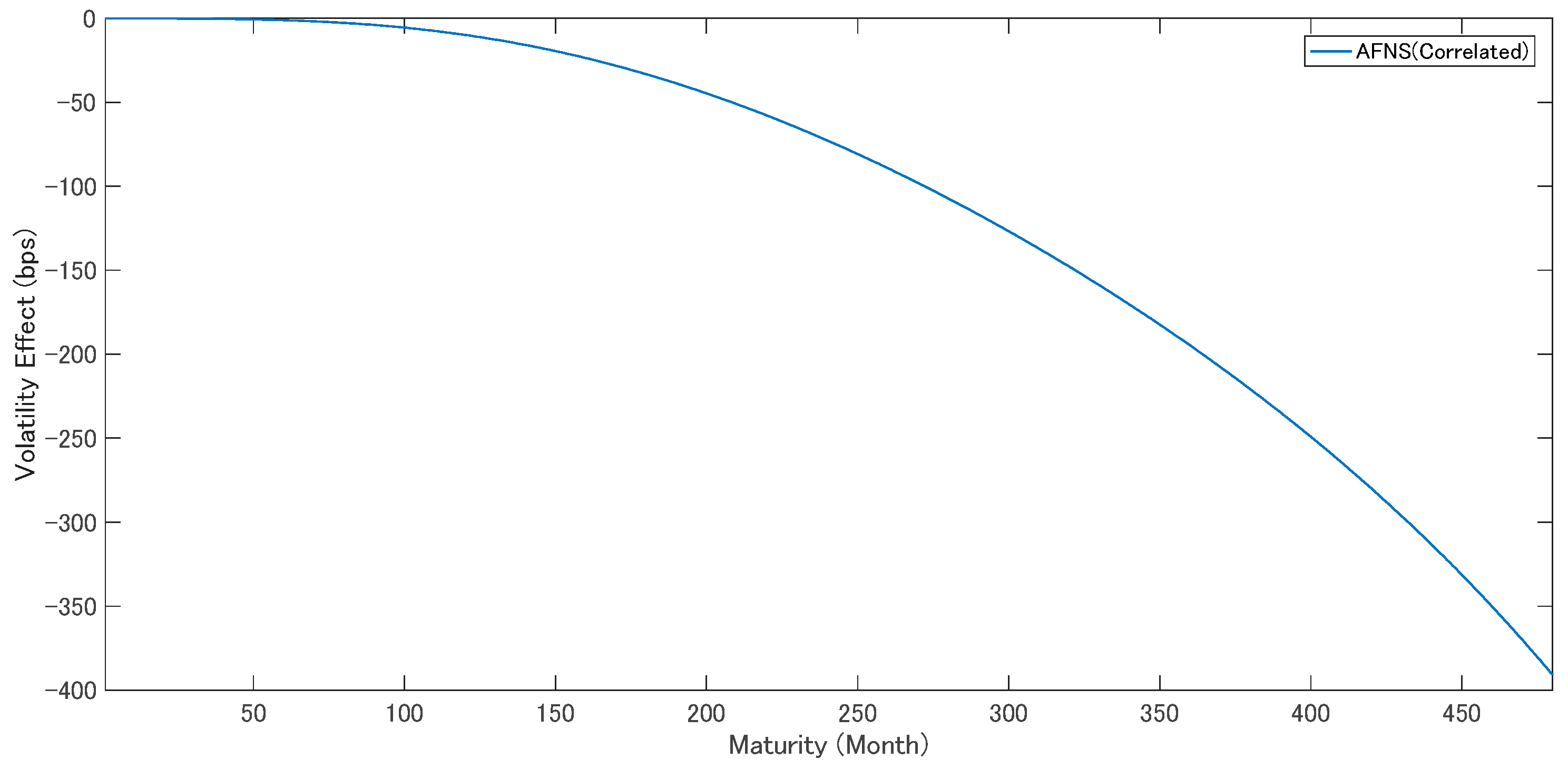
Figure 4 shows the volatility effect, which was calculated20 from the yield adjustment terms of the AFNS model. The volatility effect depended only on maturity, independent of the time. We can confirm that the magnitude of the volatility effect grew larger with longer maturities, in agreement with Diebold and Rudebusch (2013). The magnitude of the volatility effect was 9.8 bp for a 120-month maturity and 126 bp for a 300-month maturity. Hence, we might be able to ignore the effect for maturities from 3- to 120-months, which were practically well used. However, when we are interested in longer-term maturities, such as 300- and 480-month maturities, the volatility effect should be taken into account in the analysis.

6. Conclusions

This study investigated the forecasting performances for yields by the DNS, DNSS, and AFNS models. The DNS and DNSS models are curve-fitting models, which do not impose an arbitrage-free condition. On the other hand, the AFNS model is an affine term structure model based on the arbitrage-free theory.
Following Christensen et al. (2011) and Diebold and Rudebusch (2013), we first introduced the theoretical and empirical framework of the three models. The AFNS was different from the other two models, in that includes a yield adjustment term in the yield curve equation.
Second, our study provided evidence that the DNSS model was the best model, in terms of forecast performance for yields in JGB markets. The forecast performance of the AFNS model was inferior to the DNS model for the 12-month forecast horizon. Our results were in contrast with those of Christensen et al. (2011) and Diebold and Rudebusch (2013), which showed that the AFNS model was superior to the DNS model for U.S. bond data. For JGB markets, the imposition of the arbitrage-free condition did not improve the forecast performance for relatively long forecasting horizons.
The volatility effect was negligibly small for the short maturities. On the other hand, the longer the maturity was, the bigger the volatility effect became. Therefore, when we consider yields at long maturities, we need to pay attention to the existence of the volatility effect.
Finally, we shortly discussed the remaining issues and the directions of future researches. This study adopted the period from August 2009 to June 2015. However, in February 2016, the Bank of Japan carried out the “minus” interest rate policy, which should have created a large, unpredictable shock in the JGB markets. As a large shock generates arbitrage opportunities, the analyses may be biased without taking this into account. Therefore, we need to replicate the analysis over another period.
In this paper, although we used only the three-factor AFNS model, it is also worth using the generalized model of the AFNS model. If so, we may compare the DNSS model with the arbitrage-free Nelson–Siegel model appropriately.

Funding

This research received no external funding.

Conflicts of Interest

The authors declare no conflicts of interest associated with this article.

Appendix A. Derivation of the Theoretical Models

Appendix A.1. Yield of the Nelson–Siegel Model

The forward yield function of the Nelson–Siegel model,
f ( τ ) = β 1 + β 2 e λ τ + β 3 λ τ e λ τ ,
can be described as:
y ( τ ) = β 1 + β 2 ( 1 e λ τ λ τ ) + β 3 ( 1 e λ τ λ τ e λ τ ) .
Proof. 
y ( τ ) = 1 τ 0 τ ( β 1 + β 2 e λ τ + β 3 λ τ e λ τ ) d u = 1 τ { 0 τ β 1 d u + 0 τ β 2 e λ u d u + 0 τ β 3 λ u e λ u d u } = 1 τ { β 1 0 τ 1 d u + β 2 0 τ e λ u d u + β 3 0 τ λ u e λ u d u } = 1 τ { β 1 [ u ] 0 τ + β 2 [ e λ u λ ] 0 τ + β 3 [ u e λ u ] 0 τ + β 3 0 τ e λ u d u } = 1 τ { β 3 τ + β 2 1 e λ τ λ β 3 τ e λ τ + β 3 [ e λ u λ ] 0 τ } = 1 τ { β 1 τ + β 2 1 e λ τ λ β 3 τ e λ τ + β 3 1 e λ τ λ } = β 1 + β 2 ( 1 e λ τ λ τ ) + β 3 ( 1 e λ τ λ τ e λ τ ) .
 □

Appendix A.2. Yield of the Nelson–Siegel–Svensson Model

The forward yield function of the Nelson–Siegel–Svensson model,
f ( τ ) = β 1 + β 2 e λ 1 τ + β 3 λ 1 τ e λ 1 τ + β 4 λ 2 τ e λ 2 τ ,
can be described as:
y ( τ ) = β 1 + β 2 ( 1 e λ 1 τ λ 1 τ ) + β 3 ( 1 e λ 1 τ λ 1 τ e λ 1 τ ) + β 4 ( 1 e λ 2 τ λ 2 τ e λ 2 τ ) .
Proof. 
y ( τ ) = 1 τ 0 τ { β 1 + β 2 e λ 1 s + β 3 λ 1 s e λ 1 s + β 4 λ 2 s e λ 2 s } d s = 1 τ { 0 τ β 1 d s + 0 τ β 2 e λ 1 s d s + 0 τ β 3 λ 1 s e λ 1 s d s + 0 τ β 4 λ 2 s e λ 2 s d s } = 1 τ { [ β 1 s ] 0 τ + β 2 [ e λ 1 s λ 1 ] 0 τ + β 3 ( τ e λ 1 τ + 0 τ e λ 1 s d s )       + β 4 ( τ e λ 2 τ + 0 τ e λ 2 s d s ) } = 1 τ { β 1 τ + β 2 ( 1 e λ 1 τ λ 1 ) + β 3 ( τ e λ 1 τ + [ e λ 1 τ λ 1 ] 0 τ )       + β 4 ( τ e λ 2 τ + [ e λ 2 τ λ 2 ] 0 τ ) } = 1 τ { β 1 τ + β 2 ( 1 e λ 1 τ λ 1 ) + β 3 ( 1 e λ 1 τ λ 1 τ e λ 1 τ ) + β 4 ( 1 e λ 2 τ λ 2 τ e λ 2 τ ) } = β 1 + β 2 ( 1 e λ 1 τ λ 1 τ ) + β 3 ( 1 e λ 1 τ λ 1 τ e λ 1 τ ) + β 4 ( 1 e λ 2 τ λ 2 τ e λ 2 τ ) .
 □

Appendix A.3. Affine Term Structure Model of Duffie and Kan

We considered the Duffie–Kan framework (Duffie and Kan (1996)) for defining the arbitrage-free Nelson–Siegel model. By substituting the Nelson–Siegel factors into the state variable of the Duffie–Kan framework, we can make the Nelson–Siegel model arbitrage-free.
In Duffie and Kan, the filtered probability space is ( Ω , t , Q ) , where the filtration is:
t = { t , t 0 } ,
and the state variables are X t on a set M n , which is a Markov process and the solution of the stochastic differential equation,
d X ( t ) = κ ( t ) ( θ ( t ) X ( t ) ) d t + Σ ( t ) D ( X t , t ) d W ( t ) ,
where W is the standard Brownian motion in n .
In Duffie and Kan (1996), the definition of D ( X t , t ) is:
D ( X t , t ) = [ γ 1 ( t ) + δ 1 ( t ) X t 0 0 γ n ( t ) + δ n ( t ) X t ] ,
which is a diagonal matrix where δ i ( t ) denotes the i th row of the matrix:
δ i ( t ) = [ δ 1 1 ( t ) δ n 1 ( t ) δ 1 n ( t ) δ n n ( t ) ] .
The instantaneous risk-free rate is represented by an affine function; that is,
r t = ρ 0 ( t ) + ρ 1 ( t ) X t ,
where each parameter is bounded and continuous, respectively; that is, θ : [ 0 , T ] n , κ : [ 0 , T ] n × n ,   Σ : [ 0 , T ] n × n ,   D : M × [ 0 , T ] n × n ,   γ : [ 0 , T ] n × n ,   δ : [ 0 , T ] n × n ,   ρ 0 : [ 0 , T ] ,   ρ 1 : [ 0 , T ] n .
Proposition A1.
The zero-coupon price is represented as
P ( t , T ) = E t [ e t T r u d u ] = e B ( t , T ) X t + C ( t , T ) ,
under the above assumptions, where B ( t , T ) and C ( t , T ) are the solutions of following ordinary differential equation systems under the boundary conditions B ( T , T ) = 0   a n d   C ( T , T ) = 0 ,
d B ( t , T ) d t = ρ 1 + ( κ ) B ( t , T ) 1 2 j = 1 n ( Σ B ( t , T ) B ( t , T ) Σ ) j , j ( δ j ) ,
d C ( t , T ) d t = ρ 0 B ( t , T ) κ θ 1 2 j = 1 n ( Σ B ( t , T ) B ( t , T ) Σ ) j , j γ j .
Then, the yield is given by:
Y ( t , T ) = 1 T t log P ( t , T ) = B ( t , T ) T t X t C ( t , T ) T t .
Proof. 
 
Here, we consider three factors (or three state variables).
The bond price is described as:
P t ( τ ) = E t [ e t T r u d u ] .
From the Feynman–Kac formula, we can describe the bond price as:
P t ( τ ) = F ( X t , τ ) ,
where F ( x t , τ ) solves the partial differential equation:
F ( X ( t ) , τ ) r ( t ) = F ( X ( t ) , τ ) τ + i = 1 3 [ F ( X ( t ) , τ ) x i κ ( t ) ( θ ( t ) X ( t ) ) + 1 2 2 F ( X ( t ) , τ ) x i 2 Σ D ( X ( t ) , t ) D ( X ( t ) , t ) Σ ] ,
and we can write it as:
F ( X ( t ) , τ ) = e B ( t , T ) X t + C ( t , T ) .
From this equation, the first differential of X i   and   τ , and the second differential of X i are given by:
F ( X ( t ) , τ ) x i = B ( t , T ) F ( X ( t ) , τ ) ,
F ( X ( t ) , τ ) x i 2 = B ( t , T ) B ( t , T ) F ( X ( t ) , τ ) ,
F ( X ( t ) , τ ) τ = [ B ( t , T ) x t + C ( t , T ) ] F ( X ( t ) , τ ) .
Substituting these equations into the Equation (A16), we obtain:
F ( X ( t ) , τ ) r ( t ) = F ( X ( t ) , τ ) τ          + i = 1 3 [ F ( X ( t ) , τ ) x i κ ( t ) ( θ ( t ) X ( t ) )          + 1 2 2 F ( X ( t ) , τ ) x i 2 Σ D ( X ( t ) , t ) D ( X ( t ) , t ) Σ ] = [ B ( t , T ) X t + C ( t , T ) ] F ( X ( t ) , τ ) + i = 1 3 [ B ( t , T ) F ( X ( t ) , τ ) κ ( t ) ( θ ( t ) X ( t ) ) + 1 2 F ( X ( t ) , τ ) ( Σ B ( t , T ) B ( t , T ) Σ ) j , j D ( X ( t ) , t ) D ( X ( t ) , t ) ] .
From the definition of the matrix D ( X ( t ) , t ) ,
r ( t ) = [ B ( t , T ) X t + C ( t , T ) ]          + i = 1 3 [ B ( t , T ) κ ( t ) ( θ ( t ) X ( t ) )          + 1 2 ( Σ B ( t , T ) B ( t , T ) Σ ) j , j ( γ j ( t ) + δ j ( t ) X t ) ] = [ B ( t , T ) X t + C ( t , T ) ]          + i = 1 3 [ B ( t , T ) κ ( t ) ( θ ( t ) X ( t ) )          + 1 2 ( Σ B ( t , T ) B ( t , T ) Σ ) j , j ( γ j ( t ) )          + 1 2 ( Σ B ( t , T ) B ( t , T ) Σ ) j , j ( δ j ( t ) X t ) ] = [ B ( t , T ) d t B ( t , T ) κ ( t ) + 1 2 i = 1 3 ( Σ B ( t , T ) B ( t , T ) Σ ) j , j δ j ( t ) ] X t + [ C ( t , T ) d t +    B ( t , T ) κ ( t ) θ ( t ) + 1 2 i = 1 3 ( Σ B ( t , T ) B ( t , T ) Σ ) j , j ( γ j ( t ) ) ] .
From the definition of r t = ρ 0 ( t ) + ρ 1 ( t ) X t , we obtain:
ρ 1 ( t ) = B ( t , T ) d t B ( t , T ) κ ( t ) + 1 2 i = 1 3 ( Σ B ( t , T ) B ( t , T ) Σ ) j , j δ j ( t ) ,
ρ 0 ( t ) = C ( t , T ) d t + B ( t , T ) κ ( t ) θ ( t ) + 1 2 i = 1 3 ( Σ B ( t , T ) B ( t , T ) Σ ) j , j ( γ j ( t ) ) .
Arranging the equations, we get:
B ( t , T ) d t = ρ 1 ( t ) + B ( t , T ) κ ( t ) 1 2 i = 1 3 ( Σ B ( t , T ) B ( t , T ) Σ ) j , j δ j ( t ) ,
C ( t , T ) d t = ρ 0 ( t ) B ( t , T ) κ ( t ) θ ( t ) 1 2 i = 1 3 ( Σ B ( t , T ) B ( t , T ) Σ ) j , j ( γ j ( t ) ) ,
where boundary condition is:
B ( T , T ) = C ( T , T ) = 0 .
Then, the solutions of the ordinary differential equations are B ( t , T ) , C ( t , T ) , and the yield functions:
Y ( t , T ) = 1 T t log P ( t , T ) = B ( t , T ) T t X t C ( t , T ) T t .
 □

Appendix A.4. Arbitrage-Free Nelson–Siegel Model

In this appendix, we show the derivation of the arbitrage-free Nelson–Siegel model following Christensen et al. (2011).
We use Equation (24) from the main text:
d B ( t , T ) d t = ρ 1 + ( κ ) B ( t , T ) ,
and the relationship as follows,
d d t [ e ( κ ) ( T t ) B ( t , T ) ] = e ( κ ) ( T t ) d B ( t , T ) d t e ( κ ) ( T t ) ( κ ) B ( t , T ) .
Substituting the Equation (A26) into the Equation (A27), we obtain:
d d t [ e ( κ ) ( T t ) B ( t , T ) ]        = ρ 1 e ( κ ) ( T t ) + e ( κ ) ( T t ) ( κ ) B ( t , T ) e ( κ ) ( T t ) ( κ ) B ( t , T )        = ρ 1 e ( κ ) ( T t ) .
The integration of the Equation (A28) is written as:
t T d d s [ e ( κ ) ( T s ) B ( s , T ) ] d s = t T ρ 1 e ( κ ) ( T s ) d s . t T d [ e ( κ ) ( T s ) B ( s , T ) ] = t T ρ 1 e ( κ ) ( T s ) d s .          [ e ( κ ) ( T s ) B ( s , T ) ] t T = t T ρ 1 e ( κ ) ( T s ) d s .
From the boundary condition B ( T , T ) = 0 , the Equation (A29) can be rewritten as:
B ( t , T ) = e ( κ ) ( T t ) t T ρ 1 e ( κ ) ( T s ) d s .
From the restrictions (30), (31), and (32) in the main text, we obtain:
B ( t , T ) = [ ( T t ) 1 e λ ( T t ) λ ( T t ) e λ ( T t ) 1 e λ ( T t ) λ ] .

Appendix A.5. Yield Adjustment Term of Arbitrage-Free Nelson–Siegel Model

In this appendix, we show the derivation of the yield adjustment the arbitrage-free Nelson–Siegel model following Christensen et al. (2011).
Proposition A2.
Fixing the average levels of state variables, which, under measure, we can identify the yield adjustment term of the three-factor arbitrage-free Nelson–Siegel model.
Under the Q measure, θ = 0 , and so we can represent the yield adjustment term C ( t , T ) as:
C ( t , T ) T t = 1 2 1 T t j = 1 3 t T ( Σ B ( s , T ) B ( s , T ) Σ ) j , j d s .
Then, we can write above equation as:
C ( t , T ) T t = A ¯ ( ( T t ) 2 6 ) + B ¯ ( 1 2 λ 2 1 λ 3 1 e λ ( T t ) T t + 1 4 λ 3 1 e 2 λ ( T t ) T t ) + C ¯ ( 1 2 λ 2 + 1 λ 2 e λ ( T t ) 1 4 λ ( T t ) e 2 λ ( T t ) 3 4 λ 2 e 2 λ ( T t ) 2 λ 3 1 e λ ( T t ) T t + 5 8 λ 3 1 e 2 λ ( T t ) T t ) + D ¯ ( 1 2 λ ( T t ) + 1 λ 2 e λ ( T t ) 1 λ 3 1 e λ ( T t ) T t ) + E ¯ ( 3 λ 2 e λ ( T t ) + 1 2 λ ( T t ) + 1 λ ( T t ) e λ ( T t ) 3 λ 3 1 e λ ( T t ) T t + F ¯ ( 1 λ 2 + 1 λ 2 e λ ( T t ) 1 2 λ 2 e 2 λ ( T t ) 3 λ 3 1 e λ ( T t ) T t + 3 4 λ 3 1 e λ ( T t ) T t ) ,
where:
Σ = [ σ 11 σ 12 σ 13 σ 21 σ 22 σ 23 σ 31 σ 32 σ 33 ] ,
and:
A ¯ = σ 11 2 + σ 12 2 + σ 13 2 ,
B ¯ = σ 21 2 + σ 22 2 + σ 23 2 ,
C ¯ = σ 31 2 + σ 32 2 + σ 33 2 ,
D ¯ = σ 11 σ 21 + σ 12 σ 22 + σ 13 σ 23 ,
E ¯ = σ 11 σ 31 + σ 12 σ 32 + σ 13 σ 33 ,   and
F ¯ = σ 21 σ 31 + σ 22 σ 32 + σ 23 σ 33 .
Proof. 
C ( t , T ) T t = 1 2 1 T t j = 1 3 t T ( Σ B ( S , T ) B ( S , T ) Σ ) j , j d s         = A ¯ 2 1 T t t T B 1 ( S , T ) 2 d s + B ¯ 2 1 T t t T B 2 ( S , T ) 2 d s         + C ¯ 2 1 T t t T B 3 ( S , T ) 2 d s + D ¯ 2 1 T t t T B 1 ( S , T ) B 2 ( S , T ) d s         + D ¯ 2 1 T t t T B 2 ( S , T ) B 1 ( S , T ) d s + E ¯ 2 1 T t t T B 1 ( S , T ) B 3 ( S , T ) d s         + E ¯ 2 1 T t t T B 3 ( S , T ) B 1 ( S , T ) d s + F ¯ 2 1 T t t T B 2 ( S , T ) B 3 ( S , T ) d s         + F ¯ 2 1 T t t T B 3 ( S , T ) B 2 ( S , T ) d s = A ¯ 2 1 T t t T B 1 ( S , T ) 2 d s + B ¯ 2 1 T t t T B 2 ( S , T ) 2 d s + C ¯ 2 1 T t t T B 3 ( S , T ) 2 d s +    D ¯ T t t T B 1 ( S , T ) B 2 ( S , T ) d s + F ¯ T t t T B 1 ( S , T ) B 3 ( S , T ) d s a 34 +            F ¯ T t t T B 2 ( S , T ) B 3 ( S , T ) d s ,
where:
A ¯ = σ 11 2 + σ 12 2 + σ 13 2 ,
B ¯ = σ 21 2 + σ 22 2 + σ 23 2 ,
C ¯ = σ 31 2 + σ 32 2 + σ 33 2 ,
D ¯ = σ 11 σ 21 + σ 12 σ 22 + σ 13 σ 23 ,
E ¯ = σ 11 σ 31 + σ 12 σ 32 + σ 13 σ 33 ,   and
F ¯ = σ 21 σ 31 + σ 22 σ 32 + σ 23 σ 33 .
We define each term of Equation (A34) as:
I A A ¯ 2 1 T t t T B 1 ( s , T ) 2 d s ,
I B B ¯ 2 1 T t t T B 2 ( s , T ) 2 d s ,
I C C ¯ 2 1 T t t T B 3 ( s , T ) 2 d s ,
I D D ¯ T t t T B 1 ( s , T ) B 2 ( s , T ) d s ,
I E E ¯ T t t T B 1 ( s , T ) B 3 ( s , T ) d s ,   and
I F F ¯ T t t T B 2 ( s , T ) B 3 ( s , T ) d s ,
respectively.
From the previous section,
B 1 ( t , T ) = ( T t ) ,
B 2 ( t , T ) = 1 e λ ( T t ) λ ,   and
B 3 ( t , T ) = ( T t ) e λ ( T t ) 1 e λ ( T t ) λ .
Substituting these into Equations (A35)–(A40), we can derive the analytical forms:
I A = A ¯ 2 1 T t t T B 1 ( s , T ) 2 d s = A ¯ 2 1 T t t T ( T s ) 2 d s = A ¯ 2 1 T t [ ( T s ) 3 3 ] t T = A ¯ 2 1 T t ( T t ) 3 3 = A ¯ 6 ( T t ) 2 ,
I B = B ¯ 2 1 T t t T B 2 ( s , T ) 2 d s = B ¯ 2 1 T t t T [ 1 e λ ( T s ) λ ] 2 d s         = B ¯ 2 1 T t t T [ 1 2 e λ ( T s ) + e 2 λ ( T s ) λ 2 ] d s = B ¯ 2 1 T t { t T 1 λ 2 d s t T 2 e λ ( T s ) λ 2 d s + t T e 2 λ ( T s ) λ 2 d s }         = B ¯ 2 1 T t { [ s λ 2 ] t T [ 2 e λ ( T s ) λ 3 ] t T + [ [ e 2 λ ( T s ) 2 λ 3 ] t T ] } = B ¯ 2 1 T t { T t λ 2 2 2 e λ ( T t ) λ 3 + 1 e 2 λ ( T t ) 2 λ 3 } = B ¯ { 1 2 λ 2 1 λ 3 1 e λ ( T t ) T t + 1 4 λ 3 1 e 2 λ ( T t ) T t } ,
I C = C ¯ 2 1 T t t T B 3 ( s , T ) 2 d s = C ¯ 2 1 T t [ t T ( T s ) 2 e 2 λ ( T s ) d s t T 2 ( T s ) e λ ( T s ) λ d s        + t T 2 ( T s ) e 2 λ ( T s ) λ d s + t T 1 λ 2 d s t T 2 e λ ( T s ) λ 2 d s        + t T e 2 λ ( T s ) λ 2 d s ] = C ¯ 2 1 T t { [ ( T s ) 2 ( e 2 λ ( T s ) 2 λ ) ] t T t T 2 ( T s ) e 2 λ ( T s ) 2 λ d s        1 λ { [ 2 ( T s ) ( e λ ( T s ) λ ) ] t T t T 2 e 2 λ ( T s ) 2 λ d s } + [ s λ 2 ] t T [ 2 e λ ( T s ) λ 3 ] t T        + [ e 2 λ ( T s ) 2 λ 3 ] t T } = C ¯ 2 1 T t { ( T t ) 2 e 2 λ ( T t ) 2 λ 2 ( T t ) e 2 λ ( T t ) 4 λ 2 + t T e 2 λ ( T s ) 4 λ 2 d s        + 1 λ { 2 ( T t ) e λ ( T t ) λ [ 2 e λ ( T t ) λ 2 ] t T }        1 λ { 2 ( T t ) e 2 λ ( T s ) 2 λ [ e 2 λ ( T t ) 2 λ 2 ] } + T t λ 2 2 2 e λ ( T t ) λ 3        + 1 1 e 2 λ ( T t ) 2 λ 3 } = C ¯ 2 1 T t { ( T t ) 2 e 2 λ ( T t ) 2 λ ( T t ) e 2 λ ( T t ) 2 λ 2 1 e 2 λ ( T t ) 4 λ 3 + 2 e λ ( T t ) λ 2 ( T t )        2 2 e λ ( T t ) λ 3 e 2 λ ( T t ) λ 2 ( T t ) + 1 e 2 λ ( T t ) 2 λ 3 + T t λ 2        2 2 e λ ( T t ) λ 3 + 1 1 e 2 λ ( T t ) 2 λ 3 } = C ¯ 2 1 T t { ( T t ) 2 e 2 λ ( T t ) 2 λ ( T t ) e 2 λ ( T t ) 2 λ 2 1 e 2 λ ( T t ) 4 λ 3 + 2 e λ ( T t ) λ 2 ( T t )        2 2 e λ ( T t ) λ 3 e 2 λ ( T t ) λ 2 ( T t ) + 1 e 2 λ ( T t ) 2 λ 3 + T t λ 2        2 2 e λ ( T t ) λ 3 + 1 1 e 2 λ ( T t ) 2 λ 3 } = C ¯ { e 2 λ ( T t ) 4 λ ( T t ) e 2 λ ( T t ) 4 λ 2 + 1 8 λ 3 1 e 2 λ ( T t ) T t + e λ ( T t ) λ 2 1 λ 3 1 e λ ( T t ) T t        e 2 λ ( T t ) 2 λ 2 + 4 λ 3 1 e 2 λ ( T t ) T t + 1 2 λ 2 1 λ 3 1 e λ ( T t ) T t        + 1 4 λ 3 1 e 2 λ ( T t ) T t } = C ¯ { 1 2 λ 2 + e λ ( T t ) λ 2 e 2 λ ( T t ) 2 λ 2 e 2 λ ( T t ) 4 λ ( T t ) e 2 λ ( T t ) 4 λ 2 e 2 λ ( T t ) 2 λ 2        1 λ 3 1 e λ ( T t ) T t 1 λ 3 1 e λ ( T t ) T t + 1 8 λ 3 1 e 2 λ ( T t ) T t         + 2 4 λ 3 1 e 2 λ ( T t ) T t } = C ¯ { 1 2 λ 2 + e λ ( T t ) 2 λ 2 e 2 λ ( T t ) 4 λ ( T t ) 3 4 λ 2 e 2 λ ( T t ) 2 λ 3 1 e λ ( T t ) T t + 5 8 λ 3 1 e 2 λ ( T t ) T t } ,
I D = D ¯ T t t T B 1 ( s , T ) B 2 ( s , T ) d s = D ¯ T t t T [ ( T s ) ] [ 1 e λ ( T s ) λ ] d s         = D ¯ T t t T ( T s ) ( T s ) e λ ( T s ) λ d s         = D ¯ T t { t T ( T s ) λ d s t T ( T s ) e λ ( T s ) λ d s }         = D ¯ T t { [ ( T s ) 2 2 λ ] t T [ ( T s ) e λ ( T s ) λ 2 ] t T t T e λ ( T s ) λ 2 d s }         = D ¯ T t { ( T t ) 2 2 λ + e λ ( T s ) λ 2 ( T t ) [ e λ ( T s ) λ 3 ] t T }         = D ¯ T t { ( T t ) 2 2 λ + e λ ( T s ) λ 2 ( T t ) 1 e λ ( T s ) λ 3 }         = D ¯ { T t 2 λ + 1 λ 2 e λ ( T t ) 1 λ 3 1 e λ ( T t ) T t } ,
I E = E ¯ T t t T B 1 ( s , T ) B 3 ( s , T ) d s = E ¯ T t { t T [ ( T s ) ] [ ( T s ) e λ ( T s ) 1 e λ ( T s ) λ ] d s } = E ¯ T t { t T ( T s ) 2 e λ ( T s ) d s + t T ( T s ) ( T s ) e λ ( T s ) λ d s } = E ¯ T t { [ ( T s ) 2 e λ ( T s ) λ ] t T          t T 2 ( T s ) e λ ( T s ) λ d s + t T T s λ d s t T ( T s ) e λ ( T s ) λ d s } = E ¯ T t { ( T t ) 2 e λ ( T t ) λ [ 2 ( T s ) e λ ( T s ) λ 2 ] t T          t T 2 e λ ( T s ) λ 2 d s [ ( T s ) 2 2 λ ] t T [ ( T s ) e λ ( T s ) λ 2 ] t T t T e λ ( T s ) λ 2 d s } = E ¯ T t { ( T t ) 2 e λ ( T t ) λ + 2 ( T t ) e λ ( T t ) λ 2 [ 2 e λ ( T s ) λ 3 ] t T + ( T t ) 2 2 λ          [ ( T t ) e λ ( T s ) λ 2 ] t T [ e λ ( T s ) λ 3 ] t T } = E ¯ T t { ( T t ) 2 e λ ( T t ) λ + 2 ( T t ) e λ ( T t ) λ 2 2 2 e λ ( T s ) λ 3 + ( T t ) 2 2 λ          + ( T t ) e λ ( T t ) λ 2 1 e λ ( T s ) λ 3 }      = E ¯ { e λ ( T t ) λ ( T t ) e λ ( T t ) + 3 λ 2 e λ ( T t ) + T t 2 λ 3 λ 3 1 1 e λ ( T s ) T t } ,   and
I F = F ¯ T t t T B 2 ( s , T ) B 3 ( s , T ) d s = F ¯ T t { t T ( T s ) e λ ( T s ) λ d s + t T ( T s ) e 2 λ ( T s ) λ d s + t T 1 λ 2 d s        t T 2 e λ ( T s ) λ 2 d s + t T e 2 λ ( T s ) λ 2 d s } = F ¯ T t { [ ( T s ) e λ ( T s ) λ 2 ] t T t T e λ ( T s ) λ 2 d s + [ ( T s ) e 2 λ ( T s ) 2 λ 2 ] t T + t T e 2 λ ( T s ) 2 λ 2 d s          + [ s λ 2 ] t T [ 2 e λ ( T s ) λ 3 ] t T + [ e 2 λ ( T s ) λ 2 ] t T } = F ¯ T t { ( T t ) e λ ( T t ) λ 2 [ e λ ( T s ) λ 3 ] t T ( T t ) e 2 λ ( T t ) 2 λ 2 + [ e 2 λ ( T s ) 4 λ 3 ] t T + T t λ 2          2 2 e λ ( T t ) λ 3 + 1 e λ ( T t ) 2 λ 3 } = F ¯ T t { ( T t ) e λ ( T t ) λ 2 1 e λ ( T t ) λ 3 ( T t ) e 2 λ ( T t ) 2 λ 2 + 1 e 2 λ ( T t ) 4 λ 3 + T t λ 2          2 2 e λ ( T t ) λ 3 + 1 e λ ( T t ) 2 λ 3 }        = F ¯ { 1 λ 2 + 1 λ 2 e λ ( T t ) 1 2 λ 2 e 2 λ ( T t ) 3 λ 3 1 e λ ( T t ) T t + 3 4 λ 3 1 e 2 λ ( T t ) T t } .
 □

References

  1. Alfaro, Rodrigo A. 2011. Affine Nelson-Siegel model. Economics Letters 110: 1–3. [Google Scholar] [CrossRef]
  2. Al-Zoubi, Haitham A. 2009. Short-term spot rate models with nonparametric deterministic drift. Quarterly Review of Economics and Finance 49: 731–47. [Google Scholar] [CrossRef]
  3. Ang, Andrew, and Monika Piazzesi. 2003. A no-arbitrage vector autoregression of term structure dynamics with macroeconomi and latent variables. Journal of Monetary Economics 50: 745–87. [Google Scholar] [CrossRef]
  4. Bjork, Tomas, and Bent Jesper Christensen. 1999. Interest rate dynamics and consistent forward rate curves. Mathematical Finance 9: 323–48. [Google Scholar] [CrossRef]
  5. Chan, Ka-keung Ceajer, Andrew Karolyi, Francis A. Longstaff, and Anthony B. Sanders. 1992. An empirical comparison of alternative models of the short-term interest rate. Journal of Finance 47: 1209–27. [Google Scholar] [CrossRef]
  6. Chen, Yu-chin, and Kwok Ping Tsang. 2013. What does the yield curve tell us about exchange rate predictability? Review of Economics and Statistics 95: 185–205. [Google Scholar] [CrossRef]
  7. Christensen, Jens H. E., Francis X. Diebold, and Glenn D. Rudebusch. 2009. An arbitrage-free generalized Nelson-Siegel term structure model. Econometrics Journal 12: C33–C64. [Google Scholar] [CrossRef]
  8. Christensen, Jens H.E., Francis X. Diebold, and Glenn D. Rudebusch. 2011. The affine arbitrage-free class of Nelson-Siegel term structure models. Journal of Econometrics 164: 4–20. [Google Scholar] [CrossRef]
  9. Coroneo, Laura, Ken Nyholm, and Rositsa Vidova-Koleva. 2011. How arbitrage-free is the Nelson-Siegel model? Journal of Empirical Finance 18: 393–407. [Google Scholar] [CrossRef]
  10. Cox, John, Jonathan E. Ingersol, and Stephen A. Ross. 1985. A theory of the term structure of interest rates. Econometrica 53: 385–407. [Google Scholar] [CrossRef]
  11. De Rezende, Rafael B., and Mauro S. Ferreira. 2013. Modeling and forecasting the yield curve by an extended Nelson-Siegel class of models: A quantile autoregression approach. Journal of Forecasting 32: 111–23. [Google Scholar] [CrossRef]
  12. Diebold, Francis X., and Canlin Li. 2006. Forecasting the term structure of government bond yields. Journal of Econometrics 130: 337–64. [Google Scholar] [CrossRef]
  13. Diebold, Francis X., and Robert S. Mariano. 1995. Comparing predictive accuracy. Journal of Business and Economic Statistics 13: 134–44. [Google Scholar]
  14. Diebold, Francis X., and Glenn D. Rudebusch. 2013. Yield Curve Modeling and Forecasting. Princeton: Princeton University Press. [Google Scholar]
  15. Duffee, Gregory R. 2002. Term premia and interest rate forecasts in affine models. Journal of Finance 57: 405–43. [Google Scholar] [CrossRef]
  16. Duffie, Darrell, and Rui Kan. 1996. A yield-factor model of interest rates. Mathematical Finance 6: 379–406. [Google Scholar] [CrossRef]
  17. Fama, Eugene F. 2006. The behavior of interest rates. Review of Financial Studies 19: 359–79. [Google Scholar] [CrossRef]
  18. Fujii, Mariko, and Makoto Takaoka. 2007. Kinri no Kikannkozo to Macrokeizai: Nelson—Siegel Moderu wo Motiita Approach [Term Structure of Interest Rates and Macroeconomy: Nelson—Siegel Model Approach]. FSA Research Review. Tokyo: Financial Services Agency, pp. 219–48. [Google Scholar]
  19. Gasha, Giancarlo, Ying He, Carlos Medeiros, Marco Rodriguez, Jean Salvati, and Jiangbo Yi. 2010. On the Estimation of Term Structure Models and an Application to the United State. IMF Working Paper WP/10/258. Washington: International Monetary Fund. [Google Scholar]
  20. Gurkaynak, Refet S., Brian Sack, and Jonathan H. Wright. 2007. The U.S. treasury yield curve: 1961 to the present. Journal of Monetary Economics 54: 2291–304. [Google Scholar] [CrossRef]
  21. Gurkaynak, Refet S., and Jonathan H. Wright. 2012. Macroeconomics and the term structure. Journal of Economic Literature 50: 331–67. [Google Scholar] [CrossRef]
  22. Hamilton, James D., and Jing Cynthia Wu. 2012. Identification and estimation of Gaussian affine term structure models. Journal of Econometrics 168: 315–31. [Google Scholar] [CrossRef]
  23. Hördahl, Peter, Oreste Tristani, and David Vestin. 2005. A joint econometric model of macroeconomic and term-structure dynamics. Journal of Econometrics 131: 405–44. [Google Scholar] [CrossRef]
  24. Hull, John, and Alan White. 1990. Pricing interest rate derivative securities. Review of Financial Studies 3: 573–92. [Google Scholar] [CrossRef]
  25. Ishii, Hokuto. 2018. Modeling and predictability of exchange rate changes by the extended relative Nelson–Siegel class of models. International Journal of Financial Studies 6: 68. [Google Scholar] [CrossRef]
  26. Krippner, Leo. 2015. Zero Lower Bound Term Structure Modeling. New York: Palgrave Macmillan. [Google Scholar]
  27. Litterman, Robert, and Jose Scheinkman. 1991. Common factors affecting bond returns. Journal of Fixed Income 1: 54–61. [Google Scholar] [CrossRef]
  28. 2008. Moench, Emanuel 2008. Forecasting the yield curve in a data-rich environment: a no-arbitrage factor augmented VAR approach. Journal of Econometrics 146: 26–43. [CrossRef]
  29. Niu, Linlin, and Gengming Zeng. 2012. The discrete-time framework of the arbitrage-free Nelson-Siegel class of term structure models. SSRN 2015858: 1–68. [Google Scholar] [CrossRef]
  30. Nelson, Charles, and Andrew Siegel. 1987. Parsimonious modeling of yield curves. Journal of Business 60: 473–89. [Google Scholar] [CrossRef]
  31. Piazzesi, Monika 2010. Affine term structure models. In Handbook of Financial Econometrics. Amsterdam, New York and Oxford: Elsevier, pp. 691–766.
  32. Rudebusch, Glenn D., and Tao Wu. 2008. A macro-finance model of the term-structure, monetary policy, and the economy. Economic Journal 118: 906–26. [Google Scholar] [CrossRef]
  33. Svensson, Lars E. O. 1994. Estimating and Interpreting Forward Interest Rates: Sweden 1992–1994. NBER Working Paper #4871. Cambridge: National Bureau of Economic Research. [Google Scholar]
  34. Vasicek, Oldrich. 1977. An equilibrium characterization of the term structure. Journal of Financial Economics 5: 177–88. [Google Scholar] [CrossRef]
  35. Wu, Tao. 2006. Macro Factors and the Affine Term Structure of Interest Rates. Journal of Money, Credit and Banking 38: 1847–75. [Google Scholar] [CrossRef]
1
Svensson (1994) extended the three-factor model of Nelson and Siegel (1987) to the four-factor model.
2
Gurkaynak et al. (2007) showed that Nelson–Siegel–Svensson model captured U.S. yields well. Chan et al. (1992) compared a variety of affine term structure models.
3
Christensen et al. (2011) and Diebold and Rudebusch (2013) use the continuous-time model.
4
In real world, investors and market participations behave with risk-aversion, so that we need to consider the risk premium to ensure the model is risk-neutral.
5
The derivation of the restriction is in the Appendix A of Christensen et al. (2011).
6
There are the nine volatility parameters, but they are not separately identified. Only the six terms A ¯ , B ¯ , C ¯ , D ¯ , E ¯ , and F ¯ can be identified. Following Christensen et al. (2011), we specify the matrix as the triangular volatility matrix, Σ = [ σ 11 0 0 σ 21 σ 22 0 σ 31 σ 32 σ 33 ] . Krippner (2015) suggested using the Cholesky decomposition representation.
7
The elements of the column vector ρ 1 are a difference between the continuous version and the discrete version. However, it is [ 1 ( 1 e λ ) / λ ( 1 e λ ) / λ e λ ] [ 1 1 0 ] .
8
We used the MATLAB financial and financial instruments toolboxes to translate the par-yield (the treasury discount bill and the prevailing interest rates) into the zero-coupon yield.
9
Fujii and Takaoka (2007) reported the estimated parameter λ = 0.0327.
10
Bjork and Christensen (1999) imposed the restriction that λ1 = 2λ2.
11
For U.S. data, Diebold and Rudebusch (2013) adopted λ1 = 0.0609 and λ2 = 0.0295.
12
Christensen et al. (2011) estimated each λ of the DNS and the AFNS model separately; however, the values were almost the same.
13
Coroneo et al. (2011) showed that the constant term bias was negligibly small for U.S. data; so, they used the state variables of DNS for AFNS.
14
In the first step, β i was estimated; however, it is possible that the value of β is a locally convergent value as we used non-linear least-squares in the first step. For this reason, we estimated the value of βi again, using OLS in the second step. The OLS estimator had more consistency.
15
Christensen et al. (2011) reported that the variance-covariance matrix was Q D N S = [ 6.17 × 10 6 0 0 0 1.11 × 10 5 0 0 0 5.58 × 10 5 ] using U.S. bond data.
16
This paper employed the monthly frequency. The number of the observations is 82.
17
The RMSFE is the forecast error using the estimated value from Equation (72). We calculate the RMSFE as 1 h k = 1 h ( Y k Y ^ k | k = 1 ) 2 .
18
DNSS is a four-factor model, so it might be unfair to compare DNNS with AFNS directly. Therefore, it may be more appropriate to compare the forecast performance of DNS with that of AFNS.
19
Bank of Japan employed the unconventional monetary policy and the negative interest rate policy after 2000s, so the term structure of interest rates is very sensitive to the changes of the policy stance. Especially, the long-term forecast is affected by the changes of the policy stance.
20
The volatility effect is identical to the yield adjustment term.
Figure 1. Japanese government bond zero-coupon yield curve (2008/09–2015/06). Note: Figure 1 plotted the Japanese government bond zero-coupon yield curve. We used the yields of maturities of 3, 6, 12, 24, 36, 48, 60, 72, 84, 96, 108, 120, 180, 240, 300, 360, and 480 months, and the term was from September 2009 to June 2015 monthly data. To calculate the zero-yield of the Japanese government bond, the treasury bill and the prevailing interest rates, which are published by the Japanese Ministry of Finance were used. To interpolate of the missing maturities, the cubic spline was used.
Ijfs 07 00039 g001
Figure 2. Factor loadings of the dynamic Nelson–Siegel (DNS) and the dynamic Nelson–Siegel–Svensson (DNSS) models. Note: The first plot represents the factor loadings of the DNS, and the second represents the factor loadings of the DNSS when λ = 0.004 , λ 1 = 0.016 , and λ 2 = 0.012 . A: the dynamics of the factor loadings of the DNS model; B: the dynamics of those of the DNSS model.
Ijfs 07 00039 g002
Figure 3. Forecast yields for 3-, 6-, and 12-month forecasts. Note: The notation “Ind” denotes the independent factor model and the notation “Corr” denotes the correlated factor model. The plots show the forecast yields of each model and the actual yield in September 2015; December 2015; and June 2016.
Ijfs 07 00039 g003
Figure 4. Cumulative of the squared forecast errors. Note: Figure 5 shows the cumulative of the squared errors of the forecasting of the JGB yields of the 3-month, 1-, 5-, and 10-year maturity. The cumulative of the squared forecast errors imply that the upward (downward) trend in the plot suggest that the models are inferior (superior) to the benchmark model (the random walk model).
Ijfs 07 00039 g004aIjfs 07 00039 g004b
Figure 5. The volatility effect of the correlated AFNS. Note: The unit of the volatility effect is basis points (bps).
Ijfs 07 00039 g005
Table 1. Mean, standard deviation, and auto-correlation of the estimated state variables.
MeanStd. Dev. ρ ( 1 ) ρ ( 12 )
DNS
X 1 D N S 0.0280.0160.9360.564
X 2 D N S −0.0290.0160.9390.582
X 3 D N S 0.0250.0330.9610.746
DNSS
X 1 D N S S 0.0220.0030.783−0.043
X 2 D N S S −0.0210.0030.8150.008
X 3 D N S S −0.0900.0270.8950.219
X 4 D N S S 0.0800.0380.9320.531
AFNS (Ind)
X 1 A F N S 0.3450.0160.9360.564
X 2 A F N S −0.3420.0160.9390.582
X 3 A F N S −0.3640.0330.9610.746
AFNS (Corr)
X 1 A F N S 0.2100.0160.9360.564
X 2 A F N S −0.2100.0160.9390.582
X 3 A F N S −0.1950.0330.9610.746
Note: The values of ρ ( L ) represent an autocorrelation of lag L . The state variables were estimated using OLS at any one point.
Table 2. The transition matrix A of the DNS, DNSS, and arbitrage-free Nelson–Siegel (AFNS) models.
DNS (Independent)DNS (Correlated)
A . , 1 A . , 2 A . , 3 A . , 4 A . , 1 A . , 2 A . , 3 A . , 4
A 1 , . 0.93600-−0.389−1.151−0.071-
(0.041) (0.570)(0.529)(0.084)
A 2 , . 00.9390-1.2031.9770.070-
(0.040) (0.571)(0.530)(0.084)
A 3 , . 000.962-2.0361.9520.984-
(0.034) (0.976)(0.906)(0.144)
DNSS (Independent)DNSS (Correlated)
A 1 , . 0.7820000.419−0.291−0.024−0.025
(0.063) (0.194)(0.202)(0.034)(0.027)
A 2 , . 00.815000.3791.0600.0340.034
(0.064) (0.204)(0.212)(0.035)(0.028)
A 3 , . 000.8950−1.075−0.4970.174−0.603
(0.049) (1.134)(1.184)(0.201)(0.155)
A 4 , . 0000.9322.3160.412−0.8401.608
(0.041)(1.372)(1.431)(0.243)(0.188)
AFNS (Independent)AFNS (Correlated)
A 1 , . 0.93600-−0.389−1.151−0.071-
(0.041) (0.570)(0.529)(0.084)
A 2 , . 00.9390-1.2031.9770.070-
(0.040) (0.571)(0.530)(0.084)
A 3 , . 000.962-2.0361.9520.984-
(0.034) (0.976)(0.906)(0.144)
Note: Standard error is represented in parenthesis.
Table 3. The variance–covariance matrix Q of the DNS and DNSS models.
DNS (Independent)DNS (Correlated)
Q . , 1 Q . , 2 Q . , 3 Q . , 4 Q . , 1 Q . , 2 Q . , 3 Q . , 4
Q 1 , . 3.429 × 10 5 00-3.213 × 10 5 −3.212 × 10 5 −5.147 × 10 5 -
Q 2 , . 03.394 × 10 5 0-−3.212 × 10 5 3.216 × 10 5 5.141 × 10 5 -
Q 3 , . 000.941 × 10 5 -−5.147 × 10 5 5.141 × 10 5 9.406 × 10 5 -
DNSS (Independent)DNSS (Correlated)
Q 1 , . 3.409 × 10 6 0003.183 × 10 6 −3.276 × 10 6 8.170 × 10 6 −1.363 × 10 5
Q 2 , . 03.777 × 10 6 00−3.276 × 10 6 3.511 × 10 6 −1.091 × 10 5 1.625 × 10 5
Q 3 , . 001.332 × 10 5 08.170 × 10 6 −1.091 × 10 5 1.093 × 10 4 −1.260 × 10 4
Q 4 , . 0001.963× 10 4 −1.363 × 10 5 1.625 × 10 5 −1.260 × 10 4 1.597 × 10 4
Note: The variance–covariance matrix Q of AFNS is identical to that of DNS.
Table 4. Root mean squared forecast error of a 1-month forecast.
RWDNS DNSS AFNS
Maturity IndCorrIndCorrCorr
3-month0.2013.5612.104.714.772.84
6-month0.0512.1910.732.032.401.97
1-year0.508.987.511.730.801.09
2-year0.801.910.404.742.941.33
3-year0.203.735.285.142.731.80
4-year0.206.738.335.192.371.12
5-year1.519.4011.053.420.331.40
6-year3.0213.4415.141.244.494.16
7-year3.7314.5316.293.977.304.92
8-year4.4611.7213.553.436.802.55
9-year4.1610.1712.074.507.862.08
10-year3.768.6510.625.749.082.14
15-year3.621.900.476.8710.093.41
20-year2.7919.2516.425.842.581.50
25-year3.0713.219.921.641.8413.07
3-year1.394.350.571.215.0022.73
40-year2.3117.98722.695.9610.397.28
Note: The unit of the values is the basis points (bps). The boxed value is the smallest RMSFE for each maturity. RW denotes the random walk model (the benchmark model).
Table 5. Root mean squared forecast error of a 3-month forecast.
RWDNS DNSS AFNS
Maturity IndCorrIndCorrCorr
3-month1.9613.1810.636.906.974.79
6-month0.8312.349.723.223.873.21
1-year0.719.857.121.940.471.50
2-year1.283.050.255.992.851.59
3-year0.333.466.286.232.122.85
4-year1.607.4210.425.551.393.43
5-year3.6310.8313.943.222.664.64
6-year5.0114.8118.011.407.057.26
7-year7.2317.2820.635.5611.359.61
8-year8.5215.0518.555.7911.578.21
9-year8.2013.5317.166.9012.687.82
10-year7.2911.5615.327.7513.467.39
15-year6.442.225.679.0114.348.14
20-year4.8318.1413.394.633.463.77
25-year4.2012.957.531.625.8016.21
3-year3.293.854.443.509.5926.54
40-year3.8417.9726.547.5114.844.85
Note: The unit of the values is the basis points (bps). The boxed value is the smallest RMSFE for each maturity. RW denotes the random walk model (the benchmark model).
Table 6. Root mean squared forecast error of a 6-month forecast.
RWDNS DNSS AFNS
Maturity IndCorrIndCorrCorr
3-month3.8313.189.429.359.376.93
6-month2.5012.128.285.416.225.32
1-year1.879.505.771.982.864.07
2-year1.552.782.805.632.344.08
3-year1.403.628.166.541.764.86
4-year3.238.3013.015.462.396.14
5-year5.8412.4117.262.675.338.05
6-year7.8817.0222.032.9110.5311.44
7-year10.7320.2825.467.8115.5814.53
8-year13.0519.1224.539.2916.9614.22
9-year13.1017.9623.5810.9918.5414.31
10-year12.3216.1221.9512.1719.5414.13
15-year13.278.1514.6216.2822.6917.08
20-year11.9914.2910.317.9812.2813.09
25-year11.0510.338.799.5215.1324.89
3-year8.914.6012.5210.5717.5433.92
40-year8.8720.4233.4713.2622.148.17
Note: The unit of the values is the basis points (bps). The boxed value is the smallest RMSFE for each maturity. RW denotes the random walk model (the benchmark model).
Table 7. Root mean squared forecast error of a 12-month forecast.
RWDNS DNSS AFNS
Maturity IndCorrIndCorrCorr
3-month13.0711.1510.0519.6119.2916.64
6-month14.3210.4811.0917.9618.5517.51
1-year15.6410.3613.5415.5117.4418.73
2-year16.0513.0418.7512.8016.2120.04
3-year17.9118.6825.1213.2517.6422.33
4-year20.0023.3430.1614.2419.6724.14
5-year23.5628.5335.6317.4423.9027.36
6-year26.9234.4741.8223.0930.2432.19
7-year30.9039.1046.6929.1436.4236.61
8-year35.6140.8248.6333.5740.5039.08
9-year37.7341.9249.9537.6744.1941.38
10-year39.0242.2950.5341.1847.2343.34
15-year51.5946.7355.9158.4462.4158.24
20-year62.8847.8356.9362.8565.4267.12
25-year69.0356.7467.7172.2775.3084.70
3-year73.2266.7879.8679.3683.3498.00
40-year78.0884.73102.0485.5891.8079.54
Note: The unit of the values is the basis points (bps). The boxed value is the smallest RMSFE for each maturity. RW denotes the random walk model (the benchmark model).
Table 8. Diebold–Mariano test for 6- and 12-month forecasting of each maturity of the zero-yield government bond (random walk model and DNSS (Ind) model).
6-Month3-Month6-Month1-Year2-Year3-Year3-Year5-Year6-Year7-Year8-Year
DM−3.61−3.13−0.26−4.81−7.43−4.322.593.873.614.04
p -value0.0000.0010.7910.0000.0000.0000.0100.0000.0000.000
9-year10-year15-year20-year25-year30-year40-year
DM3.570.69−3.442.263.98−1.73−3.03
p -value0.0000.4880.0000.0230.0000.0820.002
12-Month3-month6-month1-year2-year3-year3-year5-year6-year7-year8-year
DM−3.91−3.351.4942.422.472.923.684.594.494.74
p -value0.0000.0010.1340.0150.0130.0040.0000.0000.0000.000
9y10y15y20y25y30y40y
DM3.45−2.30−3.170.04−2.19−2.73−2.94
p -value0.0010.0210.0020.9650.0300.0010.003
Note: The bold value shows that the DNSS model outperformed the random walk model at a 5% statistically significant level. The table shows the Diebold–Mariano statistic value (DM) and p -value.