1. Introduction
For a country with a large enough sovereign wealth fund (SWF), its financial returns can fund substantial parts of government spending. Blissful as this situation may seem, it raises a fundamental dilemma in that the financial returns are procyclical whereas the fiscal needs are fairly stable over time or even countercyclical. This dilemma carries important implications for the fund’s desired risk profile.
Whereas some of today’s SWFs date back to the 1970s (
Kunzel et al. 2011;
Baldwin 2012;
Paltrinieri and Pichler 2013), the number of such funds grew significantly in the 1990s and especially after the Asian financial crisis towards the end of that decade. Whereas some such funds remain relatively small, others have grown to become very large, such as those owned by the United Arab Emirates, Saudi Arabia, China, and Norway. Decisions regarding fund management and draws on the fund naturally grow in importance as the fund grows in magnitude. The authors’ interest in SWFs has been inspired by the policy debate surrounding the Norwegian Government Pension Fund Global (GPFG), whose market value at the time of writing is reported to be
$940 billion.
1 However, as other SWFs grow as well, we believe the issues we study could be of equal interest to many other countries.
SWFs have been funded from a variety of sources. In some cases, especially after the Asian financial crisis, large trade surpluses have been added to the foreign-exchange reserves of some countries, notably China, so as to substantially exceed the normal needs for foreign-exchange stabilization. In other cases, such as Singapore, government pension systems have accumulated substantial reserve funds. The currently most typical, however, are SWFs funded by revenues from harvesting non-renewable natural resources, such as oil and gas.
The asset composition of the SWFs’ investment portfolios affects portfolio risk and may also restrict draws from the funds. The funds have been established for a variety of purposes, as documented by
Bernstein et al. (
2013),
Dreassi et al. (
2017), as well as the references listed above and the literature surveyed by
Alhashel (
2015). Some, such as the Canada Pension Plan Investment Board, have been established as pure pension funds tied to future pension obligations.
2 They are typically managed more or less like private pension funds, sometimes with sizeable positions in non-listed assets. Others, such as the China Investment Corporation, have been established more or less as instruments of the government’s foreign policy and thus take risk profiles that serve these purposes (
Johan et al. 2013). The emergence of such funds has been the source of some apprehension about reversed colonialism, as discussed by
Baldwin (
2012). A third group consists of stabilization funds, exemplified by Chile’s Economic and Social Stabilization Fund. This fund is maintained as a buffer against copper price fluctuations, allowing the government to draw on the fund to cover budget deficits when copper prices are low, subsequently to be refilled when copper prices recover. The fourth group, which interests us the most, consists of the funds accumulated by petroleum exporting countries. The first big wave of such funds came in the 1970s as leading oil exporting countries, mainly in the Middle East, accumulated revenues faster than they were able to spend meaningfully or invest domestically. Later there followed similar funds in Azerbaijan, Kazakhstan, Norway, and Russia.
These oil funds, in short, were established as a way to convert the financially concentrated wealth of below-ground natural resources into a balanced portfolio of liquid financial assets in support of future fiscal obligations. The channeling of extraordinary revenues into SWFs, furthermore, serves as protection against the so-called Dutch disease, analyzed by
Van Wijnbergen (
1984),
Corden (
1984),
Krugman (
1987), and many others. That is, they are supposed to shield the economy from a temporary expansion of domestic spending that risks depleting the stock of human capital in traditional export industries and thus leave the economy worse off when the non-renewable resources are depleted than before they were discovered. At the same time—and more or less by the same token—these funds are also intended as saving funds to allow the financial benefits of the finite resource stock to be shared by future generations.
The challenge raised by this strategy is that the string of future generations starts with the current one. Thus, it is arguably desirable to allow part of the resource revenue to fund current government spending while saving the lion’s share for future use. This challenge is easily managed as long as the fund is small. However, the Norwegian GPFG has, as one example, grown from 80% of the country’s annual GDP in 2006 to two and a half times that currently. During the same period, the share of public spending funded by draws on the GPFG increased from 8% to no less than 19% in 2018.
The challenges facing a government with a SWF of this magnitude are similar to those of many university endowment funds: on the one hand, one will want the fund to take considerable risk so as to generate large average yields to fund government services. But on the other hand, one will want the same services to be as smooth as possible over time, as argued, for example,
Barro (
1979). In addition—and in contrast to university endowments—variations in public spending or taxation may have considerable adverse macroeconomic consequences. In fact, it is easy to make a macroeconomic argument that the government deficit—apart from the SWF—should be countercyclical. This is hard to reconcile with high SWF risk taking, which tends to make the SWF budget contribution procyclical. The nature and possible handling of this dilemma is the focus of the present paper.
This dilemma appears to have been ignored by the SWF literature so far.
Chambers et al. (
2012) argue that “The Norway Model” makes the GPFG especially able to harvest risk premia because its investment horizon is effectively infinite. However, a fiscal rule, adopted in 2001, allows an annual draw on the fund as a regular source of fiscal revenue corresponding to the expected real financial return, initially estimated as 4%, from 2018 on lowered to 3%. Although Chambers et al. note this rule, they do not pursue its consequences for the SWF to take on risky positions.
The Norwegian fiscal rule has been motivated by the permanent-income theory in macroeconomics (e.g.,
Hall 1978). Its great weakness is that it ignores risk. Simple extensions to the risky case can be found in the classical analyses by
Phelps (
1962),
Samuelson (
1969), and
Merton (
1969) of an individual’s optimal spending and portfolio allocation. However, these studies ignore the fiscal need for smooth tax rates and government services, which we refer to as backward smoothing. Thus, we believe that SWF investing should be analyzed in the broader framework of asset liability management, as in
Choudhry (
2007). As yet another complication, the substantial movements in risk-free interest rates in recent decades raise the question of how such movements should influence the rules for drawing from an SWF, such as the lowering of the Norwegian rule from 4% to 3%. Our paper addresses all of these concerns.
These considerations contrast starkly with the challenge of sovereign debt management for countries with net debt positions. Although a net asset position may seem obviously preferable, we show in this paper that the simultaneous tasks of investing the fund and using it as a source of fiscal revenue is far from trivial. The normative literature on SWF management has mainly focused on emerging economies, where the majority of SWFs are located. Thus,
van der Ploeg and Venables (
2011) focus on the cases where limited access to global financial markets may present an argument for investing a disproportionate part of the fund domestically.
Carroll and Jeanne (
2009) and
Sá and Viani (
2013) follow the same vein by focusing on the effects on global balances and exchange rates of SWF development in emerging economies.
Guerra-Salas (
2014) compares the effects of fiscal responses, including SWF investing as well as domestic public investment to oil price changes in Mexico and Norway. In a slightly different context,
Collier and Gunning (
2005) argue for using an oil windfall primarily to reduce domestic debt.
In a somewhat different vein,
van den Bremer et al. (
2016) focus on the interaction between the financial portfolio and the value of the natural resources that fund that portfolio. Although we find this issue important, we bypass it in our study, which then can best be interpreted as an analysis of SWF management and spending once the natural resource has been depleted.
Once an SWF of the type we study has been established, policy makers have to decide on at least three important issues: first, how much risk to assume in the asset portfolio, and second, how much to draw from the fund to support current spending. A third decision will be equally important, namely, how to distribute the draws from the fund over time. The goal of this paper is to address all three of these issues and how they fit into the overall fiscal policy framework. The issues are related and we address them simultaneously. Although risk premia may motivate high risk taking, our observations suggest that policy makers have low tolerance for non-stochastic, or planned, variation over time in tax rates and public services as well as a strong desire to preserve value for future generations. This combination of attitudes cannot be reconciled within the standard expected utility framework. To encompass the stylized facts, we use non-expected utility preferences as proposed by
Epstein and Zin (
1991). These preferences allow us to distinguish between risk aversion and willingness to undertake intertemporal substitution. Furthermore, we borrow the tools of habit formation (see e.g.,
Constantinides 1990;
Campbell and Cochrane 1999) to include preferences for smooth changes in public services. We derive closed-form solutions for the portfolio selection problem. Interestingly, the preferences for planned variation over time do not affect the portfolio choice, i.e., the distribution between risky and non-risky assets. Although this insight has already been established in the literature going back to
Svensson (
1989) for the basic case of a constant riskless rate and no habit formation, we show that it holds also when these assumptions are relaxed.
Ideally, we would have carried out a complete modeling of policy makers’ desire for smooth tax rates as well as government services. Unfortunately, such a complete analysis does not generally lend itself to informative, closed-form solutions. As an introduction of the issue in the paper, we choose instead to approximate policy makers’ preference as a case of habit formation regarding SWF draws. Under this assumption, we derive closed form solutions for how the preferences for maintaining the spending habit affect the spending rate. Because, in contrast, risk taking feeds volatility, we find habit-influenced preferences to have a profound effect on the portfolio selection problem. They reduce short-term risk taking because a larger part of the investment portfolio must be used to safeguard the habit level of consumption.
A side effect of this smoothing of public spending and taxes is that the portfolio risk for the long run increases. We find that this increased portfolio risk spills over into public spending and can increase the long-run spending risk considerably. For short-horizon portfolio-selection problems, treasury STRIPS or other zero-coupon bonds can be good substitutes for risk-free investments. For portfolio-selection problems with long horizons, like the infinite horizons for many SWFs, “risk-free investments” are risky because interest rates fluctuate randomly. We address the effect of interest rate uncertainty on the optimal draw from the fund and on the portfolio-selection problem.
Our analysis is partial in the sense that it treats policy makers as a representative investor and consumer, but does not present a model for the underlying macro economy.
Carroll and Jeanne (
2009) and
Sá and Viani (
2013) analyze related topics to what we analyze. While they include a model for the macro economy, their asset-price dynamics and preference specification are simpler than ours. Parts of our analysis follows from results in the existing literature, but the generalization to the case of non-expected utility is, to the best of our knowledge, novel for the cases of habit formation and time-varying risk-free rates. This generalization is particularly important for decisions regarding portfolio allocation for SWFs and the use of such funds as budget revenues.
Yang (
2015) includes habit formation and long-run risks in a non-expected utility framework. While his analysis is methodologically related to our analysis, his focus is not on portfolio choice and spending, but rather to analyze asset market phenomena from the macro-finance literature.
There have been several studies of Norway’s GPFG, but they all have a different focus than ours. Two of the studies that have received the most attention (
Ang et al. 2009; and
Dahlquist and Ødegaard 2018), analyze empirically the performance of the fund’s investment portfolio. Only a small fraction of the fund is actively managed, and the choice of benchmark index has, therefore, been most important for the fund’s (absolute) performance.
Our paper is organized as follows:
Section 2 uses
Svensson’s (
1989) generalization to Epstein-Zin preferences of the Merton model with a constant risk-free rate and no backward smoothing to gain some preliminary insights into the respective roles of risk aversion and intertemporal substitution for decisions about portfolio allocation and use of the proceeds of a SWF.
Section 3 studies the implications of backward smoothing of tax rates and public services based on a generalization of the model of
Constantinides (
1990). Such smoothing turns out to have implications for the normal rebalancing of the fund as well as its long-term performance, which we consider in
Section 4.
Section 5 extends the analysis to the case of time variation in the risk-free rate.
Section 6 presents our conclusions and some plans for further research.
2. Risk Aversion vs. Intertemporal Substitution
We start by considering the different roles of risk aversion and intertemporal substitution for the owner of an SWF. For this purpose, we use the Epstein–Zin formulation of non-expected utility, which in discrete time can be expressed by the following value function:
Here, is the subjective discount rate, is the standard measure of relative risk aversion, and , where is the elasticity of intertemporal substitution. Thus, can be interpreted as a measure of aversion against non-stochastic or planned time variations of consumption , which we interpret as the annual draw on the fund. denotes wealth, i.e., the total value of the SWF portfolio. A fraction of the fund’s assets is invested in a risky asset (equity) and a fraction in a safe asset. As is well known, this formulation simplifies to standard power expected utility if . However, we will not make this assumption because these two parameters serve rather substantially different functions in our present context, and we believe policy makers’ attitudes towards risk and non-stochastic time variation can be quite different.
Although decision making with non-expected utility is more easily analyzed in discrete time, continuous-time analysis yields more informative solutions. For this reason, we carry out our analysis in continuous time, but leave most of the mathematical derivations to
Appendix A.
As shown in
Appendix A.1, after transformation, taking the limit as the discrete time intervals approach zero, the value function (1) is equivalent to the Bellman equation:
where
.
Equation (2) needs to be supplemented by a dynamic budget constraint. In this section, we assume that the risk-free return
is constant over time. In continuous-time notation, the flow budget constraint is given by:
where
is a Wiener process. The risky asset has return
, where
is the time-invariant equity premium. Then,
is the expected portfolio return and
its variance. This formulation ignores the possibility of stock-price mean reversion (e.g.,
Fama and French 1988), as well as uncertainty about long-term trends (
Bansal and Yaron 2004; and
Yang 2015). We offer some informal comments on these issues below.
Proposition 1. Under the assumptions given in (2) and (3), the optimal equity share α is constant and the optimal consumption is a constant share η of wealth, where,
and,
This proposition was originally proved by
Svensson (
1989). Our proof, which is somewhat different than his in order to facilitate our subsequent analysis, is provided in
Appendix A.1 and
Appendix A.2.
The solution for the equity share is identical to that derived by
Merton (
1969) for the expected-utility case. Although known from previous research such as Svensson’s, it may be worth noting that this part of Merton’s results is not influenced by the double duty served by the risk-aversion parameter
as the reciprocal of the elasticity of substitution in the expected-utility case.
3Our main interest concerns the optimal draw on the fund. The draw rate in our case differs from the draw rate derived by Merton. Thus, while we have the same equity share as in the Merton model, going forward, the different draw rate makes the value of the investment portfolio, and thereby the amount invested in equity, different from the corresponding investments by the Merton investor. The draw rate is expressed as a linear combination—if
as a weighted average—of what
Giovannini and Weil (
1989) and
Campbell and Viceira (
2002) refer to as a myopic and an annuity component, respectively. The myopic component may be large if the investor is impatient, so that
is large. For policy makers, we believe this would be roughly equivalent to a desire to favor current generations over future ones. However, policy makers would then also need to be willing to plan for draws on the fund to vary non-stochastically over time, so that
.
In his seminal empirical study,
Hall (
1988) concludes that the intertemporal elasticity of substitution is likely to be small. This observation indicates that the income effect is more important than the substitution effect. Later studies, like
Bansal and Yaron (
2004) and
Thimme (
2016) have found larger values of
, indicating that the substitution effect of reactions to changes in rates of return is important. However, our casual observations of policy-maker behavior in advanced-economy countries with sovereign wealth funds suggest that their overriding concern is about preserving the fund for future generations. We believe that, if anything, this attitude reveals lower elasticities of intertemporal substitution than those estimated for households. Acknowledging that
is likely to be close to zero, we thus read SWF decision-makers as focusing mainly on the annuity component. This attitude would also be consistent with a desire for smoothness in the time-series behavior of public services and tax rates, as argued by
Barro (
1979) and many others. In
Section 3 we return to further implications of this literature.
A near-zero elasticity of intertemporal substitution does not imply high risk aversion, however. Rational decision makers can be highly averse to planned variations in consumption over time and yet be highly tolerant of variations that result from stochastic movements in stock prices. On the other hand, we note that the annuity component in (4b) contains a risk adjustment. The permanent-income theory in its simplest form ignores uncertainty and recommends consumption of the entire expected return. When risk is considered, this would naturally be optimal only with risk neutrality, i.e., . In general, the greater the risk aversion, the smaller the draw rate should be. More specifically, the safety buffer should correspond to half the expected return of the optimally chosen risky portion of the portfolio. For example, if the equity premium is 4% and the equity share has been optimally chosen as 60%, we can conclude that the annuity component of the optimal draw is 1.2 percentage points higher than the risk-free rate or, equivalently, 1.2 percentage points lower than the expected return on the entire portfolio. This difference is far from trivial.
Mean reversion in stock returns would make this correction smaller. Mean reversion has been noted by
Fama and French (
1988) and
Poterba and Summers (
1988) and discussed further in
Campbell and Viceira (
2002). However,
Bansal and Yaron (
2004) argue, convincingly, in our view, that a proper explanation of observed risk premia requires recognition of uncertainty, not only about current returns, but also about their long-term trend.
Swanson (
2016) implements Bansal and Yaron’s specification in a complete macro model with apparent success and concludes similarly. Trend uncertainty would naturally add to the optimal risk correction of the annual draw. Thus, we do not believe that our derivation overstates it.
As we shall see in the following sections, the results in Formula (4a) and (4b) will have to be modified if taxes and public spending are smoothed or if the risk-free rate varies over time. However, the desirability of a safety buffer is a general finding, which we summarize as:
Observation 1. As a provision against risk, the annuity part of the optimal draw rate should be lower than the expected return on the portfolio.
3. Backward Smoothing
As the owner of a SWF, the government will want to use it to enhance government services and/or keep a lid on taxes.
Barro (
1979) and others have presented convincing arguments that both the tax system and the stream of government services ought to be smooth. This smoothness should work backward as well as forward. That is, policy makers should not only plan for smoothness in future services and tax rates, they should also avoid sudden changes from past patterns in response to unexpected shocks. In practice, policy makers often have only limited leeway when it comes to changing government services from one period to the next.
In our framework, forward smoothing is ensured by a low value of the elasticity of intertemporal substitution . Backward smoothing is provided to some extent by risk aversion because low risk taking limits the effects of negative random shocks. However, in the model as specified so far, the degree of (relative) risk aversion is independent of the level of consumption and wealth. A more natural assumption would be that this aversion becomes stronger the more strained the government’s finances are compared to recent experience. This assumption can be approximated by introducing habit formation in the model. We naturally do not mean that policy decisions are governed by habits in a literal sense, but that models of habit formation offer a suitable technique for modelling variations in risk aversion and hence backward smoothing.
The consumption literature distinguishes between external and internal habits. External habits refer to people’s valuation of their own consumption relative to that of others: “catching up with the Jones’,” cf.
Abel (
1990) or
Campbell and Cochrane (
1999). Internal habits refer instead to how people tend to get used to their standard of living and derive utility only from consumption over and above that standard. We believe the latter formulation of habit formation is the most relevant for our purpose because our decision maker is the government deciding for the entire nation.
Constantinides (
1990) has introduced habit formation in a model of portfolio investment in continuous time with expected-utility preferences. We extend his analysis to Epstein–Zin preferences by letting the consumption variable in the Bellman Equation (2) be replaced by consumption
over and above a habit level
, so that
. The habit level is assumed to start from an exogenously given initial level
and to develop over time according to:
Appendix A.3 extends Constantinides’ results for this specification to the case of Epstein–Zin non-expected utility. We show there that, in this case, the SWF can be thought of as consisting of two portfolios, one part with value
, providing safe financing for the minimum consumption level defined by the habit
and a remaining part with value
financing the rest. The portfolio with value
needs to be risk free because otherwise a bad random draw could make consumption fall below
, which would make utility drop to negative infinity. Safe funding of this minimum level of consumption turns out to require
Relative risk aversion in this setup is defined by the transformed value function
defined after Formula (2) above. Without habit formation, it is simply:
For the analysis of behavior under habit formation, this transformed value function is replaced by
. Thus, relative risk aversion is then defined as:
For , this measure is unambiguously larger than for the case without habit formation. It is larger the smaller the difference between total wealth and the wealth needed to maintain safe funding for the minimum habit level of consumption. The more “squeezed” public finances are, the more risk averse policy makers will be. This is the property that we wanted our preference specification to have.
Under these conditions, the optimal equity share is no longer constant, and the optimal draw on the fund is no longer proportional to wealth. Instead, they follow the same rules that Constantinides shows for expected utility and which
Appendix A.3 shows hold also with the more general Epstein–Zin preferences. We summarize them as:
Proposition 2. With Epstein–Zin preferences and Constantinides habit formation as defined in (5), the optimal equity share and the optimal SWF draw are given by the following formulae:and,where is defined as in (4b).
Risk taking now clearly is limited by the need to be able to maintain the habit level
of consumption without risk. The equity share is proportional to the ratio of “free” wealth
to total wealth
. An adverse development in the equity market should be followed by a reduction of the equity share. Put differently, the amount of wealth invested in the risky asset is a fixed proportion of the free wealth:
Draws from the fund must be large enough to permit consumption to at least equal the habit level of consumption. However, it also needs to be limited by the need to retain sufficient wealth to fund the habit level of consumption without risk. First, the “free” level of consumption (over and above the habit level) is a fixed proportion of only the “free” wealth. Second, this proportion is a little lower than the one in
Section 2 because of the need continuously to set aside some money to ensure the continued safe funding of the habit level of consumption. This is the price to be paid for the opportunity to maintain at least the habit level of consumption no matter what happens to the return on risky assets.
For optimization with habit formation to be feasible, the initial habit level obviously cannot be too large. As a minimum, it cannot exceed the riskless return on the entire fund. It also makes sense to assume because otherwise the habit level would tend to rise autonomously over time, which would have required an even larger riskless portfolio to finance habit consumption over time.
We summarize these insights as:
Observation 2. A wish to keep taxes and public services smooth over time should make risk aversion for SWF investment greater in general, and risk aversion should move in the opposite direction of the equity market. However, the extent of smoothing will have to be somewhat limited in order to be feasible.
Cochrane (
2017) argues that models with habit formation and models with non-expected utility (as well as other models used in macro-finance) in many ways provide similar modifications, technically speaking, of the classical power expected-utility model in terms of providing better explanations of observed data for equity premia and riskless rates. However, in the context of optimal portfolio choice and optimal spending decisions in a SWF context, our results in Proposition 2 demonstrate that these two modifications complement rather than substitute each other. Whereas the portfolio allocation is determined by the habit level, spending is determined by habits as well as the intertemporal elasticity of substitution provided by the non-expected utility model.
4. Rebalancing and Long-Term Volatility
We furthermore note the following implication of (7a):
Observation 3. If the government wants to maintain a smooth flow of taxes and government services, the rules for SWF portfolio rebalancing after asset price changes should be formulated so as to safeguard the funds needed to secure this smoothness.
As a response to price changes in the risky part of the asset portfolio, the portfolio has to be rebalanced to obtain the optimal portfolio weights. Recall that, without habit formation, the risky share of the portfolio should always be the constant
. In this case, maintaining the optimal portfolio weights leads to counter-cyclical rebalancing: the fund buys more of the risky asset when its price falls and sells it when the price increases. With backward smoothing modelled as habit formation, counter-cyclical rebalancing may not always be optimal. Consider the following stylised example: An SWF has 100 to invest (e.g.,
$100 billion). It can be invested in a risky asset with price 100 or in a risk-free asset also with price 100. The price of the risky asset then falls to 98, making it necessary for the portfolio manager to rebalance the asset portfolio of the SWF. The portfolio holdings before and after rebalancing are illustrated in
Table 1. In the first two cases, the price decrease makes the portfolio manager invest more in the risky asset (∆risky investment > 0). While in the first case the fraction of the wealth invested in the risky asset is constant, in the second case the optimal fraction is slightly reduced after the price decrease. In the third case, with a lower risk aversion to begin with than in the second case, the price decrease lowers the total portfolio value so much that it starts to threaten the habit level of consumption. The government investor responds to this threat by reducing the investment in the risky asset (∆risky investment < 0). As in the second case, the optimal fraction of the wealth invested in the risky asset is reduced after the price fall. This example illustrates that, under habit formation, counter-cyclical rebalancing need not always be the optimal response to a price change in the risky asset. We note that
Chambers et al. (
2012) also state that portfolio management based on excessively procyclical investing is a common error that should be avoided.
As shown by
Sundaresan (
1989) and
Constantinides (
1990), smoothing, such as modelled in
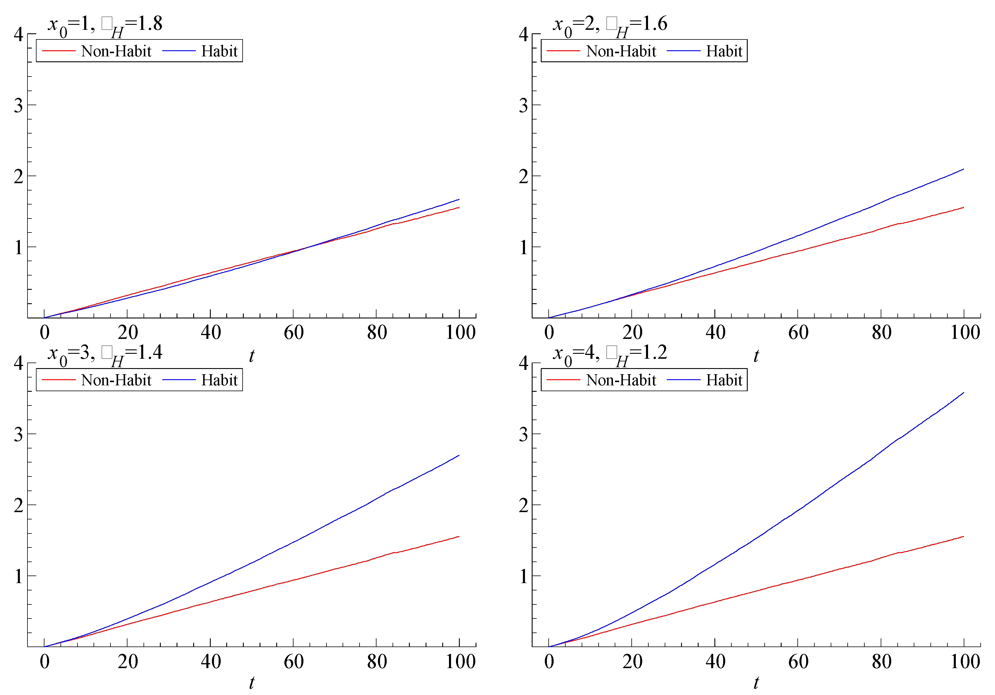
Section 3, reduces the volatility of consumption on the short horizon. Indeed, habit formation has been invoked as a mechanism to help explain the empirical smoothness of consumption. The time series of consumption has lower volatility because the consumption level responds less to changes in wealth, compared to the standard model without habit formation. When the wealth increases, the consumption level increases relatively less and similarly for decreases in wealth. The direct effect of this smoothing is a higher variance for the fund value. Although this effect is partially countered by the more conservative investment portfolio, our numerical investigations indicate that the fund’s value eventually becomes more volatile. This steeper rise in the long-horizon volatility of the fund value may then even be translated into a higher long-horizon volatility of consumption itself. Thus, although the short-horizon variance is lower with habit formation, the long-horizon variance can be higher for consumption as well as for the fund itself. These insights can be gleaned from inspection of the formulae involved. However, numerical simulations presented in
Figure 1 show that the variance of future log-wealth for the case of habit-formation type of smoothing rises much more quickly with the length of the horizon than in the case without such smoothing (in the figure labelled “Non-Habit”).
4 The figure shows four different sets of parameter configurations. For all four configurations, the parameters are set so that the investor with habit preferences has the same initial portfolio composition as the investor without habit formation and a coefficient of relative risk aversion of
.
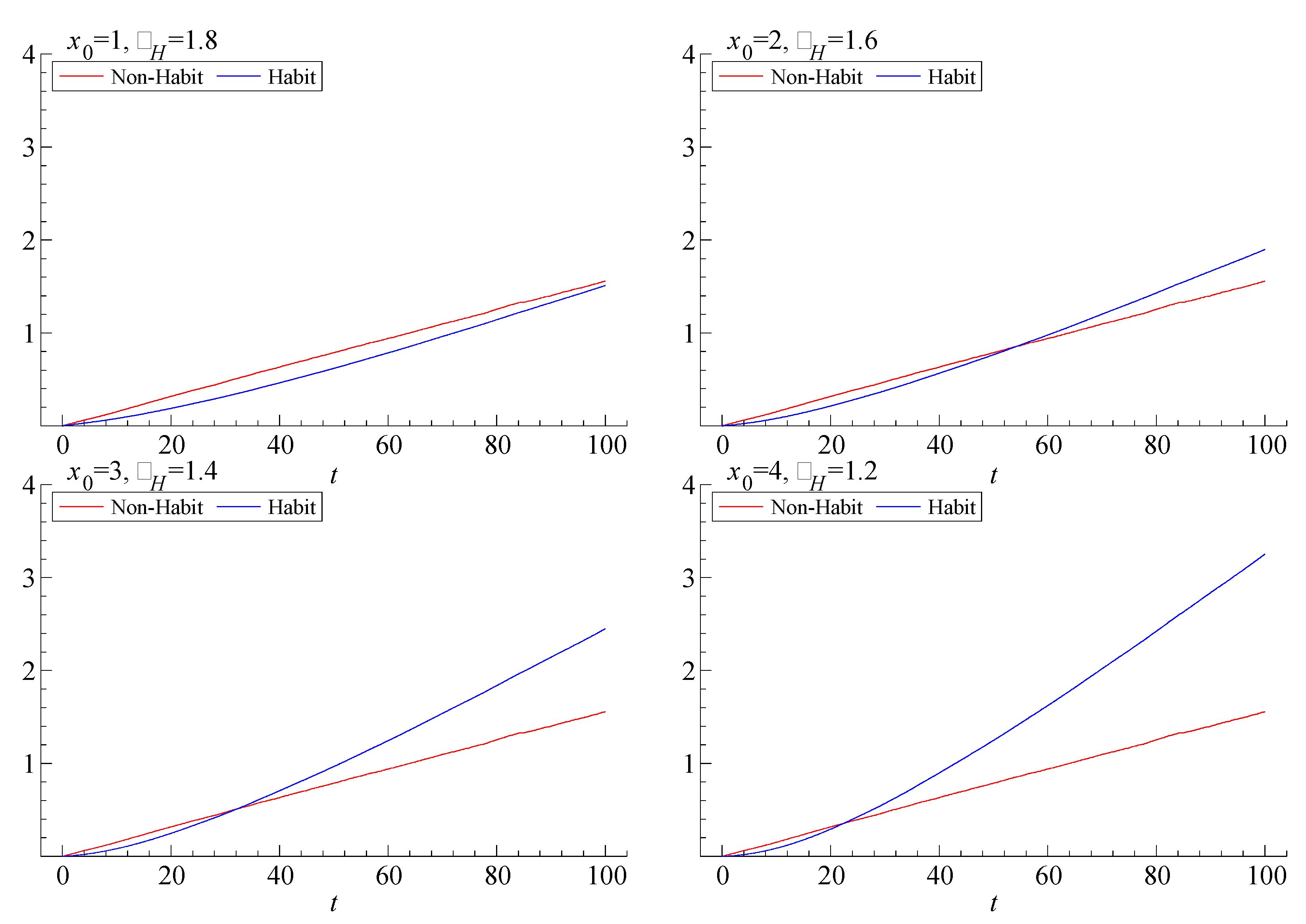
The long-horizon uncertainty of consumption is illustrated in
Figure 2. Here, we plot the variances of log-consumption for different time horizons and for different parameter configurations. In three of the cases, we see lower consumption volatility for “short” horizons (say, less than 20 to 50 years) for the smoothing case than for the base case. However, for longer horizons the smoothing investor can face far more variation in consumption. This increase comes as a consequence of the riskier wealth illustrated in
Figure 1.
This exercise teaches us an important lesson: smoothness comes at a price. We can smooth current consumption by using the fund as a buffer. But then we tamper with the fund’s principal. In so doing, we affect future consumption indirectly and hence future habit levels, which in turn influence consumption even further out. Short-term convenience carries long-term costs.
Provided the smoothing modelled as habits really is part of preferences, the trade-off between short-term smoothness and long-term uncertainty is done optimally.
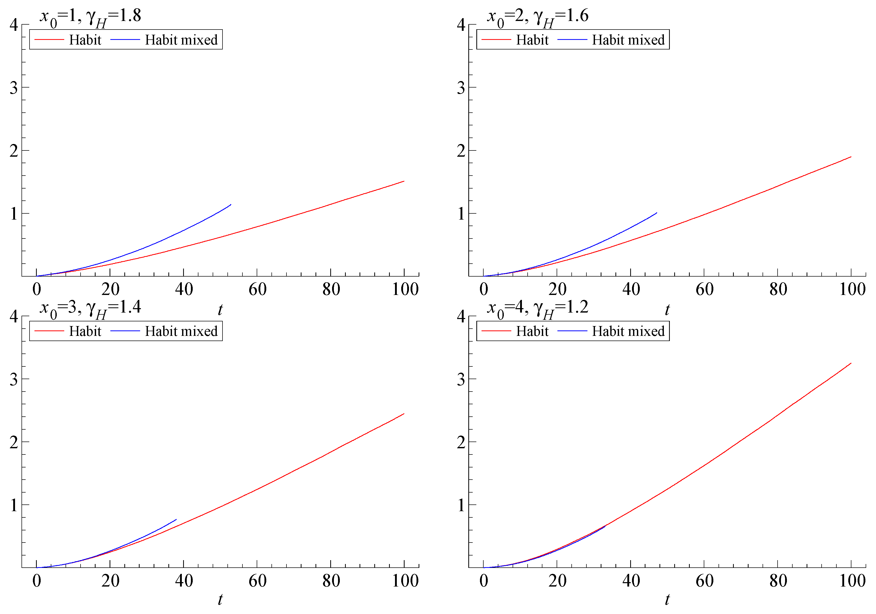
Figure 3 shows what would happen to the variance of log-consumption at various time horizons if the investment and spending decisions were separated so that the risky share of the portfolio were kept constant even though spending is based on the above implications of the habit model. The separation of spending and investment decisions leads to higher variability of consumption. At least as interesting is the fact that the separated rules eventually become inconsistent in all four examples, illustrated by the fact that the graph for the variance of log-consumption ends prematurely for the case of constant equity share (labelled “Habit mixed” in the figure). This phenomenon arises because keeping the risky share fixed fails to safeguard the funding of the minimal, habit-determined rates of future spending for some states of the world. Thus, the investor/consumer ends up in what
Lax (
2002) refers to as the insolvency range.
5We summarize these observations as:
Observation 4. The smoothing of consumption tends to carry a price in the form of a wider uncertainty of the long-run prospects for consumption. This uncertainty is mitigated by the optimal modification of portfolio rebalancing, but it is not removed.
5. Time-Varying Risk-Free Rates
In this section we extend the analysis to account for interest-rate uncertainty. In practice, risk-free rates are not constant over time. In fact, recent decades have seen a long global trend of falling real interest rates since the mid-1980s, as documented, e.g., by
King and Low (
2014) and
Rachel and Smith (
2015). With a less than unit elasticity of intertemporal substitution, a permanent drop in the risk-free rate should obviously imply a corresponding reduction of the optimal draw on an SWF, as indicated by (4b). However, some authors, such as the Organization for Economic Co-operation and Development (
OECD 2014), argue that the recent long decline is likely to be reversed, at least partially. We now turn to the question of what the optimal draw should be under these conditions.
For this purpose, we need a specification of the dynamically stochastic variation in the instantaneous risk-free rate. For tractability, we use the mean-reverting diffusion process introduced by
Vasicek (
1977):
where
is a Wiener process, possibly correlated with
,
is the steady-state riskless return rate,
the speed of return towards this rate after deviations (also known as the force of gravity), and
is the instantaneous standard deviation of
. This specification is consistent with the OECD’s expectation.
When the risk-free rate varies over time, the question also arises whether the equity premium stays constant or whether the expected equity return stays constant instead, so that the equity premium varies inversely with the risk-free rate. We choose to remain agnostic about this issue and use a specification of the equity premium that encompasses both cases:
where
denotes the risk premium if constant (
) and
the expected equity return if that is constant instead (
). With this modification, the diffusion process for wealth now becomes,
In
Appendix A.1 and
Appendix A.4, we carry out the analysis of this case in the absence of habit formation. In
Appendix A.5 we show that an extension to habit formation yields results that are closely approximated by those without habit formation provided that the elasticity of intertemporal substitution is small.
In the absence of habit formation, we note that the Bellman Equation (2) also needs to be modified to allow for the time variation in the riskless rate:
As shown in
Appendix A.1, the time variability of the risk-free rate does not change the result that the optimal draw is proportional to the wealth level. However, the proportionality factor is now a function of the risk-free rate. This function is the solution to a non-linear, second-order differential equation. Although a closed-form solution to this equation may exist, our interest focuses on its semi-elasticity with respect to the risk-free rate. As shown in
Appendix A.4, this elasticity can be approximated around the steady-state risk-free rate of return
by means of the method used by
Campbell and Viceira (
2002) in their Chapter 5.
Appendix A.1,
Appendix A.4 and
Appendix A.5 thus prove the following:
Proposition 3. If the risk-free return varies over time according to (14), the optimal SWF draw, as a ratio of wealth, should respond to time variations in the risk-free rate according to:
provided,
wheredenotes the value ofif the risk-free rate is constant at its steady-state value, as defined in (4b), andis the optimal equity share for.
This result holds as a close approximation even with habit formation provided ε is small.
This intuitive formula shows that the reaction to dynamically stochastic variation in the risk-free rate should have the same sign as the comparative-static response, but be smaller in absolute value because of the expectation of an eventual mean reversion.
6 The difference between the two responses depends positively on
and negatively on
.
means that an increase in the risk-free rate lowers the equity premium and thus reduces the incentive for risk taking, so that the portfolio return is raised by somewhat less than the rise in the riskless rate, which in turn dampens the effect on the optimal draw rate. In contrast,
means that the equity premium is unaffected by the variation in the risk-free rate, so that this dampening disappears.
As expected, the effect on the optimal draw rate is furthermore dampened by , the speed of the mean-reversion adjustment. Thus, the expectation that the risk-free rate eventually returns to normal allows for a smoothing of SWF draws relative to movements in this rate. This is true even if the return path is rocky in the sense of a large . The larger the speed of this mean-reversion adjustment, the stronger the smoothing. If the deviation from the steady state is truly ephemeral (), the smoothing is complete. If, however, the mean reversion is expected to take very long, the smoothing should be very modest.
We summarize this insight as:
Observation 5. The rule for SWF draws should smooth over changes in the risk-free return provided they are temporary. The strength of the optimal smoothing depends on the expected speed of return to normal, even if the return path is rocky. The smoothing should be even stronger if the movements in the risk-free return leaves the expected return on equity unchanged.
Proposition 4. If the risk-free return varies over time according to (14), the optimal equity share becomes:
wheredenotes the theoretical regression coefficient ofon.
Again, the proof is contained in
Appendix A.1 and
Appendix A.4. The first term indicates an inverse relationship between the risk-free rate and the equity share if a drop in the risk-free rate implies a higher equity premium. That would be the case if, as argued by
Hall (
2016) and
Caballero et al. (
2008) regarding the recent long decline in real interest rates, such a decline is due to an increase in the risk aversion of the marginal investor in global markets.
Compared to (4a), this formula furthermore has an additional term which reflects the dynamic risk of future changes in the risk-free rate. We assume
because a drop in the risk-free rate tends to coincide with higher stock valuations, other things being equal. The entire second term, including the minus sign in front of it, is positive provided
, which we view as the normal case. Thus, the risk of a future drop in the risk-free rate calls for a somewhat higher equity share as a dynamic hedge against such a drop. Not surprisingly, this effect is weaker if risk aversion is lower and is actually reversed if risk aversion is very low (
).
7We summarize these insights as
Observation 6. A temporary decline in the risk-free rate calls for an increase in the equity share if this change leaves the expected equity return unchanged. For a reasonably risk-averse investor, the uncertainty of future risk-free rates, furthermore, calls for a somewhat higher equity share as a dynamic hedge provided a drop in the risk-free rate is associated with a higher equity return.
6. Conclusions and Future Work
Using the proceeds of a SWF as a regular supplement to other government revenues makes sense in an advanced economy with a sizeable SWF. However, this practice offers greater complications than it may seem at first.
A rule permitting annual draws corresponding to the expected real return is optimal only under highly restrictive conditions. Our analysis uses Epstein–Zin preferences, which allows us to distinguish between risk aversion and aversion to planned changes over time. Within this framework, we find that a fiscal rule derived from the expected real return is optimal if policy makers’ elasticity of intertemporal substitution is small. However, unless risk is negligible or risk aversion extremely low, the annual draws should be considerably lower than the expected real return as an allowance for risk.
Furthermore, in the presence of risk, such a rule makes fiscal policy bumpy as either tax rates or government services (or both) must move in response to the vagaries of financial markets. This problem can be mitigated by introducing the responses to market returns gradually over time, which we refer to as backward smoothing and the model as habit formation. However, backward smoothing requires lower risk taking, which in turn implies lower return on average. Thus, smoothing can be bought at the expense of lower average SWF draws. Moreover, risk taking must not only be lower, but should move countercyclically relative to the financial markets. Rebalancing should be modified as well so that, in some instances, the SWF should sell rather than buy equity after a stock market decline. Ignoring this implication may lead to premature depletion of the fund. As a final implication, backward smoothing, although dampening short-term uncertainty about SWF draws, will typically increase long-term uncertainty about future draws.
These insights make us critical of the Norwegian fiscal rule. By allowing draws corresponding to the expected real return it ignores risk. By permitting temporary deviations from the real-return rule, it does allow backward smoothing; but it ignores its implications for risk taking and rebalancing.
Our conclusions are somewhat more upbeat in regard to the implications of stochastic movements in the riskless rate over time. When this rate declines, as has been observed in recent years, the SWF draws should decline as well; however, in this case, smoothing does indeed make sense. Moreover, dynamic risks to the instantaneously riskless rate actually call for a somewhat higher equity share as a hedge against the dynamic risk.
We believe these insights to be important food for thought for policy makers in developed countries with sizeable SWFs. However, we also realize that the analysis in this paper only scratches the surface. Just as most households receive labor income in addition to capital income, a government collects taxes. Furthermore, tax revenues as well as spending needs tend to vary with the business cycle, which in turn tends to correlate with stock returns as well as real interest rates. Active, countercyclical fiscal policy adds further volatility to these fluctuations. In the context of an SWF, this means that the policy makers not only want to smooth the draws on the fund relative to returns; they may even want the draws to fluctuate in the opposite direction. Such opposite fluctuations would translate into attacks on the fund’s principal in bad economic times, which could add to the long-term fluctuations and jeopardize the fund’s solvency if caution is not taken.
We intend to take up these and other issues in our future research. As is well known from the context of household behavior, the presence of non-capital income sources presents no new complication if markets are complete. However, this assumption is especially problematic in the context of government finances, as moral hazard, dynamic inconsistency, and poor contract enforceability mean that a government’s future tax revenues cannot be capitalized. As is well known, exact analytical solutions are then no longer available except in uninteresting cases like quadratic utility.
Viceira (
2001) has worked out approximate solutions for optimal consumption and investment for an individual with stochastic labor income under the assumption that permanent changes in labor income are the main determinants of spending behavior.
Benzoni et al. (
2007) similarly study co-integration between stock and labor markets. However, these approaches are unsuitable for studying the implications of cyclical variations in government spending and revenues. Thus, we expect that we will need to rely on simulation exercises to obtain numerical solutions.


