Article

“After End-2008 Structural Changes in Containership Market” and Their Impact on Industry’s Policy

by
Alexandros M. Goulielmos
1,2
1
Department of Maritime Studies, University of Piraeus, 18534 Piraeus, Greece
2
Shipping Division, Business College of Athens, 11528 Athens, Greece
Int. J. Financial Stud. 2018, 6(4), 90; https://doi.org/10.3390/ijfs6040090
Submission received: 20 September 2017 / Revised: 11 April 2018 / Accepted: 20 June 2018 / Published: 1 November 2018
(This article belongs to the Special Issue Alliances, Mergers and Acquisitions in the Shipping Sector)

Abstract

:
The inability of carriers to forecast “demand for containerships” led them to order larger ships. Maritime economists were also unable to forecast it. The new-buildings cut cost per TEU, but “estimated economies of scale” are exhausted with ships beyond 21,000 TEUs, higher than the present. As average cost-AC was not at minimum, carriers did not produce at minimum efficient scale (MES). As larger ships are more competitive, smaller ships led to laid-up, and eventually scrapped. This strategy, however, did not bring the desirable balance between demand and supply. Due to falling demand, following the meltdown at the end of 2008, carriers priced their services at marginal cost-MC, and thus they accumulated losses. As a result, carriers resorted to frequent GRIs (freight rate increases). Supply exceeded demand and average distances fell after 2008. Containership market will remain depressed if economies of scale lead carriers to shipyards. Scrapping—the last hope—removed only 1/7 of the oversupply. Revenue, operating profits, and net profits, due to increased financial expenses, were lower than in the past. Aggressive ship-building programs could not be carried-out, because the depression meant that there are available only limited funds. The estimated funds required for new buildings were as high as $4 billion per carrier. So, the sector is in a vicious circle. The only helpful sign was the reduction in fuel prices after 2011 from $800/ton to $278 (2015). We also showed that ports and canals, through their traditional charging policy on size, penalized containerships for their efficiency—if volume discounts are not provided. Port dues and container handling and canal dues account for as much as 40% of the annualized containership cost. Finally, to study the relationship between concentration (market share) and revenue, operating profit and net profit, we ran three regressions; but only one gave a high correlation coefficient (0.97). This suggests that the containership market is purely competitive. We also showed that the Herfindahl index was 683 units (i.e., <1000) and Lerner’s index was 0.55—both indicating oligopolistic trends. Our model shows that containership market is either oligopolistic or purely competitive. This finding shows the double face of containership markets, which so much confused maritime economists.

1. Introduction

This paper combined theory with empirical evidence from the containership market-CM. The theory applied was that of “maritime industrial economics”1. After end- 2008, conditions in CM (freight markets) changed from prosperity to depression.
In the past, CM attracted the consistent research attention of maritime economists. However, they reached no consensus over its market structure2. The papers we studied, of which 12 are reviewed in next section, argued that CM is: contestable, a two-stage duopoly, a perfect competitive model, a SCP case-study, a Porter’s model, a dual oligopoly, a monopolistic competition and, above all, a game3 (2002–2017).
The CM was depressed before 2000 and after 2008. New building prices fell, along with time charters, and second-hand ship prices. From 2000 to 2005 CM gradually recovered, and chartering conditions improved. From 2005 to 2008, the 2nd hand market was more active. From 2006 to 2010, containerized trade fell, and recovered between 2011 and 2017, but its growth rates were lower than those before the end of 2008.
The CM showed apparent “empty economies of scale” (eES), meaning that there was no demand for big ships. eES are manifested in larger containerships, introduced into the world fleet in large quantities in 2006, i.e., 15,550 TEUs (up 69%, compared with 9200 TEUs in 2005), and 18,270 TEUs in 2013 (up 17.5%). Ships in building in 2017 were of a size over 21,000 TEUs…
The meltdown at the end of 2008 caused container freight rates to decline in a steady way, and to reach record low levels. This was due to a combination of a weakening demand and the entry of ever larger container vessels, even after the end of 2008. Moreover, container freight rates became volatile after 2009 over their 3 main trade routes. Although shipped cargo rose by approximately 6%, revenue reduced by 3%, between 2013 and 2014, indicating an inability to sustain freight rates in the face of increased supply, coupled with falling distances.
In addition, a main concern that affected all ships was the climatic change, especially after the Paris conference and Trump administration (http://time.com/5058736/climate-change-macron-trump-paris-conference/ downloaded 08/10/2018). So, the focus is also on environmentally-friendly technologies, meaning ships with reduced gas emissions.
One positive development occurred: the total fuel consumption of containerships reduced, contributing to better climate, through lower CO2 emissions, as a result of slow steaming (SS). SS improves environment and decreases carriers’ expenses (on fuel). One negative development also occurred because SS produced longer4 transit times (inferior service quality of CM).

2. Aim of the Paper

The main theoretical aim of the paper is to propose a model for CM, and to clear, if it is at all possible, the confusion about its structure. Another objective is to show that the industry is in disequilibrium, as MC is < AC (for ships of 15,000 TEUs). Moreover, we wish to show that, if carriers are rational, they should apply economies of scale, aiming at forcing rivals to scrap their inefficient tonnage. We aim also to show that the imbalance of supply and demand, and the shorter distances witnessed, were the causes of current depression, which lasted beyond end of 2008. Finally, we aim to examine an issue of great importance for policy, namely: the relationship between concentration (market share), revenue, operating profits, and net profits. Moreover, we drew attention as to whether high canal, port and container handling expenses (currently at 40.5% of carriers’ costs) distort industry’s propensity to economize by building larger ships (economies of scale).

3. Structure of Paper

The next section provides a literature review, followed by a “description of the current market”; this is a picture of the forest before examining its individual trees. Then, we analyzed “the primary causes of depression” followed by the issue of “economies of scale”. Next is the “investigation of the market structure of the CM industry”. A short account of carriers’ expenses follows. Finally, the paper’s model is presented, followed by conclusions.

4. Literature Review

Song and Panayides (2002) adopted a game theoretical approach based on the 1953 “Von Neumann and Morgenstern” theory, assuming that utility is measured. Cullinane and Lee (2002) criticized them, because “qualitative influences on liner companies are adequate to make carriers cooperate”. Notteboom (2002) used a contestability model, but he found out that CM puts certain barriers to entry.
Lam et al. (2007)—using SCP5—argued that the cross-sectional analysis6 they applied, provided no conclusive evidence that increased concentration (of slot capacity), or attempts by shipping lines to boost potential slot capacity—mainly through collaborative agreements—improved financial performance7. Markets remained contestable.
Sys (2009) applied 4 concentration ratios to data from 1999 to 2009, and concluded that CM operates in a double oligopolistic market structure (Table 1). Ducruet et al. (2010) argued that port and maritime studies on containerization showed a global traffic concentration8, where a liner services network aims at a best trade-off between cutting operational costs (using economies of scale) and reducing calls; this led to an even higher concentration9.
Strandenes (2012) questioned whether CM remained contestable. She instead argued that the reduction of freight rates (per TEU), the fall in charter rates, and financial crises, as well the reduction in economic activity (2009), suggested that the industry was unable to withstand the pressure on freight and time charter rates through cooperation.
Maloni et al. (2013) investigated the SS practice of container carriers (end 2008–2012). SS led to fuel efficiency and lower GHG emissions. A speed of 18 knots, instead of 24, reduced total cost by approximately 20%. Also, 43% lesser carbon dioxide’s emissions. In $ terms, SS provided roughly $585 m a year in savings (in 2010: $700/MT fuel price; and in 2013: $600). Shippers, however, paid $951 m for pipeline inventory costs. This alternatively is the cost of reducing the quality of service10.
Bae et al. (2013) presented a two-stage duopoly model of container port competition (transshipment). They showed that shipping lines assign more calls to ports by providing lower prices and larger capacity. Carriers preferred ports providing higher transshipment levels if were free of congestion.
Ferrari et al. (2015) examined the impact of SS on fuel costs (after April 2008). SS reduced excess supply, saved fuel cost, which had a 43.5% average share in total operating costs (for 4000–10,000 TEUs), and reduced emissions. At the same time, however, freight rates fell11.
Niamié and Germain (2014) found six strategies all in all looking at 41 studies: one was differentiation, from 1997 to 2005, which occupied 10% of all studies. This was followed by alliances, 1997–2013, by 34.5%; cost leadership by 12%, 1997–2011; diversification 17% from 1997 to 2013; specialization 19.5%, from 2002 to 2011 and concentration 7%, from 2005 to 2008. So, diversification and alliances (more than 50% of the studies) are the strategies that were widely applied before 2013.
Kou and Luo (2016) studied overcapacity in the CM in a duopoly game. They concluded that capacity expansion is rational12 during troughs, leading to chronic oversupply and persistent low freight rates. In the capacity expansion game, the Nash equilibrium dictates: “expand”, “expand” for both firms. Firms do not necessarily achieve maximization of profits. The expansion of one firm causes freight rates to fall for both. They argued that persistent overcapacity leads to an early retirement of -old or inefficient- vessels, something confirmed by this paper.
Lin et al. (2017) argued that carriers build collaborative relationships with other carriers, competing with each other, to optimize profits. They used a coopetition game13 to determine optimal level.

5. Data Used and Methodology Adopted

The sources of data are several. But the main ones are those of UNCTAD (2016) and of Drewry Shipping Consultants Ltd. (2010). Moreover, numbers found in the papers of Furuichi and Otsuka (2015), Lam et al. (2007), and Sys et al. (2011), were used to run-out 3 regressions and construct a number of figures.
As far as methodology is concerned, it is our method to prove our arguments by creating figures, simple regression and/or mathematical models as the case may be. The model, which was applied for the first time, is presented as Figure 13, showing the double face of the CM.
This paper places more stress on the empirical verification of the postulates and paid a great deal of attention to the facts of experience—known as “historical method”.

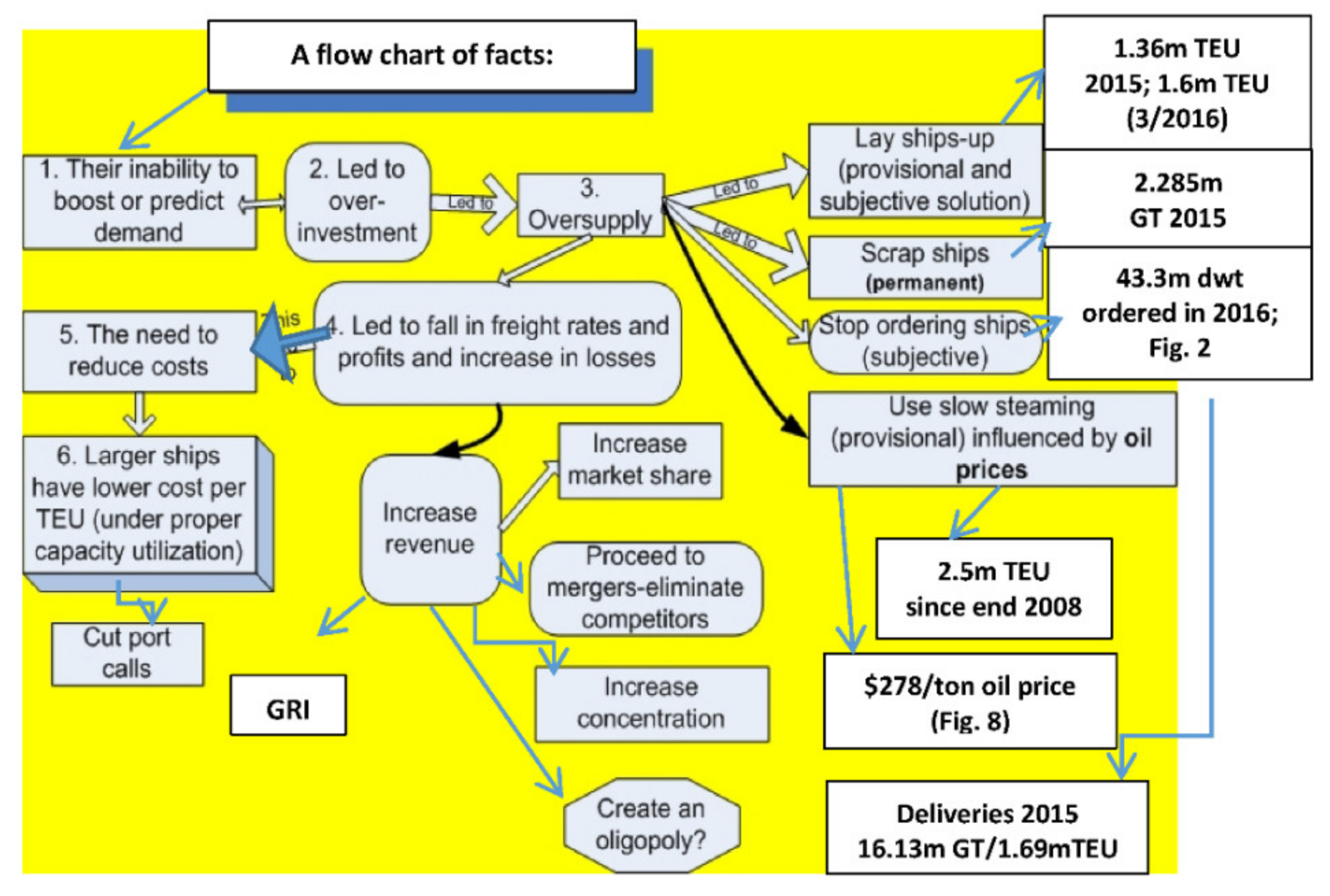
6. An Overall Picture of the CM

• The main picture
CM is like a dense forest and thus we decided to present it next (Figure 1) before examining its individual trees.
It seems that carriers cannot forecast demand, so they adopt the idea that demand will rise (UNCTAD 2016). Moreover, maritime economists also were unable to forecast demand for containerships (Munim and Schramm 2016). (As a result, they order (larger) containerships, which indeed provide lower (theoretically) AC. Carriers do not know that economies of scale (ES) are not exhausted now (at 15,000 TEUs) (as shown in Figure 6b), and thus industry does not tend toward equilibrium, where MC = AC. The reduced trade, due to the meltdown at the end of 2008, and the larger ships built, created oversupply—with falling freight rates, GRIs, SS, lay-ups, cut of frequent port calls, scrapping and co-operations—as well “competition among the few”.
There was an interesting pattern of the containership orders (Figure 2). Purchasing was not uniform, but mixed among liner companies, supporting our argument that “new-buildings may harm net profits”. This explains why certain industry leaders14 (A.P. Moller-Maersk) resisted proceeding to new-buildings.
In 2013, the orders were 1.7m TEUs costing $19.2b (~$11,294/per TEU), which gives ~24,000 TEUs per dwt (Kou and Luo 2016). The 18 major carriers earned $126.4b in 2008; so, the cost of the above orders needed 15.2% of total revenue (Sys et al. 2011). In 2002, the turnover of the 16 out of 18 major carriers was ~$55b, the operating profit was ~$3.5b, and the net profit was $278m (Lam et al. 2007). So, the net profits of 2002 could not finance orders placed, without a substantial external financing of an estimated extra amount of ~$2b for the 18 carriers for which we found data.
“Liner firms” are the one player in the CM and “charter-vessel owners” are the other. The latter are the independents (e.g., Danaos; Seaspan15). The latter arrange financing and chartering of the largest ships for the first 8–12 years of their life. Independents16, we believe, are more efficient, and freight rates are negotiated between these two players. Independents also have a greater share in the building of the new larger ships (75% in 2007).
The new orders on 10 March 2008, of the 20 top companies were 4.93m TEUs, or ~50% of their 9.92m TEUs existing fleet. Among the top 20 companies, the percentage of new orders varied from 17.4% (Evergreen) to 99.7% (Zim) (Lorange 2009) of carrier’s existing fleet, as mentioned above. COSCO had new ships on order (and ships chartered-in) in 2008, amounting to 117% of its existing fleet. Five companies had roughly 50%, and the rest had less. This indicates the different newbuilding strategies among the carriers. This raises the question of who had the right strategy.

6.1. Scrapping

Scrapping -approximately 10% of the world total tonnage of containerships- was the hope to cancel, or even exceed, deliveries, and cope with the depression. Scrapping of containerships was, in 2015, roughly 2.3m GT, or only 14.3% of deliveries (16.1m GT) (Figure 1).

6.2. Lay-Up and SS

Lay-up and SS camouflage the problem of oversupply, because in these two cases, ships go and then can come back. There is a basic difference, however. In lay-up, carriers pay, while in SS carriers economize. SS is estimated to have absorbed 2.5m TEUs since the end of 2008. Lay-up tonnage was 1.36m TEUs (2015) or only 7% of the existing fleet. Since the main year of depression, 2009, lay-up was 1.5m TEUs or ~12% of fleet capacity, and in 2016 it was 1.4m TEUs (Figure 1).

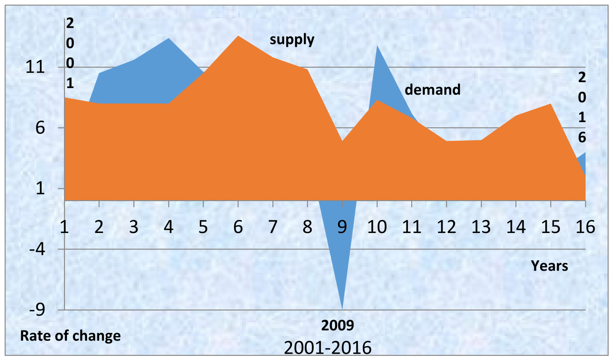
7. Imbalance of Demand and Supply

In shipping, as in all industries, demand and supply analysis is basic17. Demand in CM grew roughly 13% in 2010, but in 2009 fell 9%. Between 2011 and 2014 it rose 5%; in 2015, 2.3% and in 2016, 4.2%.

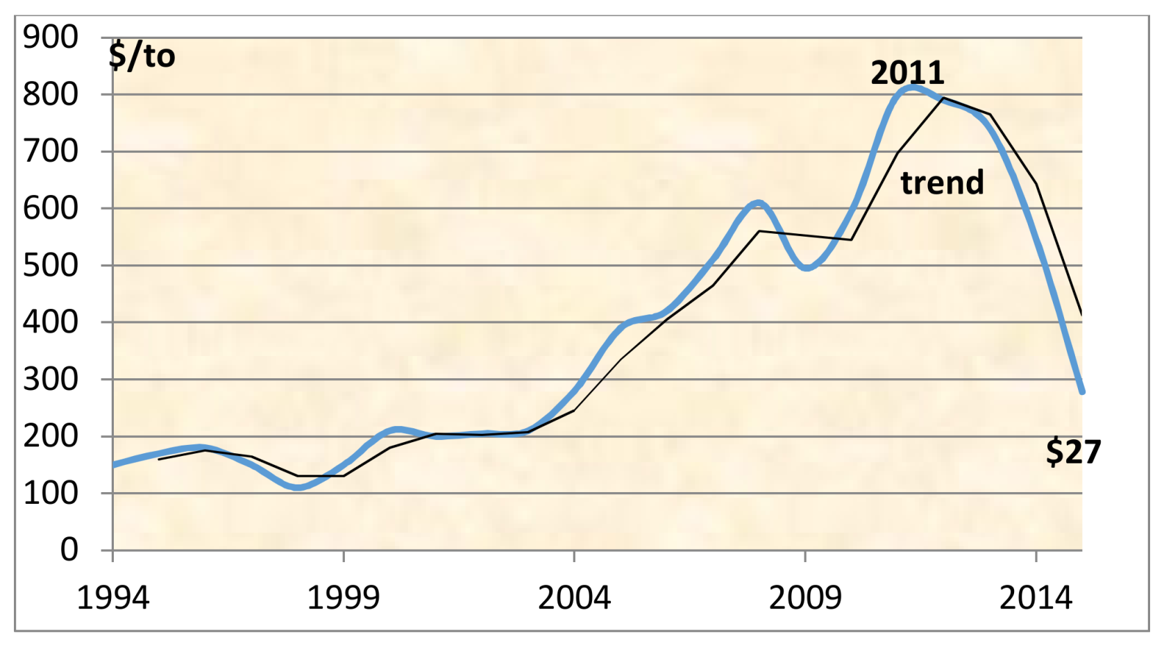
7.1. Value of Containerized Trade

The value of containerized trade is estimated at €6.84 trillion (171m TEUs*€40,000) in 2014 (Wang et al. 2017). The “major”18 liner companies obtained $173b (2015). This means that the 2014 revenue was 1/4 of that in the past19 (assuming 1$ = 1€).

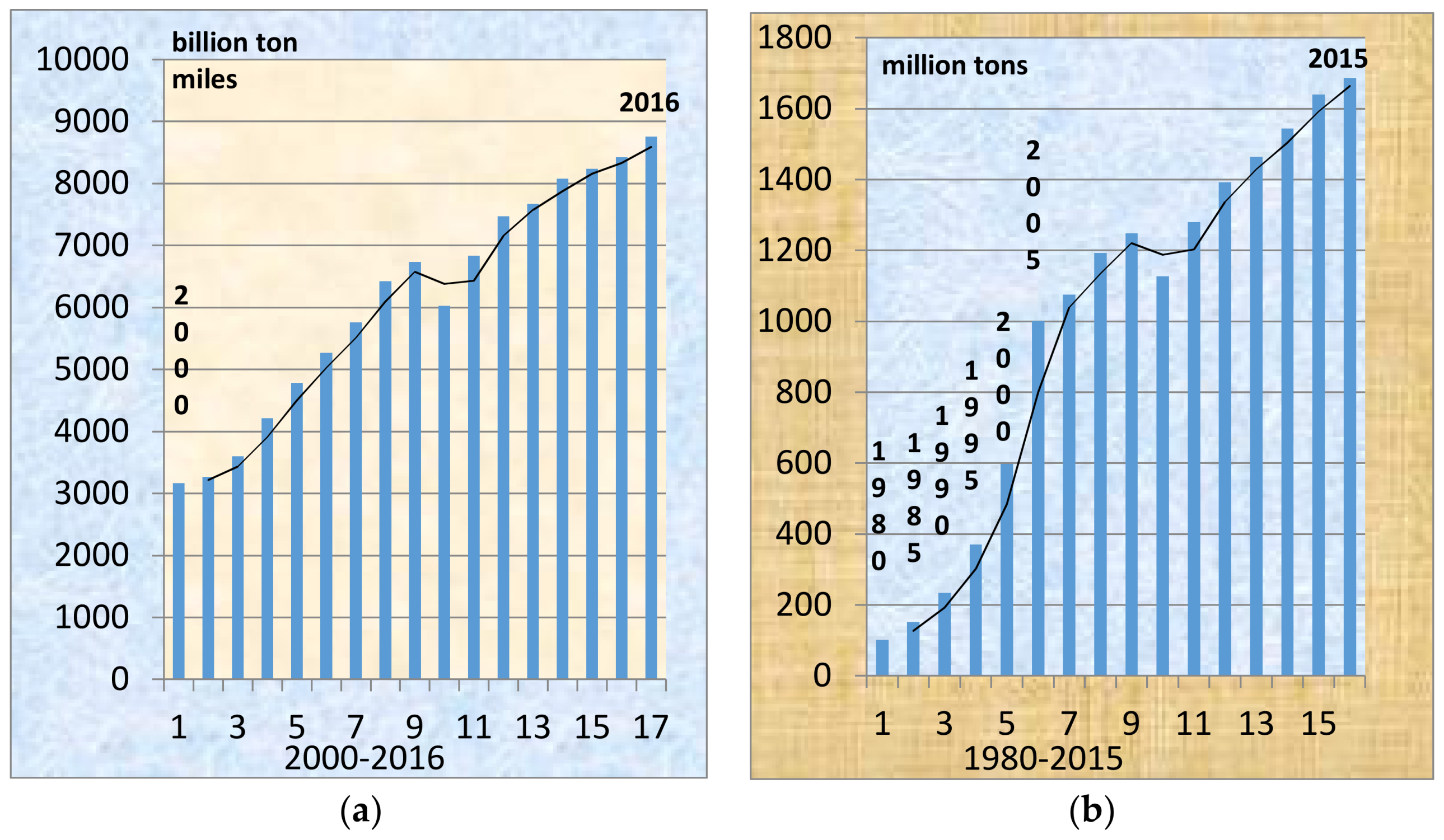
7.2. Volume of Containerized Trade
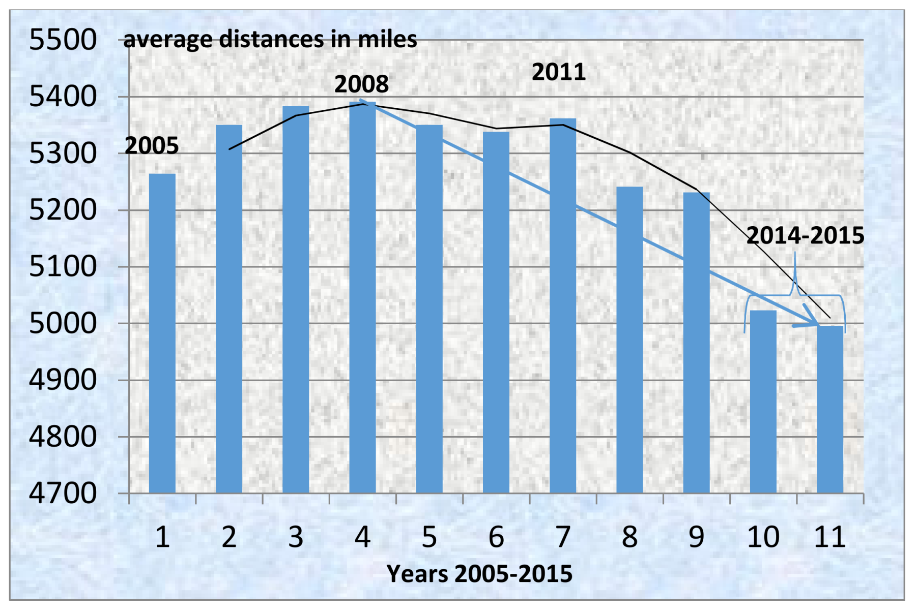
The containerized trade achieved exceptional statistics, increasing 16.5 times since 1980, from 102mt to 1687mt in 2015. It recovered in 2010 (Figure 3a). Moreover, the total shipboard capacity employed grew in 2014 by 8%—but only by 1% in 2015–2016—from 18.25m TEU in 2014 to 19.73m in 2015 and 19.85m in end-July 2016 (UNCTAD 2016).
Demand, of 175m TEUs (2011), 171m TEUs (2014), and 180m TEUs (2015) (up 2.86% between 2011 and 2015), was unable to cover existing supply, of 240.3m dwt (July 2016). The sector had reduced revenue between 2011 and 2015, from $204b to $173b (down 15.2%) due to a weaker demand and lower freight rates (UNCTAD 2016).
Figure 3 presents the containerized seaborne trade between 2000 and 2016 in million tons, and between 1980 and 2015—for selected years—in billion ton-miles to show the effect of distances.
In 2009, seaborne trade fell in both ton miles and tons. Demand did not assume, after 2009, the growth rates it had before (trend lines). In fact, it is estimated that demand reduced by 4000 billion ton miles between 2010 and 2016 and 1700 million tons up to 2015 (b)—by projecting trends linearly to 2015 or to 2016. In fact, between 2006 and 2010, trade rose by 250 million tons instead of 400 million tons as it had between 2000 and 2005 and as it did between 2011 and 2015 (a drop of 37.5%).

7.3. Distances

Demand was also weaker due to shorter distances (Figure 4). This means that containers were transported over shorter distances.
Average distances fell after 2011, and especially during 2014 and 2015: from a high 5391 miles in 2008 to 4996 in 2015 (fall about 8%).

7.4. Balance of Supply and Demand

Demand (TEU million lifts) grew faster than supply (which is taken as the total capacity of the containership fleet) from 2002 to 2004, and marginally in 2005 (+0.1%) (Figure 5). It fell from 2006 to 2009. In 2010–11, it grew faster, but slowed down between 2012 and 2015. In 2013 supply and demand grew equally (5%). In 2016, the growth was 2% for demand (projected).
The balance between the growth rates of demand and supply have long been suggested by Koopmans (1939, for the tanker market) as a determinant of freight rate equilibrium, but he was neglected.

8. Strategy of Economies of Scale during a Depression

8.1. Apparent Paradox

Containerships were never bigger, and container freight rates were never lower (UNCTAD 2016). In a depression, the laid-up tonnage is a strong indicator of market conditions, and also indicates the psychology of owners, the depth of depression, and also the illusion that there will be a rapid solution. In March 2016, the laid-up tonnage for containerships stood at 1.6m TEUs (http://www.alphaliner.com) or ~0.89% of the 180m TEUs demand.

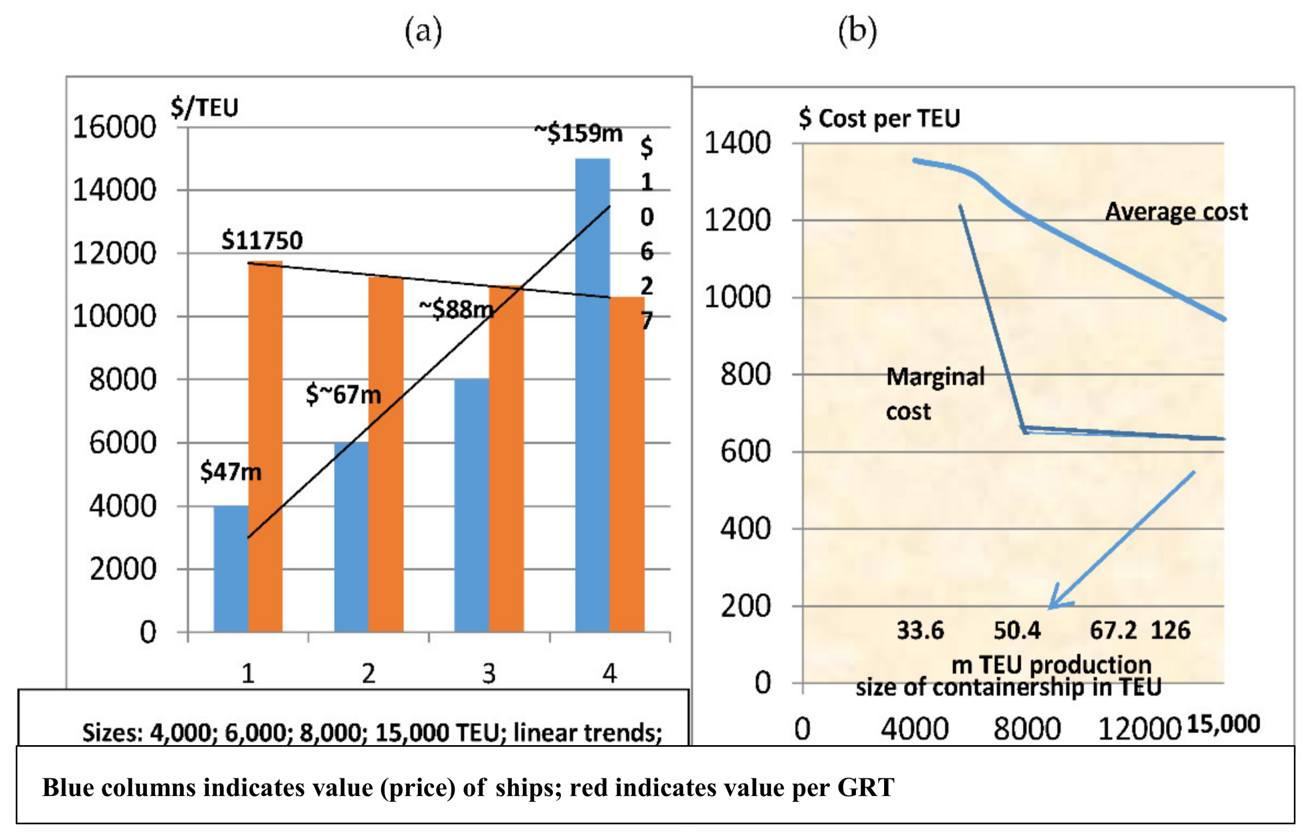
8.2. Economies of Scale (ES)

ES exists when AC (cost per TEU in the long run) declines, and production (in TEUs) increases. This, however, is a double edged sword: larger ships with lesser trade mean fewer ships needed for the same job… Surplus containerships are laid-up because of lack of business—usually after a delay, during which the owner hopes for the market to turn up20. Ships in lay-up are those of higher daily operating costs than prevailing freight rate, not necessarily used/older ones.
As shown in Figure 6b, AC fell as the size of containerships increased from 4000 TEU to 15,000 TEU: i.e., from $1355/TEU to $944 (over 12 voyages per year via Suez Canal). MC21 also fell from 6000 TEUs to 15,000 TEUs: from $1249/TEU to $645.5022. Average costs fell faster, especially from 8000 TEUs to 15,000 TEUs (down 22%). In this case, total cost rose by 47%, but production almost doubled (1.875 times). Apparently, economies of scale exist also beyond 21,000 TEUs, or even 40,000 TEUs, as AC is not at its minimum at 15,000TEUs (the so called minimum efficient size or scale-MES).
Average revenue-AR (for ‘major’ companies), derived from total revenue of $204b in 2011 resulting from 175m TEUs carried (AR2011 = $1166). The revenue in 2015 was $173b from 180m TEUs carried23 (AR2015 = $961). If we define MR as the change in total revenue from the sale of an additional TEU, then MR2015 is down to $620 ($31b down in total over 5m TEU for the period 2011 to 2015). This means that if major companies want to carry (5m) additional TEUs, they had to accept a lower price (on all TEUs). This is one sign of market imperfection. In Figure 7, the curve MR indicates that by expanding production beyond OQ, MR is negative, as shown above, at −$620.
If MR is negative -as above- then why would a firm choose to expand? One justification for the firm/carrier to expand beyond OQ is if it obliges a rival to scrap an equivalent tonnage24. Profits are also increased (Train 1991). A negative MR implies inelastic demand, because if ed < 1, then MR < 0. The firm faces elastic demand by producing OQfirm ≤ OQ. As shown, elasticity of demand is equal to 1 in the middle of the demand curve and ed > 1 on the left part and ed < 1 on the right part of the demand curve.
Figure 6b indicates no diseconomies of scale (AC > MC). The composition25 of total (annual) unit costs taken into account here was: 43.4% for fuel, 28.5% for port dues and container handling, 13.3% for annual capital cost26 and ~12% for canal dues (giving a total of 97.2%). Management apparently tries to reduce all above costs, if it can, during a depression. First fuel costs are reduced by SS, and then port dues etc., by offering fewer calls/passages. Capital cost can be reduced by using best timing when placing an order for a new building. Fuel costs, however, depend primarily on fuel prices27 (Figure 12), and cannot be influenced by carriers, except by SS.

8.3. Costs Due to Size

Studying ES, there are also costs related to size, like port and canal dues, and costs related to a ship’s NRT (or GRT/GT) and the costs of empty containers. So, the larger the ship, the more she has to avoid frequent uses of ports and canals, at least during a low market.
Ports should treat big containerships sympathetically, we believe28. In a depression, carriers had to increase TEUs per shipment by cutting down frequent visits, and increasing ships’ capacity utilization29. In a depression, carriers30 tend to select the most profitable routes (Lorange 2009, pp. 205–11).
ES are theoretical, if they do not follow economies of density. In the airline industry, economics of density are ES along a route. To reduce AC, the route traffic volume has to be increased. In CM, the route traffic volume is found from the revenue from TEU miles (RTM). This is the number of TEUs in a particular route, multiplied by the miles that these TEUs were carried. This is what has to be maximized.
In Figure 6a, capital costs per year fell per TEU from $11,750 to $10,627 (a drop of $1123/TEU, or $12.3m revenue on the extra 11,000 TEUs, increased from 4000 TEUs to 15,000TEUs). ES are tempting for carriers at all times, but they are only available if there are additional shippers to pay the extra $12.3m, as shown above. The cost to build a containership rose from $47m (4000 TEUs) to $159.4m (15,000 TEUs). Thus, the size rose 3.75 times, while building cost rose only 3.39 times. Depressions also create lower building prices, but the extra 11,000 TEUs is important as it can bring in about $7m (taking the Shanghai–Northern Europe route as example) per charter (or $84m per year). ES were obtained by Mediterranean Shipping Co and China Shipping Container Lines, which employed a ship of 19,000 TEUs (2012) (Wang et al. 2017) and of 21,000 TEUs (Gharehgozli et al. 2017).
Figure 8 shows that total cost is not proportional to production, as it does not follow the 45° line. Especially after a total annual production of 40,000 TEUs, total costs fall sharply. So, carriers are right to pursue higher production on the basis of a theoretical lower cost per TEU.

9. Market Structure of CM

9.1. Is CM Contestable?

This is a situation where the market insiders avoid contesting with, or provoking the, outsiders, for the fear that the latter will enter into the market. One strong provoking element for entry is a high rice, leading to super-normal profits. Fear, according to theory, prevents insiders from setting high prices (meaning prices above perfect competition): (Baumol et al. 1982).
When contestable theory applied to airline industry, this was not a perfect contestability31 case. Maritime exit costs -by the way- can be substantial, despite the existence of a well-organized 2nd hand ship market (e.g., Hanjin’s exit from the sector by bankruptcy, mentioned below). In contestable markets32 entry or exit costs can be positive (sunk costs > 0). One step towards more contestability in CM, was the change in EU’s policies in 200833.
Given the building price of a single containership of 15,000 TEUs in 2013 of approximately $159m, the market cannot be perfectly contestable. Sunk costs are not zero as an exit, which is more likely during a depression, lowers 2nd hand ship prices.
Hanjin (est. 1977) exited the CM due to falling freight rates, the slump at the end of 2008 and the excess supply. On 17 February 2017, the company declared bankruptcy. What is the cost of its exit? We estimate that it was high. The company’s ships were stuck in ports and canals waiting for cash. The company’s assets were confiscated. Some assets—ships—were sold at auctions. The company’s 14 dockyards were sold. In addition, the timing of the exit was wrong. We do not believe that Hanjin will ever reach the estimated liquidation amount of $153bn.

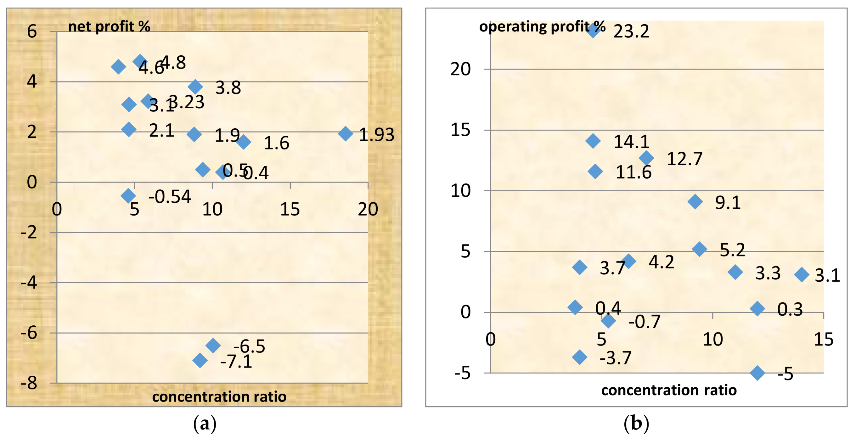
9.2. Can “Concentration” Help Containership Companies’ Profits?

CMs are characterized by increasing concentration over time, mainly in capacity. Concentration is a reasonably accurate predictor of the likely nature of competition. It is measured by a number of formulas about market structure: i.e., measures using the number and the distribution of firms within an industry. The concentration ratios in CM vary from year to year, from market route to market route34, and also from direction of transport to direction (e.g., eastbound/westbound) and from port to port.
The container-carrying capacity per provider per country rose 3 times in the last 11 years, but the average number of companies providing services from/to each country’s ports, decreased by roughly 1/3 (29%). The number of liner shipping companies on average per country fell from 22.1 in 2004 to 14.6 in 2016 (UNCTAD 2016).
• CRn Concentration Ratio
A common concentration ratio is CRn for the shares of the n top companies. Especially35 if n = 4 . CR4 equals to i = 1 4 S i [1], where S is the share of one company compared to the other 3. At the end of July 2016,36 CR4 was 46%—down from 47% in 2014. For the top 20 companies, CR20 was 87% in 2016 down from 89.5% in 2014, close to the scheduled passenger air transportation levels, which had 50% for CR4 and 90% for CR10 respectively in 200737,38. A CR4 = 65% attracts antitrust interest (in Canada). Moreover, collusion is expected in industries with CR4 > 40%39.
• CM Concentration and Profitability
Did increased concentration40 (of slot capacity etc.) in liner shipping result in better financial performance? In Figure 9, the regression between net profit—as a percentage of turnover—and CR4, and CR10, for Transpacific, Europe–Far East, and Transatlantic routes (in 2002), is shown.
As shown, (in Part a) the net profit of 14 carriers derived from their turnover after deducting costs of services/operating expenses41 increased (in 2 distinct and rather close vertical blocks), as concentration rose42,43. The higher net profits were reached by NYK = 4.8%; MOL 4.6%; HPL (Hapag-Lloyd) 3.8% and HYU (Hyundai) 3.1%, with concentration ratios of NYK 5.3%; MOL 4%; HPL 9%; and HYU 4.6%. The correlation coefficient44 between net profit and concentration, however, is negative, and equal to 0.51.
Figure 9b shows the operating profit before finance and taxation, which accountants argue is a superior measure of performance (Reid and Myddelton 2005). The pattern of profitability and concentration did not change for the 15 carriers this time, showing that the five most efficient carriers are NYK, MOL, MSK (Maersk), HPL, and KLN.
NYK stands-out, as its operating profit fell from 23.2% ($577m) to only 4.78% ($119m) in 2002. We believe carriers reduced their net profit, if they had heavy finance costs (and taxes). Financing from net profits is difficult in extensive shipbuilding programs, as a 15,000 TEUs vessel cost $159m in 2013. However, this correlation coefficient is also negative, and equal to 0.27.
Regressions had to run over the same45 market: e.g., one market/route is Transpacific eastbound and another is Transpacific westbound. This indicates how important is to define first the market46. One can speak also of monopolistic competition47, if one demonstrates that geography produces non-homogeneous services. Excess capacity in CM is beyond doubt. The difficulty is that the homogeneity of services is a property that depends on psychology.
The above situation is the same as that of the 9 major US airlines in 2010 (Besanko et al. 2013). Delta had a 21% market share (first), but only a 9% profit margin (net profit as a % of revenue), and a unit cost 5% higher than the industry’s average. Alaska was the most profitable with a 14% profit margin and 14% lower unit cost, but a very low (2.6%) market share. JetBlue was the most efficient with 29% lower unit cost and 9% profit margin, but a rather low (3.6%) market share. So, higher market shares in airlines, do not create higher profit margins, while lower costs do. This is a point where all economists agree.
There is a high correlation coefficient (0.97 < 1.00) found between the market shares (in %) of 18 liner operators (out of top 100), in 2010, and total revenue (US $m in 2008) (Figure 10). This is not as obvious as it may look, as a liner can attract many TEUs to transport at a rather low freight rate per TEU. These carriers owned 8.01m TEUs (01/01/2010), had a 65% market share, and $126.4b revenue. The regressed variables belong to two different years. The top 4 had a CR4 of 51% in TEUs and 50% in revenue.
As Martin (2010) argued in another context, concentration is a consequence of factors limiting the number of existing firms in equilibrium, and/or giving to first movers certain advantages.
• Oligopoly in CM?
Sys (2009) reached the following conclusions (Table 1) in her doctoral thesis. Later (Sys et al. 2011) she argued48 that CM is a “monopolistic competition”.

9.3. The Herfindahl Index51
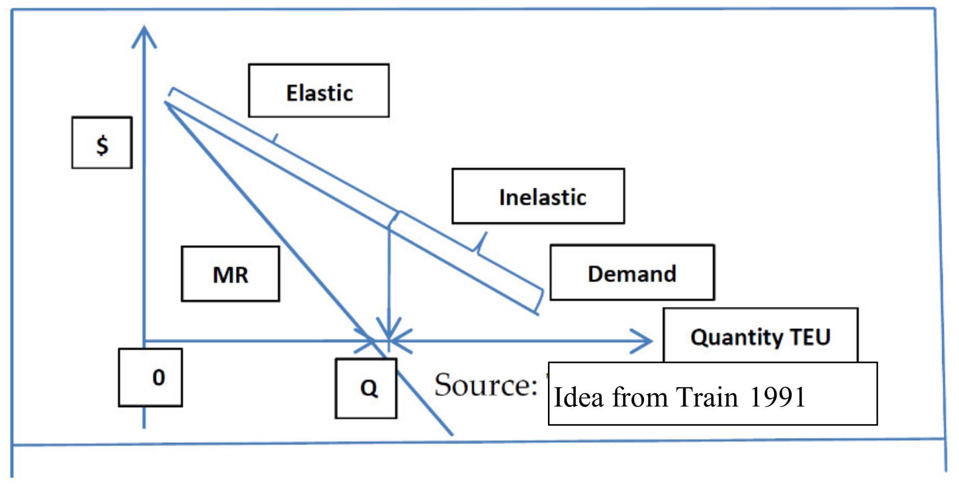
A superior measure of market structure is the Herfindahl index52: H = i = 1 n ( S i ) 2 [2], where S is the share of each firm in a total for n firms. H is a statistical measure of the extent of concentration of the market shares in an industry. Based on the market shares (%) of the leading 50 liner shipping companies by total shipboard capacity deployed in TEUs53, and for n = 36 (end-July) (excluding shares of 0.01, which do not affect the index when squared) (Besanko et al. 2013; Sys 2009), H54 is equal to 683. This value is below the moderate concentration benchmark of 1000. In USA transactions that increase HHI by more than 100 points, in a concentrated market with H ≥ 1801, anti-trust concerns are triggered (US Department of Justice 2006).
Goulielmos (2017) showed that HHI2008–2010 varied from 766 to 1777.555 on revenue, depending on the number of carriers. He also found oligopoly HHI 2002 = 0.31 in the turnover of the four top carriers56. Over trade routes, he found HHI 1998 2002 = 645 , which is < than the 1000 units.

9.4. Lerner’s Index

Lerner’s index—LI (Appendix A)—measures monopoly (and oligopoly) power. LI = (price less MC)/price or P-MC/P [3]. Perfect competition (and perfect contestability) requires P = MC = MR and LI = 0 . Oligopoly requires 0 < LI 0.80 . Monopoly requires 0.81 < LI 1 . The higher LI, the more concentration there is, and the more power firms have to exceed normal profits.
In the “Shanghai to West Africa (Lagos)” route the freight rate was, in 2015, $1449/TEU, so LI = 0.55. This57 means that CM is neither a perfect competition nor a contestable market. Exceptions are the 5 out of 18 Intra-Asian freight markets58. So, LI indicates that increased oligopoly power is found over certain routes, and but not in others59. This supports our model presented in Figure 13.
• Market Equilibrium
Given that supply and demand determine price (Figure 11), the monopoly price is OP, where MR = MC , and production is OQ (in TEUs). The monopoly power is ( O P M C ) / OP ( = LI ) . CM is not in equilibrium60, however, as AC > MC for all current production, due to unexploited ES at 15,000 TEUs. This means that the industry cannot set the price at MC, if it wishes to avoid losses. The industry clearly does not produce where AC is at its minimum (MES), and so is inefficient from a social point of view.
To produce more TEUs than OQ, a carrier has to lower price, increasing supply (curve 2). The fact that AC > MC leads to losses and requires frequent GRIs, as mentioned. Carriers can manage price only through supply. Supply rises because of ES61, and competition increases, as AC falls. However, if financial costs rise, net profit falls. So, ES need adequate funds to be generated by the company.
Lerner’s Index is also connected with the elasticity of demand62, but if MC = MR , then LI = 1 / | e d | , and | e d | = 1.82 for the above route, indicating elastic demand. This means that when one firm expands its output, it reduces its market price, and consequently reduces revenue for all shippers, including those who could have transported boxes at a higher price. This is the revenue destruction effect (Besanko et al. 2013). This phenomenon leads firms to collude to maximize profits. This also permits small firms to disturb whatever price stability63 is achieved.
• % contribution to margins
The average PCM (% contribution to margins) of a firm, in an oligopoly, and in equilibrium, is given by PCM = HHI / e d . This means that the more concentrated is an industry, the higher is industry’s HHI, and the higher is its PCM (in equilibrium). The PCM for the above CM route is found equal to 0.30 and implies an HHI route = 550 , which is less than 1,000. PCM equals64 1/ed, in perfect competition (profit maximization), where MC = MR = P ( 1 1 / e d ) and PCM = ( P c ) / P , where MC = c = average variable cost-AVC. This tells us that the lower a firm’s PCM, due to a high MC or average variable cost, the greater the price elasticity of demand, for a price reduction to raise profits. This is the case for CM we believe.

10. Managing the Costs of Operation

The most common strategy of any shipping company in a depression since the time of Porter—including those owning the most profitable containerships—is to reduce costs of operations at sea and in the office. The first issue is to have cost savings in the long run, through increased fuel efficiency, sometimes imposed by IMO. Almost 4.8m GT of containerships were scrapped in 2014, which had a worse impact on environment.
An important cost is fuel consumption by the main engine (Figure 12). This is determined by the total time that a containership is at sea and by the needs of her main engine in fuel, the price of oil, the sailing speed, and a number of other secondary factors. These secondary factors may be within the control of the management of the company, such as propeller efficiency and hull condition, but others are not like weather.
The price of oil became volatile, because of the policy of OPEC65, and other players, and of geopolitical issues, and the new technology to extract gas from schist. SS strategy improves the low profits of carriers. There are large liner companies (Maersk) that, despite reduction in oil prices since 2011, continued SS. Frequency of sailings is also a variable controlled by carriers, and this is kept at a minimum to save operating costs during a depression.
• Fuel Cost
Fuel cost (Figure 12) is the current most important element in the profitability of carriers as it accounts for almost 1/2 of annual costs. This makes SS very attractive to carriers and cannot resist (even Maersk).
Fuel prices more than quadrupled between 1994 and 2011. Since 2011 there has been a downward trend, which, if stabilized, will help the operating profits of carriers. Larger ships, by technological necessity, have larger main engines with higher fuel consumption, higher speed and shorter sailing times and—by using feeder ships—they can have also shorter port times.
Carriers try to reduce administration costs by employing fewer staff and increasing productivity. They also avoid port delays, and try to make an optimal use of the containers, avoiding return of empty containers. This is where “logistic economics” emerge as a scientific branch of maritime economics in maritime networks.

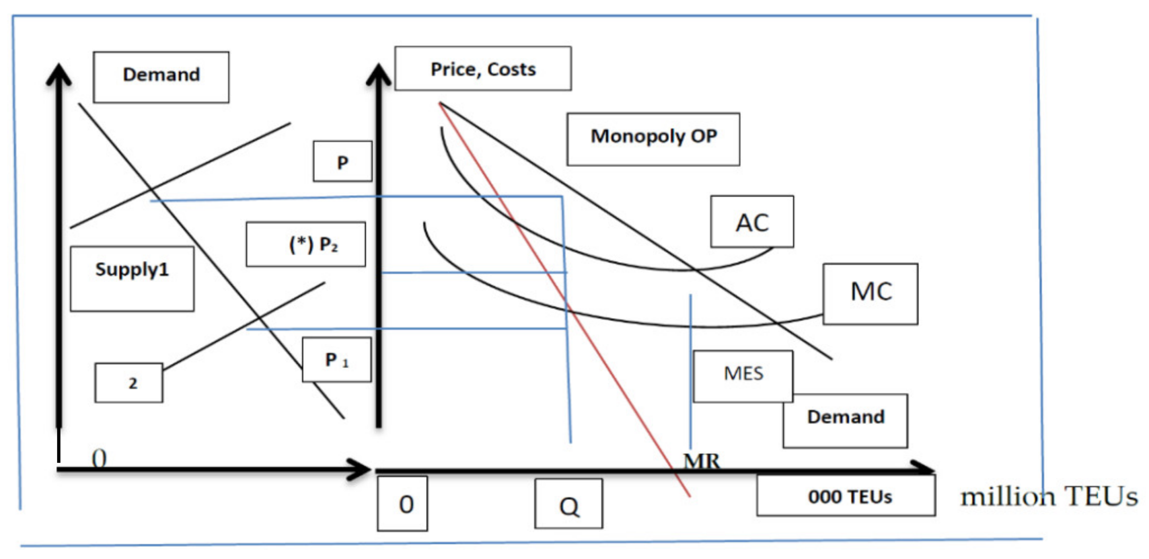
11. A Model of Oligopoly66 and… Competition

The model presented in this paper (Figure 13) is a metaphor inspired by “monopoly” theory. There are a number of top firms67, referred to here as ‘leaders’. Leaders face little competition in their market. The competition comes from smaller, fringe firms, which collectively account for no more than 30% to 40% of the market. Fringe firms do not threaten the market shares of oligopolies. Oligopolies68 have together a 60% to 70% market share. Fringe firms are price takers.
In CM, 9 containership companies are oligopolies, and earned $121b (2008), from an aggregate total share of fleet capacity 64%: AP Moller-Maersk, CMA CGM, Hapag-Lloyd, APL, Hyundai, (Hanjin), NYK, CSAV, and Zim69. They have a 71% share of total revenue (59% in TEUs carried). In May 2008, the 9 top companies had a share in the existing fleet of 69.4% (Lorange 2009) in TEUs.
As shown, D1D2 is the total demand curve of shippers for containership services over one particular route. From this we subtract what is offered by the fringe firms, leaving LEHD2. Oligopolies exercise control over prices by adjusting production and with various co-operations, surcharges, negotiations and GRIs, to produce OA, satisfying the greater part of total demand: i.e., 60% (= LEHD2); also PC = EF.
Fringe firms produce AB (40%). MC is assumed constant, and < AC, (AC is not shown), due to strong economies of scale. MC need not be constant for fringe firms, as shown (MC’ is rising). Oligopolies maximize profits at quantity OA, where MR = MC, and determine price at OP. They can supply the whole market, if fringe firms do not. The price OP is lower than the monopoly price. The smaller carriers take the price OP.
Rigorously, let the demand be P = 100 ( Q d + Q f ) = 100 45 30 = 25 [1], and let supply of fringe firms be: i = 1 n Q f i = 2 ( P 10 ) , but only for P 10 [2]. MC ' = 10 + 1 / 2 Q f = 25 [3]. MR = 40 2 / 3 Q d = MC = 10 [4], and P = 25 = price, and Qd = 45 = oligopolies’ production. Substituting [2] into [1], we get P = 40 1 / 3 Q d = 25 . Oligopoly power equals to LI 0 = ( 25 10 ) / 25 = 0.6 , which is less than 1, and for fringe firms LI f ( 25 25 ) / 25 = 0 . The monopoly price is 55 and LI = 0.82 , which is less than 1, assuming MC = 10 for monopoly. However, MC must be less than that for LI to approach 1.
If the group of oligopolies reduces production by 1 unit, fringe firms supply more, by 2/3 (Martin 2010). So, fringe firms fill a gap. Fringe firms cause production to be higher than the monopoly level at 75 units (up by 30).
The AR was $2381/TEU for Hyundai (in 2008)70 over all routes. Hyundai71 was the most efficient carrier, having an LI of 0.38 (2008) and 0.46 (2009) (oligopoly), and this increased from the boom to the depression. Elasticities of demand for this company were 2.20 and 2.63 (2008; 2009), so it faced an increasingly elastic demand. The 9-member oligopoly group, on average, obtained $1835/TEU. The smaller competitive group obtained $872 on average over all routes. Oligopoly power72 provided an extra amount of $1509/TEU to leader73 (Hyundai). UNCTAD (2016) argued that the growing concentration may squeeze out smaller carriers, and it may result in an oligopolistic market structure.
• Alliances
Alliances (Goulielmos 2017): KHY/Ming-Hanjin and Kawasaki & Yang had a higher HHI of 1830. Alliances increase concentration. Concentration also often reached higher levels with HHI from 3035 to 6746 (monopoly), when one takes port traffic into account (as we did with 7 carriers). Also, concentration increased as carriers preferred to call where they had their own terminals.
Mergers also occurred in 2015 between China Ocean Shipping Co. and China Shipping Container Lines, and Hapag-Lloyd and United Arab Shipping Co. CMA CGM acquired Neptune Orient Lines. Moreover, the top 16 carriers joined and created 3 global alliances. Hyundai may join the alliance of Maersk and Med. in 2016. Sanchez and Mouftier (2016) estimated that the level of concentration using HHI rose by 70% between 2014 and 20016. So, depression causes firms to gather together, which is a natural reaction. Unity provides survival and increases power.

12. Conclusions

The primary problem of the CM is the imbalance between supply and demand since the end of 2008. This was coupled with shorter distances. This also led to record low levels of freight rates, containerships in lay-up, SS and (reluctant) scrapping, especially of low aged tonnage. Moreover, SS encouraged by exceptionally high fuel prices, which peaked in 2011, and by low freight rates. These are the characteristics of a depression.
What is less well-understood, however, is the oversupply of tonnage. Carriers are unable to predict demand, so they assume that demand will rise. Maritime economists are also unable to predict freight rates. Thus, carriers proceeded to order74 larger and more competitive ships. Moreover, carriers have to cut-out costs to increase operating profit. One way is to resort to economies of scale (ES). ES, however, reduce net profit, because they create increased finance costs, given that internally generated funds are limited during a depression.
The aggressive shipbuilding programs needed some $3b to $4b per company. Liner companies could pass as much as 75% of this task over to the shoulders of the independents (Seaspan, Danaos, etc.), which are more efficient. However, the problem of overcapacity remained. ES increase market share, but reduce net profits. The market share was correlated to revenue, but not correlated to net profit and operating profit. So, the right policy is to proceed to ES with internally generated funds.
Carriers also economized by cutting frequent port calls. This led to the delivery of an inferior quality of service in terms of frequency and the duration of transit. In the depression, carriers also eliminated rivals by cooperation, by mergers and acquisitions, and by sending… rival’s ships to lay-up and scrapping. Some authors have argued that this was achieved by ES. The strategy of ES leads carriers to shipbuilding yards instead of staying away75 from them. Carriers did not build so many ships in 2016 and in 2017, as in 2008 (peak), but still they have built half that amount (43.3m dwt in 2016 compared with 80m in 2008).
One should not rush to identify certain containerships as “mega”, as sizes change. In 2009 mega ships were from 12,500 to 13,300 TEUs. This tendency, which started in end 2007, will continue as ES are not exhausted (AC at minimum—MES), even with 21,000 TEUs ships. We need ships of perhaps 40,000 + TEUs for that. So, pricing on the basis of P = MR = MC given the lower AC, condemns carriers to losses. So, carriers are right to ask for frequent price adjustments so that they can equate price with AC (over time).
Theory suggests that only monopolies can change the quality of service, and it seems that maritime oligopolies can do that too, through SS.
As deliveries in 2016 were 1.69m TEUs, and the idle tonnage was 1.59m TEUs, it follows that deliveries of certain carriers probably sent rivals’ ships—in almost equal volume—to lay-up.
The larger is a new-building, the lower the cost per TEU (which is $944 for the 15,000 TEUs vessels). However, ES were not enough to balance the industry by sending rival ships to scrapping. Newer tonnage had to be scrapped an action which carriers were reluctant to. As a result, oversupply in the CM was here to stay, as at current scrapping rates it will take roughly 7 years to cope with deliveries (assuming deliveries at 2015 level).
Also, new-buildings are put on routes paying higher freight rates, such as the Transpacific (Shanghai–USEC) and Shanghai–West Africa (Lagos) markets. This is higher than average revenue for the industry’s top shipping companies of $961/TEU (in 2015) (UNCTAD 2016). Indeed, market leaders have abandoned “poor” routes, and concentrated on the most profitable76 (AP Moller-Maersk; end of 2006) to increase profits at the expense of market share.
The 3 regressions run gave unexpected signs and rather low correlation coefficients, and only showed a strong relationship between revenue and market share. This is explained, as is the link between revenue and net profit, by important intervening variables like taxation, operational costs, and finance expenses, which diminish net profits. Port and canal pricing based on size forced companies to cut both calls and passages during a depression.
Concentration, indicated by an HHI of 683 < 1000 and an oligopoly power of 0.55, which, being well below 1, does not support the conclusion that CM is an oligopoly as a whole. However, there is an oligopoly made up of market leaders, when their markets are properly defined and the competitive fringe firms are examined separately. A mixed model of oligopolies and competitive (fringe) firms exists in the CM.

Conflicts of Interest

Author declares no conflicts of interest.

Appendix A. Lerner’s index

Lerner, A.P. wrote an article in LSE’s journal: the “Review of Economic Studies” in June 1934 (Vol 1, No 3) titled: “The concept of monopoly and the measurement of monopoly power”, (pp. 157–75). Lerner had the bad luck for the classical books of E Chamberlin and J Robinson to appear in 1933, when the major part of his article was already written. Lerner argued that if the AC curve is horizontal, the ratio of monopoly revenue to total receipts coincides exactly with the ratio of the divergence of price from MC to price: then LI = Price-marginal cost/price [1]. If MC = marginal receipts (in equilibrium), then MR = P ( 1 1 / e ) [2] and e = P / ( P MR ) [3] and [1] becomes identical with the inverse of the elasticity of demand, if MR = MC (a special case); where e = elasticity of demand.

References

  1. Bae, Min Ju, Ek Peng Chew, Loo Hay Lee, and Anming Zhang. 2013. Container transshipment and port competition. Maritime Policy & Management 40: 479–94. [Google Scholar]
  2. Baumol, William J., John C. Panzar, and Robert D. Willig. 1982. Contestable Markets and the Theory of Industrial Structure. New Yore: Harcourt Brace Jovanovich. [Google Scholar]
  3. Besanko, David, David Dranove, Mark Shanley, and Scott Schaefer. 2013. Economics of Strategy, 6th ed. Hoboken: Wiley. [Google Scholar]
  4. Borenstein, Severin. 1989. Hubs and high fares: Dominance and market power in the US Airline industry. Rand Journal of Economics 20: 344–65. [Google Scholar] [CrossRef]
  5. Chamberlin, Edward H. 1933. The Theory of Monopolistic Competition. Cambridge: Harvard University Press. [Google Scholar]
  6. Cullinane, Kevin, and Paul Tae-Woo Lee. 2002. Contemporary research in global shipping and logistics. Maritime Policy & Management 29: 203–8. [Google Scholar]
  7. Dixit, Avinash. 1979. A model of duopoly suggesting a theory of entry barriers. Bell Journal of Economics 9: 1–17. [Google Scholar] [CrossRef]
  8. Drewry Shipping Consultants Ltd. 2010. Container Forecaster, 2Q 2010, Quarterly Forecasts of the Container Market. London: Drewry Shipping Consultants Ltd. [Google Scholar]
  9. Ducruet, César, Theo Notteboom, Daniele Ietri, Arnaud Banos, and Céline Rozenblat. 2010. Structure and dynamics of liner shipping networks. Paper presented at IAME Conference, Lisbon, Portugal, July 7–9. [Google Scholar]
  10. Ferrari, Claudio, Francesco Parola, and Alessio Tei. 2015. Determinants of slow steaming and implications on service patterns. Maritime Policy & Management 42: 636–52. [Google Scholar]
  11. Furuichi, Masahiko, and Natsuhiko Otsuka. 2015. Proposing a common platform of shipping cost analysis of the Northern Sea Route and the Suez Canal Route. Maritime Economics & Logistics 17: 9–31. [Google Scholar]
  12. Fusilo, Mike. 2003. Excess capacity and entry deterrence: the case of ocean liner shipping markets. Maritime Economics & Logistics 5: 100–15. [Google Scholar]
  13. Gharehgozli, Amir, Joan P. Mileski, and Okan Duru. 2017. Heuristic estimation of container stacking and reshuffling operations under the containership delay factor and mega-ship challenge. Maritime Policy & Management 44: 373–91. [Google Scholar]
  14. Goulielmos, Alexander M. 2017. Containership market: A comparison with Bulk Shipping & a proposed Oligopoly model. SPOUDAI-Journal of Economics and Business 67: 47–68. [Google Scholar]
  15. Hirshleifer, Jack, and Amihai Glazer. 1992. Price Theory and Applications, 5th ed. Upper Saddle River: Prentice Hall Int., ISBN 0-13-721671-8-p. [Google Scholar]
  16. Holloway, Stephen. 2003. Straight and Level: Practical Airline Economics, 2nd ed. Farnham: Ashgate. [Google Scholar]
  17. Jacobson, David, and Bernadette Andréosso-O’Callaghan. 1996. Industrial Economics and Organization: A European Perspective. London: McGraw-Hill, ISBN 0-07-707889-6. [Google Scholar]
  18. Koopmans, Tjalling Charles. 1939. Tanker Freight Rates and Tankship Building. Haarlem: De Erven F. Bohn. [Google Scholar]
  19. Kou, Ying, and Meifeng Luo. 2016. Strategic capacity competition and overcapacity in shipping. Maritime Policy & Management 43: 389–406. [Google Scholar]
  20. Lam, Jasmine S. L., Wei Yim Yap, and Kevin Cullinane. 2007. Structure, conduct and performance on the major liner shipping routes. Maritime Policy & Management 34: 359–81. [Google Scholar]
  21. Lin, Dung-Ying, Chien-Chih Huang, and ManWo Ng. 2017. The coopetition game in international liner shipping. Maritime Policy & Management 44: 474–95. [Google Scholar]
  22. Lorange, Peter. 2009. Shipping Strategy: Innovating for Success. Cambridge: Cambridge University Press, ISBN 978-0-521-76149-9. [Google Scholar]
  23. Maloni, Michael, Jomon Aliyas Paul, and David M. Gligor. 2013. Slow steaming impacts on ocean carriers and shippers. Maritime Economics & Logistics 15: 151–71. [Google Scholar]
  24. Martin, Stephen. 2010. Industrial Organization in Context. Oxford: Oxford University Press, ISBN 978-0-19-929119-9. [Google Scholar]
  25. Munim, Ziaul Haque, and Hans-Joachim Schramm. 2016. Forecasting container shipping freight rates for the Far East-Northern Europe trade lane. Maritime Economics & Logistics 19: 106–25. [Google Scholar]
  26. Niamié, Octave, and Olivier Germain. 2014. Strategies in Shipping Industry: A Review of “Strategic Management” Papers in Academic Journals. ESG UQAM. Quebec City: University of Quebec. [Google Scholar]
  27. Notteboom, Theo E. 2002. Consolidation and contestability in the European container handling industry. Maritime Policy & Management 29: 257–69. [Google Scholar]
  28. Reid, Walter, and David Roderic Myddelton. 2005. The Meaning of Company Accounts, 8th ed. Gower: Gower Pub Co., ISBN 0-566-08660-3. [Google Scholar]
  29. Robinson, Joan. 1933. The Economics of Imperfect Competition. London: Macmillan. [Google Scholar]
  30. Sanchez, Ricardo, and Lara Mouftier. 2016. The Puzzle of Shipping Alliances in July, 2016. Port Economics. Bergamo: IAME. [Google Scholar]
  31. Song, Dong-Wook, and Photis M. Panayides. 2002. A conceptual application of cooperative game theory to liner shipping strategic alliances. Maritime Policy & Management 29: 285–301. [Google Scholar]
  32. Spence, A. Michael. 1977. Entry, capacity, investment and oligopolistic pricing. Bell Journal of Economics 8: 534–44. [Google Scholar] [CrossRef]
  33. Strandenes, Siri Pettersen. 2012. Maritime Freight Markets. In The Blackwell Companion to Maritime Economics, 1st ed. Edited by Wayne K. Talley. Hoboken: Blackwell Publ. Ltd. [Google Scholar]
  34. Sys, Christa. 2009. Is the container liner shipping industry an oligopoly? Transport Policy 16: 259–70. [Google Scholar] [CrossRef]
  35. Sys, Christa, Hilde Meersman, and Eddy Van De Voorde. 2011. A non-structural test for competition in the container liner shipping industry. Maritime policy & Management 38: 219–34. [Google Scholar]
  36. Train, Kenneth E. 1991. Optimal Regulation: The Economic Theory of Natural Monopoly. Cambridge: The MIT Press, ISBN 0-262-20084-8. [Google Scholar]
  37. The United Nations Conference on Trade and Development (UNCTAD). 2016. Maritime Transport Review. Geneva: UNCTAD. [Google Scholar]
  38. US Department of Justice. 2006. The Herfindahl-Hirschman Index. Available online: www.usdoj.gov/atr/public/testimony/hhi.htm (accessed on 20 September 2017).
  39. Wang, Shuaian, Zhiyuan Liu, and Xiaobo Qu. 2017. Weekly container delivery patterns in liner shipping planning models. Maritime Policy & Management 44: 442–57. [Google Scholar]
1
A branch of maritime microeconomics covering ports, ships, and shipbuilding.
2
Sys (2009) mentioned four sources (1991–2003). The last one, in 2003, was from the Japanese shipowners association: “Comments on consultation paper of council regulation 4056/1986” http://www.jsanet.or.jp/e/.
3
Game theory applied to industrial organization by Spence (1977) and Dixit (1979) to model the conduct of firms. By 1996 appeared in almost all journals. In 2002 appeared in maritime journals. It also appeared in IAME conferences since 1999 (Halifax; Santiago de Chile; Taipei). Kou and Luo (2016) mentioned another 6 maritime papers and one PhD (in Singapore)—between 1989 and 2013—using game theory; one appeared also in maritime journals (Fusilo 2003).
4
This lower quality understood by certain carriers, who tried to preserve regularity by bypassing smaller ports and/or by adding additional ships (e.g., COSCO).
5
Structure-conduct-performance.
6
On: “Transpacific”; “Europe-Far East” and “Trans-Atlantic” trade routes.
7
A.P. Moller-Maersk tried (end-2006) to boost profitability, at the expense of a larger market share, abandoning a “Transpacific” route (Lorange 2009). Many liner operators did this. The “Far East–Europe” route was considered most profitable.
8
Goulielmos (2017) confirmed this.
9
Fewer calls indicate higher concentration over ports; this is shown by “port production” per carrier (Goulielmos 2017).
10
Maersk Line stated that the fuel cost represented 50% of the total in May, 2008, while a few years prior, this was only 10% (Lorange 2009).
11
Average freight rates fell, after April 2008, from a high ~$1700 to ~$1400 in April 2009 for Trans-Atlantic; from ~ $1550 to ~$1100 for Transpacific and from ~$1400 to ~$1180 for Far-East–Europe (Ferrari et al. 2015).
12
One should not be surprised by lower profits given the rationality of game theory (prisoner’s dilemma).
13
This is a “cooperative competition” based on game theory (J.F. Nash in 1944).
14
It started this strategy with the 3E https://www.maersk.com/en/explore/fleet/triple-e, Evergreen, 2008.
15
Seaspan ordered 42 containerships in 2008 of an estimated value of $3.9b, at higher prices. Other independents were: Peter Dohle, MPC Group, C.P. Offen, Nord capital, B. Rickmers, and others.
16
The motives of Independents were: to expand fleet, have a steady cash flow, and achieve advantageous finance terms (from lenders and equity markets) (Lorange 2009).
17
18
On data available. Term used by UNCTAD.
19
Given that the liner freight rate was ~10%—on average—on the value of cargo transported, carriers should have earned €684b revenue in 2015. This % has been calculated from data coming from UNCTAD on ratios of liner freight rates to prices of about 10 selected commodities in 1975, 1990 and 2015. The €/$ exchange rate at the end of 2014 was 1.21.
20
According to our experience from bulk trades a shipowner needs a maximum of 3 years to be convinced to lay a ship up.
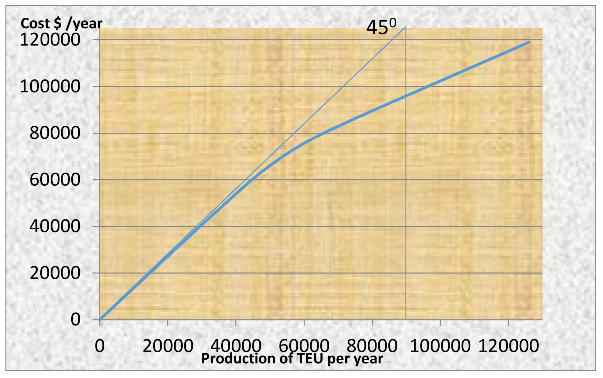
21
Marginal cost is calculated by dividing the rise in total cost by additional production (TEUs).
22
23
Data from UNCTAD (2016).
24
Through ‘capacity control’, and/or cost advantage.
25
26
A capital cost of $159.4m is calculated by Furuichi and Otsuka (2015) per year at an interest rate 7% over 15 years for a ship of 15,000 TEUs.
27
Fuel consumption per distance unit is proportional to the sailing speed squared (Furuichi and Otsuka 2015).
28
Port dues etc., historically, conceived in a partnership understanding that ports contribute to ships’ revenue, so they are entitled to withhold part of it by setting port rights on volume. Volume of cargo was, historically, determined by GRT, later by NRT, and even later by GT, and in certain ports in France by dwt. NRT replaced GRT, as the former includes ship’s closed spaces that bring-in nothing. Moreover, dwt includes bunkers, water etc., which too bring no revenue, but they represent a cost. Boxes, we believe, should pay port dues on their content value. The recent move of IMO (*) to know box weight may help, if it is extended to the value of the contents of the box. (*) On 1 July 2016, in SOLAS, there was an amendment for the mandatory verification of the gross mass of containers. Certain ports have recognized this issue and provided volume discounts in confidential contracts. However, our contribution is to put this matter in a way that will persuade ports to revise port expenses etc., to encourage ship sizes to become bigger.
29
Ship’s size entails certain costs for ports: longer quays, deeper draft, more spacious yards etc. The new ‘charging port policy’—favoring size—can be designed to make transshipment redundant, we believe.
30
Density matters because of fixed costs. These are the ruthless enemy of firms; it is the cost that is insensitive to the level of production, and it must be paid, even when production is nil. Certain industries have high fixed costs, like shipbuilding. Shipping has 50% of total costs fixed (mainly in new buildings). Fixed costs can be made more sensitive to production by reducing AFC-average fixed costs. The enemy of fixed costs is economies of scale.
31
Hurdle et al. in 1989, quoted by Jacobson & Andréosso-O’Callaghan, op.cit. Holloway (2003).
32
E.g., “low-cost” airlines. Borenstein (1989) found that monopoly routes had higher fares. However, contestability was not responsible for the competitive rates, as believed, but only for lower ones. A CM company can exit from a trade route, but remain in the market. Contestability has to be sought after within a trade route.
33
This ended the exemption of liner conferences from EU competition rules (EU CR 4056/1986).
34
In the Europe-Far East route, CR4 was 40% in 2002; 52% for Transatlantic. Some argue that concentration has no important effect on high prices, and the sharpest increase occurs at a concentration ratio ≥50% (Martin 2010).
35
Maersk = 15.15%; Med. Ship. Co = 13.4%; CMA CGM = 9.22% and China Ocean Ship. (Group) Co = 7.83%.
36
This is based on the market shares (%) of the 50 leading liner shipping companies in total shipboard capacity deployed in TEUs (UNCTAD 2016). The CR4,1998–2002—in slot capacity—found (rounded) (Lam et al. 2007): 43% (1998), 43% (2000), and 41% (2002) in Transpacific; 37%, 43%, and 39.5% in Europe–Far East; and 44%, 45.5%, and 52% in Transatlantic. So, Transatlantic should have higher freight rates, due to higher concentrations among the 3 main traders, but this did not happen, as between 1998 and 2002, Transpacific (eastbound, but not westbound) achieved the higher freight rates among all trades: $1400; $2200; $1500.
37
38
In 5 US industries, in 1986, the CR4 varied from 62% to 93%.
39
Geithman-Marvel and Weiss in 1981, quoted by Hirshleifer and Glazer (1992).
40
Concentration in CM is not continuous.
41
During a depression expenses should be reduced, showing also the efficiency of carriers.
42
Exceptions are the firms: CPS; and PON (PONL) and APL, which had losses.
43
CPS (CP ships) had 18.5% (high) in CR4 in Transatlantic in 2002, and ‘net profit’ of only 1.93% or $52m on a $2.7b turnover…
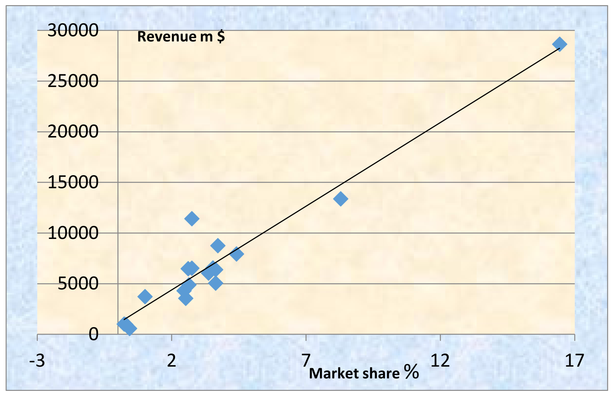
44
Pearson product-moment coefficient of correlation: r = xy nx mean y mean / n σ x σ y . The 14 carriers presented (Figure 9a) belong to a group of 16 ‘major’ carriers having ~$55b turnover in 2002, perhaps 25% of total. The coefficient does not indicate also causality, but only a degree of association between the two variables.
45
The Transpacific eastbound, in 4th quarter 1999, provided a freight rate of $2200/TEU; Transpacific westbound paid $710.
46
Besanko et al. (2013) argued that a necessary first step in identifying monopolies is the ‘market definition’ or ‘competitor identification’. The US Dept. of Justice argues that if a merger among competitors would lead to a small (say 5–10%), but significantly non-transitory (12 months at least), increase, in price, and then this market is well defined. This is known as the “SSNIP” criterion; Martin (2010).
47
Chamberlin (1933) and Robinson (1933) were dissatisfied with the two polar cases of monopoly and perfect competition as a description of reality (Appendix A).
48
Sys et al. (2011) using an unbalanced panel of data of a sample of 18 major liner operators (1999–2008) rejected the: neoclassical monopoly, collusive oligopoly or the conjectural variations of short-run oligopoly by the power of the “Panzar & Rosse H-statistic” in 1987. It suggests that the CM operates in a monopolistic competitive environment…
49
The CR4 for liner companies in slot capacity increased from 24% in 2000 to 39% in 2009; this remained steady after 2006, at 38–39%, till 2009 (Sys 2009).
50
CR4,2007: Transatlantic/eastbound ~61%; India–US ~63%; Med–North America ~66% (eastbound); US–India ~62%; North America–Latin America (Southbound.) ~70%; US–M East ~69% and M East–US ~84%. So, trade lanes reveal true concentration.
51
HHI < 1000 indicates no concentration; from 1001 to 1799 shows a moderate one; from 1800 and over shows high concentration.
52
The index is named after (Orris) Herfindahl, and this is a product of his doctoral thesis for steel industry at Columbia University. It is also named after Hirschman; so the index frequently is denoted by HHI. In fact there is a dispute of who is the father of the index.
53
54
Sys (2009) found HHI2009~575 for liner total in slot capacity and CR4~39%. For total turnover she found CR4,2006 = ~50%. Lam et al. (2007) found in Transpacific HHI1998–2002: 703; 650; and 646 (rounded); in Europe–Far East: 577, 666, and 644; and in Transatlantic: 674, 780, and 891.
55
Taking revenue of 38 carriers in 2008; taking 24 carriers, the HHI2009–2010 increased to 1609 and 1777.50; 29 carriers had HHI = 1132 (2008). Data: from Drewry Shipping Consultants Ltd. (2010).
56
According to Besanko et al. (2013).
57
Our assumption is that if $1449 = price; then $1449 − $645.50/$1449 = LI = 0.5545. MC = $645.50.
58
Shanghai to N Europe-S America (Santos)-Australia/New Zealand (Melbourne).
59
Container freight markets and rates, 2009–2015, found in UNCTAD (2016), are taken as prices.
60
In CM we cannot rely on the equality of LI to inverse of elasticity of demand due to existing disequilibrium.
61
Firms that pursue economies of scale, approaching their MES—say at 40,000 TEUs ships—create a cost advantage over smaller ones.
62
Proof: MR = P + Q dP / d Q ; dividing by P, then MR / P = ( 1 + Q / P × dP / d Q ) = 1 + 1 / e d , as e d = dP / d Q × P / Q , or MR = P ( 1 + 1 / e d ) , or MR = P ( 1 1 / | e d | ) .
63
Sys (2009) found that the “instability index” is closer to 0 than to 1, meaning a relatively stable competition between 2000 and 2005, but not in 2006.
64
Proof: PCM = ( P M C ) / P , P ( PCM ) = P M C and M C = P ( 1 1 / e d ) : replacing P ( PCM ) = P P ( 1 1 / e d ) and PCM = P / P P ( 1 1 / e d ) / P = 1 ( 1 1 / e d ) = 1 / e d .
65
One of the strange matters on this planet is the tolerance of governments of the cartel of OPEC; this is excluded because it is made up of governments.
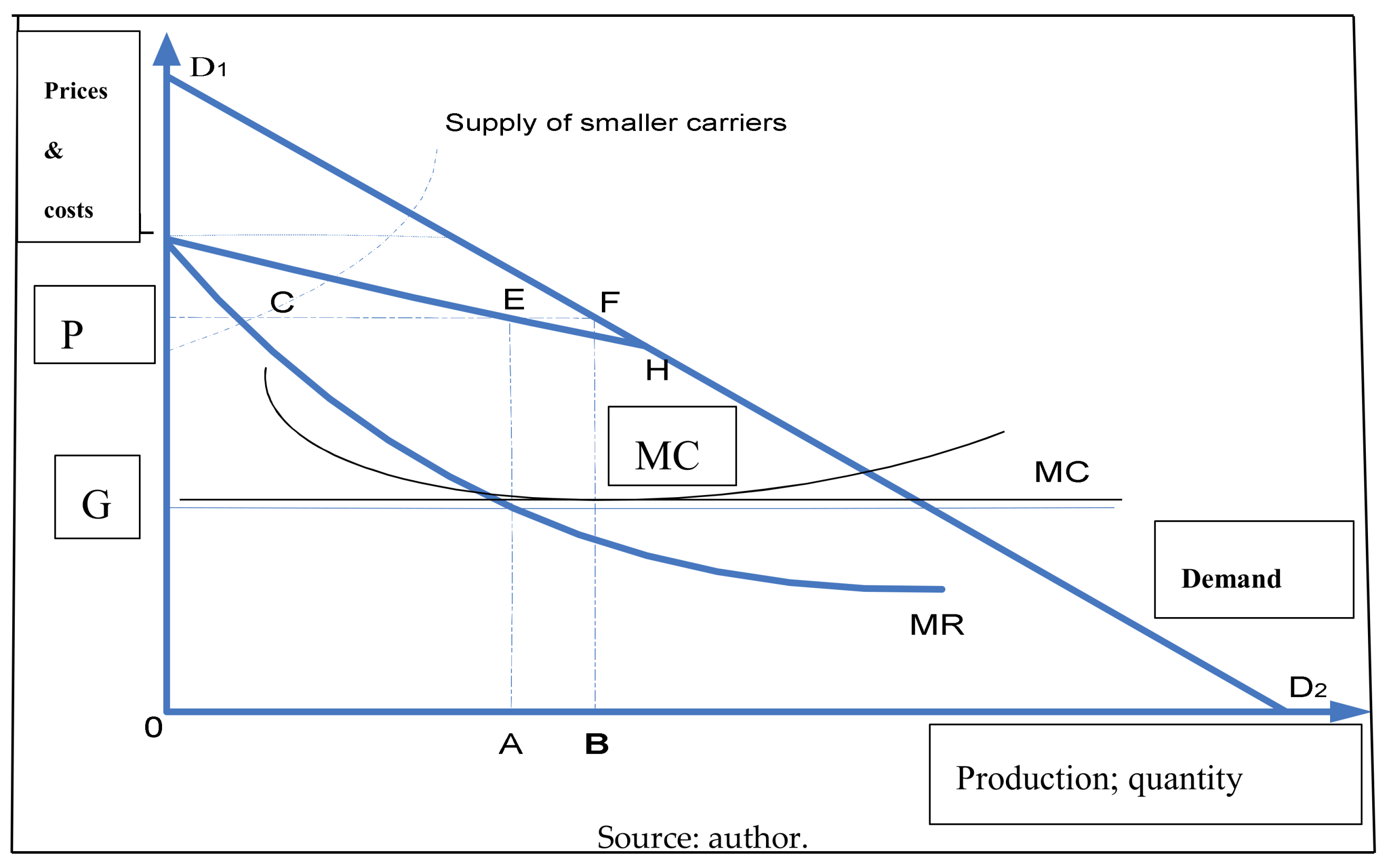
66
An earlier version is presented in Goulielmos (2017); see also: (Martin 2010, p. 213; Besanko et al. 2013).
67
Lorange (2009) also speaks of price leaders and price takers, with different roles.
68
Sys (2009), in a clearer manner, also showed two different oligopolies in 2 sub-markets, as mentioned in Table 1.
69
One may distinguish alliances among them.
70
71
Despite the 68.3% orders on existing fleet in 10 March 2008.
72
This means the ability to choose the most profitable routes, the frequency of service and to eliminate competitors etc.
73
The price-leader makes each firm give-up its pricing autonomy and passes control over group’s pricing to one single firm.
74
The 2nd half of 2007 witnessed an explosion of orders. In four months, as many ships were ordered as in the previous three years (Lorange 2009).
75
AP Moller-Maersk (end 2006) resisted the urge to the purchase of new tonnage.
76
Far East–Europe?
Figure 1. The Main Decisions taken by Carriers under end-2008 depression, 2009–2017. Source: author.
Ijfs 06 00090 g001
Figure 2. Containerships on order, 2000–2016 (000 dwt). Source: Author and excel on numbers from UNCTAD (2016).
Ijfs 06 00090 g002
Figure 3. World seaborne trade in containers: (a) in billion ton-miles, 2000–2016; and (b) in million tons loaded (1980–2015; selected years). Source: Author and excel on numbers from UNCTAD (2016). Trend line: a 2 year moving average. 2015 estimated; 2016 forecast.
Ijfs 06 00090 g003
Figure 4. Average distances prevailed in CM between 2005 and 2015. Source: Figure 3, excel and author. Trend: a two-year moving average.
Ijfs 06 00090 g004
Figure 5. Demand and supply growth rates, 2001–2016. Source: Author and excel on numbers from UNCTAD (2016); 2016 figures are projected.
Ijfs 06 00090 g005
Figure 6. (a) Capital cost, total and average cost per size, (b) AC, and MC in CM per size, 1994–2013. Source: Author, excel and numbers from Furuichi and Otsuka (2015).
Ijfs 06 00090 g006
Figure 7. Elasticity of Demand and MR (relationship) at firm’s level.
Ijfs 06 00090 g007
Figure 8. Total cost per year versus total annual production, 1994–2013. Source: Author and excel on numbers from Furuichi and Otsuka (2015).
Ijfs 06 00090 g008
Figure 9. Scatters of (a) net and (b) operating profit as % of turnover and concentration ratios CR4, and CR10 over 3 routes for 14–15 major container carriers (2002). Source: Author, regression and data from Lam et al. (2007).
Ijfs 06 00090 g009
Figure 10. Regression between revenue and market share (2008; 2010). Source: Author and excel on numbers from Sys et al. (2011).
Ijfs 06 00090 g010
Figure 11. CM industry and firm in equilibrium? (*) Oligopoly tries to achieve price OP2, after pricing at OP1, using GRIs. Source: author.
Ijfs 06 00090 g011
Figure 12. Oil prices, $ per ton, 1994–2015. Source: Author and excel, numbers from Furuichi and Otsuka (2015) and UNCTAD for 2014–2015.
Ijfs 06 00090 g012
Figure 13. A group of oligopolies and a number of fringe competitive firms in Transpacific Eastbound.
Ijfs 06 00090 g013
Table 1. Sys’ (2009) conclusions on containerized industry, 2000–2009.
Concentration49Industry’s StructureIndustry’s StructureIndustry’s Structure
The industry is increasingly concentrated; done by consolidationLoose oligopoly found in the 53% (8/15) of trade routes (2007); if CR4 = 25–60% = effective competition with a reasonably easy entryThe 7/1550 (47%) trade lanes were a tight oligopoly: CR4 > 60%; i.e., oligopoly whose market characteristics facilitate the realization of supernormal profits for a long time with high barriers to entryChain oligopoly
Given the variations in market shares, CM is neither symmetric nor asymmetric, but betweenCompetitive.
Fragmented: HHI < 1000.
Stable competition
Firms belong to oligopolistic sub-groupsA trend towards a tacitly collusive market with important operational agreements

