Abstract
This study aims to explore the relationship between economic growth, financial innovation, and stock market development of Bangladesh for the period 1980–2016. To investigate long-run cointegration, this study used the autoregressive distributed lagged (ARDL) bounds testing approach. In addition, the Granger-causality test is used to identify directional causality between research variables under the error correction term. Study findings from the ARDL bound testing approach confirm the existence of a long-run association between financial innovation, stock market development, and economic growth. Furthermore, the findings from the Granger-causality test support bidirectional causality between financial innovation, economic growth and stock market development, and economic growth both in the long run and short run. These findings support the theory that market-based financial development and financial innovation in the financial system can spur economic development.
JEL:
O47; P34; D53; 053
1. Introduction
Developmental economic theory emphasizes the efficient mobilization of economic resources in the economy because the optimal mobilization of economic resources transforms national saving into a productive investment, which eventually leads to sustainable economic growth. Empirical studies, therefore, pay attention to investigating the causality between savings and investment [see, for example, (Geiger 1960; Soyode 1990; Aigbokhan 1995; Huntington 1993)]. The mobilization of economic resources immensely depends on the financial intermediation process in the financial sector, which implies that a well-functioning financial sector not only expedites efficient mobilization of economic resources but also plays a fundament role in economic growth as well (Gurley and Shaw 1955).
Not surprisingly, over the last decade, the financial development and economic growth nexus has drawn immense attention among researchers and policymakers from both the developed and developing countries. A number of studies have been conducted to investigate different proxy variables of financial development and empirical studies have confirmed the positive association between them [see, for example, (Azam et al. 2016; Bwirea and Musiime 2015; Chang and Caudill 2005; Comin and Nanda 2014; De Gregorio and Guidotti 1995; Kassimatis 2000; Kyophilavong et al. 2016; Ram 1999; Hasan and Barua 2015; Saad 2014; Shahbaz et al. 2015)]. The contribution of financial development towards economic development comes with either bank-based financial development, market-based financial development, or both. Different countries experience financial development in both or either way.
For about a century the controversy over whether the financial market contributes to economic development has been ongoing. The financial market contribution was appreciated in regards to capital formation and productive investment. Efficient financial markets play a fundament role through pooling savings and mobilizing funds into productive investments (Bekeart and Harvey 1997), promoting domestic capital formation (Nazir et al. 2010), encouraging savings by offering diversified investments (Bayar 2016), and support increase financial efficiency in turn, thus fostering economic growth. Market-based financial development, therefore, becomes a fundamental determinant for economic growth either directly or indirectly, which induces researchers and academics to explore nexus stock market development-led economic growth (see for example, King and Levine 1993; Enisan and Olufisayo 2009; Nyasha and Odhiambo 2016; Pradhan et al. 2015; Bayar 2016).
The well functioning financial market, both the money market and capital market, immensely influence the financial development process with optimal allocation, diversified investment opportunities (Wong and Zhou 2011), and capital allocation efficiency in the financial system. Furthermore, the development of financial market derived financial innovations in the economy changes with technological, creating greater efficiency in the financial institutions, which can then offer better financial products and services (Bilyk 2006; Ajide 2015; Nagayasu 2012). Evolvement of the financial market in the economy permits investors to accumulate funds and encourage savings propensity in the economy by offering various financial instruments and a reduction of investment risk through diversification. Capital markets, moreover, not only promote capital accumulation but also encourage saving propensity in the economy for future investment, eventually leading to economic growth.
Financial development can be accelerated by encouraging financial innovation in the economy. This is because financial innovation brings changes to the financial system, such as diversified financial services in the banking sector and a reduction of investment risk through the incorporation of financial instruments in the capital market (Handa and Khan 2008; Djoumessi 2009; Simiyu et al. 2014). Over the last decade, the financial sector of Bangladesh has passed through some financial reform strategies that have created an efficient financial sector with efficient financial institutions and a capital market. The financial system of Bangladesh is predominated by a banking industry that accounts for 65% of the total financial assets of the financial system (Bangladesh Bank 2017). Financial institutions, especially private commercial banks, play a fundamental role in financial progress by innovating various financial goods and services in the financial system. Eventually, these goods and services expedite steady economic growth in the long run. On the other hand, the capital market has emerged as a source of long-term capital since incorporation; market capitalization to GDP was 21.45% in 2016, and the average growth rate was 15% (Bangladesh Bank 2017). For ensuring long-term capital accessibility, the government implemented initiatives for potential equity issuance, moreover, Bangladesh, over the period, experienced steady economic growth of around 6.5% on GDP. Such progress is evidence of a concerted effort from every sector of the economy.
With this research, we intend to explain the association and causality between financial innovation, stock market development, and economic growth in Bangladesh. The novelty of this research is; (1) we consider a longer period series of data, from 1980 to 2017. A few empirical studies have focused on the nexus between the financial development and economic growth of Bangladesh within this limited period. (2) We are using a newly developed autoregressive distributed lagged (ARDL) bound testing approach proposed by Pesaran et al. (2001) to investigate the cointegration between financial innovation, stock market development, and economic growth. We also investigate directional causality by applying Granger causality under an Error Correction Model (ECM). The remaining section of this paper proceeds as follows; Section 2 provides a theoretical and empirical analysis of financial innovation, stock market development, and economic growth. Detailed variables and the definition of the research methodology are explained in Section 3; Section 4 represents the model findings, and interprets them. Section 5 presents the research findings with policy implications for future development.
2. Literature Review
Sustainable economic growth requires capital accumulation for investment and efficient mobilization of economic resources in the economy. Financial institutions and financial markets play a fundamental role in the facilitation of a financial transaction (Seven and Yetkiner 2016). Over the period, researchers explored the impacts of financial development on economic growth considering either market-based financial development or bank-based financial development. A group of researchers argue and emphasize that market-based financial development requires an efficient stock market, this allows for the diversification of risk in investments with an efficient mobilization of capital among economic agents [see for example, (Antonios 2010; Nazir et al. 2010; Owusu and Odhiambo 2014)].
2.1. Studies on Financial Innovation and Economic Growth
The interaction of innovations in both the financial sector and the real sector provides a wave of economic growth (Schumpeter 1911). Innovation, therefore, in the economy treated as the drive of improving productivity accelerates the process of economic growth (Silve and Plekhanov 2014). Innovation can happen in the economy. Focusing on various aspects of the economy, innovation surrounding the financial system boosts the financial development process and this is known as financial innovation. Innovation in the financial sector not only accelerates financial development processes but also assists in capital accumulation (Ansong et al. 2011) and expedited technological innovation, which eventually leads to sustainable economic growth in the long run (Chou and Chin 2011; Orji et al. 2015).
Financial innovation is an integral part of economic activity with various aspects. Over the past decade financial innovation has brought structural changes to the financial system through improvement in financial institutions, service, and modified payment systems (Boot and Marinc 2010; Michalopoulos et al. 2011; Sekhar and Gudimetla 2013; Simiyu et al. 2014; Odularu and Okunrinboye 2008). Furthermore, financial innovation also assists in changing governmental regulations and shifting social attitudes towards financial development (Mwinzi 2014; Wachter 2006), which allows the financial sector to produce more effective and efficient ways to maximize economic resources in productive ways. Economic theory emphasizes that the maximization of the scarcity of economic resources from productive investment can achieve the sustainable economic development of the economy. Finance researchers including, Epstein (1992); Glaeser et al. (2004); Ozturk and Acaravci (2010), and Ansong et al. (2011) explain that efficiency in the financial sector influence by financial innovation, especially institutional innovation, expands the area of financial services in the economy by allowing a greater number of people into the mainstream economy and transforming economic resources into productive investments following maximization.
The effect of financial innovation in the financial system is versatile and diversified, including better financial services (Schrieder and Heidhues 1995; McGuire and Conroy 2013), smooth financial intermediation (Ozcan 2008; Allen 2011; Shaughnessy 2015), and better payment mechanisms (Sabandi and Noviani 2015; Blair 2011). The role of financial development in financial innovation also addresses empirical studies. Levine (1997), Jedidia et al. (2014), and Simiyu et al. (2014) explore the contribution of financial innovation to stock market developments through capital liquidation offerings. Furthermore, in their respective studies, Johnson and Kwak (2012), Odularu and Okunrinboye (2008) urge financial innovation in a domestic and international role with the easing of financial transactions. They imply financial innovation transforms a static economy to a dynamic one through capital formation, encouraging private investment, financial intermediation, and a higher level of saving propensity. In turn, a higher level of economic growth can be achieved.
The efficient financial system is the prerequisite for a modern economy because a sound and refined financial system encourages the efficiency of investment and economic growth in a market economy (Saqib 2015). The efficient financial system is the collection of financial markets, institutions, instruments and regulations that organize economic activity through productive investment (Mannah-Blankson and Belnye 2004) and expedite economic growth by creating financial opportunities (Beck et al. 2016; Chou 2007). Financial innovation in the financial system bring diversified financial products for investment purposes, and such diversity reduces the level of risk substantially, which produces more satisfaction among customers (Djoumessi 2009; Simiyu et al. 2014).
The prime focus of financial innovation is to make financial intermediation processes effective and efficient. Efficient financial intermediation enhances economic activity by providing better financial support in trade and commerce. In a study, Shittu (2012) pointed out that efficient financial intermediation has a positive impact on the economy. Efficient intermediation channels economic resources in the economy with efficiency (Cheng and Degryse 2014). A robust and efficient financial system promotes growth by reallocating economic resources in the economy effectively and efficiently. The efficient Financial system is the outcome of continuous financial innovation, which allows for the emergence of various financial institutions, especially banks, that can offer improved and better financial services with more credit facilities and financial instruments in the economy, which leads to economic growth.
2.2. Studies on Stock Market Development and Economic Growth
In their pioneer study, Gurley and Shaw (1955) explained that a developing country’s financial system is more effective for economic growth compared with less developed countries. Study findings proposed a theoretical framework that well-developed financial markets in the financial system can contribute capital accumulation by extending credit facilities to invest in projects for economic growth. The proposed stock market causes empirical studies to support economic growth (see for example, Seven and Yetkiner 2016; Wong and Zhou 2011; Jedidia et al. 2014; Smaoui and Nechi 2017; Pradhan et al. 2014a; Bayar 2016; Ake and Ognaligui 2010).
Stock market development, especially in developing countries, represents alternative sources of finance. This is because capital flow from the capital market promotes long-term investment while the banking industry tends to offer short or medium term financing rather long-term financing for investment in the economy (Nowbutsing and Odit 2009; Bencivenga and Smith 1991; Demetriades and Luintel 1996; Moldovan 2015). Among all other participants, in the financial development process, the stock market plays a major role in accelerating financial innovation and capital allocation (De Gregorio and Guidotti 1995). The development of the capital market ensures liquidity for investment (Abdul-Khaliq 2013; Ogunmuyiwa 2010), access to productive investment (Carp 2012), investment diversification (Błach 2011), and market capitalization (Saqib 2013). The emergence of an efficient stock market in the economy is inevitable to capital adequacy for long-term investment, which expedites the economic development process both in the short term and the long run. In the modern economy, an efficient capital market is considered a prerequisite towards sustainable economic growth because it allows not only a domestic capital accumulation process but also encourages foreign portfolio investment (Ishioro 2013; Masoud 2013; Caporale et al. 2003; Silva et al. 2018).
2.3. Financial Innovation and Stock Market Development
The development of the stock market is inevitable for sustainable financial development and eventually accelerates economic growth. There is a firm consensus for a well-functioning financial market, in particular, the stock market, which exploits economic potential while channeling a substantial amount of capital flow into the economy. Capital accumulation, according to Craig et al. (2008), through stock market development requires diversified investment opportunities, which appeal not only to large investors but also to small investors.
The depth and breadth of the financial market positively influences the availability of financial assets in the market along with investor’s preferences towards the diversification of investment. Financial innovation expands a financial market’s operational activities with the emergence of stock markets, derivatives securities, and diversified financial instruments covering both equity and debt instruments (Akhavein et al. 2001). The role of financial innovation in financial market development, especially for stock market development, is appreciated across the world with valuable service to financial markets including derivatives for risk management, institutional efficiency, and services with minimal cost (Juhkam 2003).
Financial markets play a critical role in mobilizing savings, evaluating projects, managing risk, monitoring managers, and facilitating transactions. Therefore, the development of financial markets is critical for a nation’s innovation (Schumpeter 1911). Existing finance scholars including Hellwig (1991); Weinstein and Yafeh (1998); and Morck and Nakamura (1999) advocate for financial innovation in the financial system and introduce a new avenue for financial market development by offering credit instruments, debt contracts, and opportunities for small investors.
Financial innovation, in the positive sense of the word, can be regarded as any new development in the financial system that either enhances its capital-allocation or operational efficiency (Kothari 2006). However, financial innovation often is driven by risk/return incentives at the level of the individual trader, structured financier, or institution. Financial innovation is truly welfare enhancing if it brings about a reduction in the cost of capital without a commensurate increase in systemic risk. The benefits of relatively broad and deep capital markets, complemented by an active derivatives market, can be measured using factors such as lower pricing, reduced cost of capital, mitigated risk exposures, broader access to capital and increased liquidity, among others.
3. Conceptual Development and Proposed Hypothesis
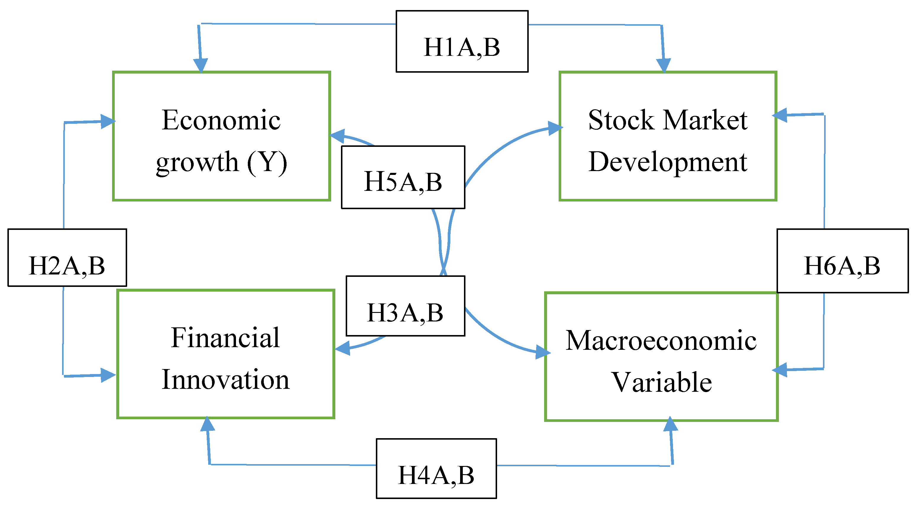
The underlying idea of this paper is to investigate the existing relationship between economic growth, financial innovation, and stock market development, along with four other macroeconomic variables. With the understanding of existing empirical studies, to assess the directional causality between variables, we perform a Granger causality test under the Error correction term. We test the following six hypotheses:
Hypothesis H1A,B (H1A,B).
Financial innovation Granger-cause economic growth and vice versa.
Hypothesis H2A,B (H2A,B).
Stock Market Development Granger-cause economic growth and vice versa.
Hypothesis H3A,B (H3A,B).
A macroeconomic variable Granger-cause economic growth and vice versa.
Hypothesis H4A,B (H41A,B).
Financial innovation Granger-cause Stock market development and vice versa.
Hypothesis H5A,B (H5A,B).
Financial innovation Granger-cause a macroeconomic variable and vice versa.
Hypothesis H6A,B (H6A,B).
Stock market development Granger-cause a macroeconomic variable and vice versa.
Figure 1 exhibits a summary of the proposed hypotheses and describes the possible causality between the variables of the study.
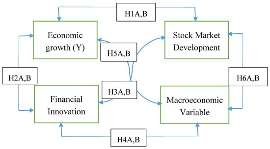
Figure 1.
A conceptual model with possible directional causality.
4. The Methodology of the Study
4.1. Variable Definition and Sources
This study uses annual time series data from 1980 to 2016. Data were collected and transformed from various sources including the World Development Indicators published by the World Bank (2017), World Economic Outlook (2017), and Statistical Hand Book 2017 published by Bangladesh Bureau of Statistics (2017). Table 1 exhibits the summary definition of research variables with expected sign in their respective coefficients in the estimation.

Table 1.
Variable definition with the expected impact.
Stock market development is the process of improvement in the financial intermediation process, quality, and quantity of stock and stock market efficiency. Capturing the stock market influence on economic growth with a single indicator is utterly impossible. However, from the existing empirical literature, we found three common indicators widely used by researchers (see, for example, Adjasi and Biekpe 2006; Bekhet et al. 2017; Demetriades and Hussein 1996; Gamolya 2006; De Gregorio and Guidotti 1995; Magweva and Mashamba 2016; Prats and Sandoval 2016; Van Nieuwerburgh et al. 2006). This present study also deploys these commonly used three indicators.
First, stock market capitalization (MC) calculated the total value of listed shares divided by gross domestic product. Researchers frequently use market capitalization to measure market size by assuming a positive correlation between market liquidity and diversification of risk.
Second, the total value traded (TAR) in the stock market as a percentage of GDP, which calculates the total value of traded security divided by GDP. This indicator is used by researchers to investigate the relationship of trading with the size of the economy, with the assumption that the market relation positively correlates with economic growth.
The third indicator for stock market development is the turnover ratio (TUR). It represents the ratio between market capitalization and total value trade in the stock market, which is significantly considered as an indicator for market liquidity position. Researchers assume a positive correlation between market liquidity with economic growth, which has been empirically tested.
There is no agreed upon measure to capture the effects of financial innovation in the economy. Furthermore, the definition of financial innovation does not specify that any particular financial changes in the financial system can be addressed as an effect of financial innovation. However, in empirical studies, scholars used various proxy indicators to capture the impact of financial innovation. Financial innovation proxy indicators include banking sector credit to private sector (GBCP) as a proportion of GDP (following Adu-Asare Idun and Aboagye 2014; Michalopoulos et al. 2009; Laeven et al. 2014) and stock of financial innovation specifying the design of intermediate goods and services in the financial system through research and development in the financial sector (Chou and Chin 2011).
Financial innovation refers to the emergence of new financial institutions and the development of new financial services and financial products. Thus a new way of financial intermediation in the financial system accelerates financial development with financial efficiency towards sustainable economic growth. Financial innovation neither limits the emergence of new financial instruments nor the introduction of new financial institutions. Financial innovation includes a broad range of innovations that cause financial developments, such as financial reporting procedure, data processing, and credit scoring, which enable financial institutions to make credit decisions. The financial intermediation process allows productive reallocation of economic resources and increases capital flow with diversified financial assets and services. To capture the financial innovation impact on economic growth, a larger number of studies repeatedly used broad to narrow money (M2/M1), where M1, known as narrow money, normally includes coins and notes in circulation and other money equivalents that are easily convertible into cash. M2 includes M1 plus short-term time deposits in banks and 24-h money market funds (see for example, Ansong et al. 2011; Mannah-Blankson and Belnye 2004; Bara et al. 2016; Bara and Mudxingiri 2016; Arrau 1991; Qamruzzaman and Wei 2017).
In this study, we also follow previous researchers and capture the financial innovation impact on economic growth, expecting a positive association.
We also chose four (04) control variables to create robustness in the model. The first control variable is gross capital formation as a percentage of GDP, with proxy of investment in the economy. Empirical studies show a positive correlation with economic growth, this is because investment fosters economic development in the economy. Hence, expect a positive sign in the coefficient.
The second control variable is Trade Openness (TO), which is calculated by adding up export and imports as a percentage of GDP. Recent empirical studies emphasize the importance of TO having a positive association with economic growth. This variable includes the study to capture the impact of trade liberalization on economic growth, expecting a positive sign in the coefficient.
The third control variable is Government final consumption expenditure (GEXP) as a proxy for government involvement in the economy for sustainable development. It signifies economic development with the assistance of infrastructural development.
The fourth control variable is Inflation, which as a proxy reports annual CPI percentage changes in the cost of average consumption for a basket of goods and services in the economy. The summary statistics and correlation matrix are reported in Table 2.

Table 2.
Summary statistics for the period (1980–2016).
4.2. The Autoregressive Distributed Lag (ARDL) Model
Several cointegration methods are available to use among those widely used methods including the residual bases Engle and Granger (1987) test, the maximum likelihood-based Johansen (1991); and the Johansen (1995) and Johansen and Juselius (1990) tests. Having a limitation with those models, in recent time, the ordinary least square (OLS) based autoregressive distribution lag (ARDL) approach become popular among researchers. The additional privilege over other cointegration methods is flexibility, this model allows a set of variables that are integrated in a different order (Pesaran et al. 2001). Moreover, a dynamic error correction model (ECM) can be derived from ARDL by using linear transformation (Banerjee et al. 1993).
This study is using the ARDL model due to the following benefits over other cointegration models. First, the autoregressive distributed lag model is superior in consideration regardless of sample size, which can be either small or finite and consist of 30 to 80 observations (Ghatak and Siddiki 2001). Second, this approach is more suitable when variables integrate in a different order, as when some variables are I(0), and some variables are I(1). Third, modeling ARDL with the appropriate lags is correct for both serial correlation and the indigeneity problem (Pesaran et al. 2001). Fourth, the ARDL model, simultaneously, can estimate long run and short run cointegration relations and provide unbiased estimation for the study (Pesaran et al. 2001). A simplified ARDL model for these variables X, Y, and Z can expressed as:
where, are long run coefficients whose sum is equivalent to the error correct term at VECM model and , , are short run coefficients. The generalized ADRL model for assessing financial innovation, stock market development impact on the economic growth of Bangladesh is as follows;
∆ indicates differencing of variables, while is the error term (white noise), and (t − 1) is for lagged period, is long run coefficient.
To capture long-run cointegration among variables, we formulate the unrestricted error correction model (UECM) under the ARLD approach considering each variable as the dependent variable to estimate the best-fitted model for further analysis as shown in matrix form.
An alternative hypothesis is:
For decision-making criteria about (H0 or H1), Pesaran et al. (2001) proposed the following procedure;
- If Fs > upper bound of critical value, confirm the existence of cointegration.
- If Fs < lower bound of critical value, conform variables are not cointegrated.
- If Fs ≤ upper bound and ≥lower bound of critical value then the conclusive decision may not reach about variables cointegration.
Once, the long run association established, the next two steps need to be executed to estimate long run and short run coefficients of the proposed ARDL models. The long-run ARDL (m, n, q, t, v, x, p) equilibrium model is as follows
The legs length of the ARDL model are to be estimated using Akaike Information Criterion (AIC). Using time series data for the study, Pesaran et al. (2001) proposed that the maximum lag length is 2. The short-run elasticities can be derived by formulating the error correction model as follows.
where the error correction term can be expressed as;
However, to investigate directional causality among variables, the following vector error correction model (Equation (6))
where, to represents constant term; to represent the short coefficients of the models; to represent coefficients of error correction term; ECT(t−1) are the long run coefficient and to represents white nose of error correction term.
5. Data Analysis and Interpretation
5.1. Unit Root Test
In econometric analysis variable order of integration is important for having internal inconsistency among the research variables. To ascertain the order of the integration, we perform the Augmented Dickey–Fuller test proposed by Phillips and Perron (1988). A stationary test with a null hypothesis non-stationary against the presence of a stationary in the dataset under three different assumptions. Furthermore, the P-P test is applied to investigate evidence of a structural break in the time series data. The results of the stationary test are presented in Table 3. Table 4 reports the unit root test assuming the single break point test of Perron (1997) and Zivot and Andrews (2002). The stationary test shows the mixed order of integration of variables (see Table 3). Among all the variables, Y and INF conform to stationary at the level I(0) and the remaining variables conform to stationary after the first difference but there is no variable integrated after the second difference I(2). A mixed order of integration allows performing ARDL bound testing, initially proposed by Pesaran and Shin (1998) and after that further development conducted by Pesaran et al. (2001) to capture long-run cointegration among variables.

Table 3.
Stationary Test.

Table 4.
Unit root test with breakpoints.
5.2. ARDL Bounds Testing for Cointegration
This section deals with investigating the long-run cointegration between the financial innovation, stock market development, and economic growth of Bangladesh. The null hypothesis is there is no cointegration and the alternative hypothesis is there is cointegration. In this study, four (04) ARDL Bound tests are performed based on proxy indicators assigned for the independent variable and their calculated F-statistics, as reported in Table 5. The bound test for cointegration involves a comparison between critical values and F-statistics. To make a conclusive decision regarding the long association among the research variables of each model, we consider a critical value of 1% the level of significance, which is consistent with both Pesaran et al. (2001) and Narayan (2004). If the calculated F-statistics are higher than the upper bound of the critical value than variables are cointegrated. On the other hand, if the calculated F-statistics are lower than the lower bound of the critical value, it implies no cointegration. However, if the calculated F-statistics lies within the lower bound and the upper bound levels, the results are not inclusive. The study findings revealed the existence of a long-run cointegration for all tested models. Therefore, one can conclude that market base financial development and economic growth move together in the long-run. These study findings are supported by empirical studies conducted by Boubakari and Jin (2010); Coşkun et al. (2017); and Pradhan et al. (2014a, 2015). Furthermore, the finding of the long-run association between financial innovation and economic growth is also in line with Ajide (2015); Qamruzzaman and Wei (2017); and Bara and Mudxingiri (2016).

Table 5.
ARLD Wald Test Results (F-value) for long run-Cointegration.
5.3. Long Run Coefficient Estimation
Since ARDL bound testing confirms the long-run cointegration between financial innovation, stock market development, and economic growth. The next step is to investigate the magnitude of the long-run coefficient by using the following ARDL (m, n, q, t, v, x) model specification for each proxy indicator of stock market development (7)–(9) and financial innovation (10). ARDL long-run model results are reported in Table 6.

Table 6.
ARDL long-run coefficient for period 1980–2016.
For stock market development: In this study, we deploy three proxies, namely market capitalization (MC), stock turnover ratio (TUR), and stock traded value (TAR) to investigate the stock market development impact on economic growth. Study findings revealed a positive influence from stock market development to economic growth, which implies that all the three proxies to stock market development coefficients are positive and statistically significant at the 1% level of confidence. The findings of this study are reinforced by empirical studies (see for example, Carp 2012; Enisan and Olufisayo 2009; Azam et al. 2016; Masoud 2013). Stock market development plays a fundamental role in market-based financial development with market liquidity, capital adequacy for long-term investment, and economic resources mobilization in an inefficient way. Moreover, the stock market development also assists in capital accumulation by allowing small investors in to the capital market by investing in financial assets such as stocks, bond, and debenture. Therefore, the well-functioning stock market is a key indicator of macroeconomic development, which attracts domestic investors as well as foreign investors for long-term investment in the economy, playing a fundamental role in industrialization (Coşkun et al. 2017; Cooray 2010; Pohoaţă et al. 2016; Petros 2011).
For Financial innovation: On the other hand, the proxy of financial innovation also explained the expected behavior towards economic growth, which is positive and statistically significant at the 1% level of significance (see Table 5). The study findings are supported by other researchers empirical studies, who explained the positive association (see, for example, Bara and Mudxingiri 2016; Bara et al. 2016; Qamruzzaman and Wei 2017). The study findings emphasize that financial innovation in the financial system can stimulate the money supply in the economy. In turn, this contributes to economic growth in the long run. Financial innovation brings changes in the financial system with technological advancement, better financial services, diversified financial instruments, and the opportunity for the reduction of investment risk.
For control variables: it is apparent (see Table 6) that four macroeconomic variables show expected behavior towards economic growth, as economic theory suggests and other empirical studies have explained. Macroeconomic indicators of government expenditure, gross capital formation, and trade openness show a positive impact on economic growth and maximum coefficients of specified models are statistically significant in the long run whereas inflation shows a negative impact on economic growth, but only one model shows the coefficient is statistically significant.
5.4. ECM Short Run Dynamic ARDL Estimation
After the investigation of the long run relation of model specified, we further proceeded towards examining the short-run dynamic following the ECM-ARDL model. Each proxy indicator, such as stock market development and financial innovation having GDPPC, is a dependent variable considering the Equations (11)–(14) as listed below and the short run estimated coefficients reported in Table 7.

Table 7.
Short Run Dynamic of ARDL.
The error correction term (ECT) represents the speed of adjustment towards the long-run equilibrium, having one period of shock in the model. A stable model error correction term should satisfy two important properties, proposed by Pahlavani et al. (2005), which are negative in sign and statistically significant. From Table 5, it is manifest that the error correction term (ECT(-1)) of each specified model is negative and statistically significant at the 1% level of significance. It implies that any prior period shock in the model is to be adjusted in the long-run equilibrium with speeds of 83%, 62%, 88%, and 73% respectively.
Taking into consideration the three proxy indicators of stock market development, it is apparent (see Table 7) all the indicators show a positive impact on economic growth and the coefficients are statistically significant at the 1% level of significance; however, the magnetite of the coefficient is moderate. Economic theory supports that capital adequacy in the economy has an insignificant impact on economic growth but as long as time progresses the economic effects will cumulate and produce a significant impact in the long run. However, the financial innovation proxy indicator shows a positive influence, having a statistically significant at 5% level of significance. Money supply in economic theory explains that additional money supply in the economy assists in aggregating production levels and reducing the costs of production in the short run, but economic effects can be observd in the long run.
For control variables: government expenditure and gross capital formation show a positive relationship towards economic growth, having statistically significant relationship at the 1% and 5% level of significance for all four model specifications. It implies that the money supply in the economy in the form either government expenditure or capital formation both can induce economic growth through expanding economic activities, which was theoretically expected. However, trade openness shows a mixed character towards economic growth, having a positive and negative impact, though the negative coefficient is not statistically significant but the positive coefficients of all the other models show statistical significance. On the other hand, the expected impact of inflation on economic growth is negative and, in this case, all four proposed models exhibit negative impact on economic growth.
Various diagnostic tests were carried out for model validity, which included serial correlation, Normality test, and the Heteroscedasticity and Ramsey RESET Test proposed by Pagan and Hall (1983). The results reported in Table 7. It is manifest that all the test statistics are statistically insignificant for each model, which confirms that our specified model's residuals are not serially correlated, even where there is no problem for Heteroscedasticity and is normally distributed, which is desirable for a stable econometric model.
5.5. Granger Causality Test Under Error Correction Term (ECM)
The evidence of cointegration existence from the ARDL bound testing for specified models creates a scope to investigate the causality between the dependent variable and other explanatory variables, especially between financial innovation, stock market development, and economic growth considering the vector error correction model (VECM). To capture both long run and short run causality, we consider equation-6 for each specified model. The test of causality between financial innovation, stock market development, and economic growth under ECM is reported in Table 8.

Table 8.
The VECM Granger Causality Test.
The long-run causality to be ascertained according to , should be negative and statistically significant. It is revealed (see Table 7) that in the equation of ∆lnY all four models error correction term () is negative and statistically significant. These findings indicate that there is long run causality between economic growth and other determinants, namely, market capitalization, turnover ratio, stock traded value as a proxy of stock market development, trade openness, inflation, government expenditure, gross capital formation, and the ratio between broad to narrow money as a proxy of financial innovation. Moreover, the equation of ∆lnMC, ∆lnFI, ∆lnTAR, and ∆lnTUR also explained long-run causality with model determinants. So, it confirms that, in the long run, stock market development can cause economic growth. Empirical studies support this finding (see for example, Albentosa et al. 2016; Prats and Sandoval 2016; Marques et al. 2013; Jahfer and Inoue 2014; Ndako 2010; Nsofor 2016). On the other hand, financial innovation also explained long-run causality with economic growth; it implies that long-run economic growth can be attained by ensuring the money supply in the economy through the efficient banking sector. Similar to long-run causality, our study revealed a greater extent of short-run causality between economic growth and other explanatory variables. Summary of short-run causality reports in Table 9.

Table 9.
Summary of short-run Granger Causality.
For the short run, the study revealed bidirectional casualty between market capitalization and economic growth [Y ←→ MC], economic growth and total trade value [Y ←→ TAR], and economic growth and turnover ratio [Y ←→ TUR]. Study findings positively support the feedback hypothesis about stock market development and economic growth. Therefore, one can conclude that in the short run any adjustment, either in stock market development or economic growth, will be affected by both in positive or negative ways. Furthermore, the study also exposed bidirectional casualty between financial innovations and economic growth [Y ←→ FI].
For the control variable, the study unveiled bidirectional casualty between government expenditure and market capitalization [GEXP ←→ MC], gross capital formation and market capitalization [GCF ←→ MC], and government expenditure and total traded value [GEXP ←→ TAR]. Nevertheless, the study also disclosed unidirectional causality from Stock turnover to trade openness [TO → TUR] and turnover to government expenditure [GEXP → TUR], inflation to trade openness [INF → TO], and inflation to market capitalization [INF → MC].
5.6. Model Robust Test
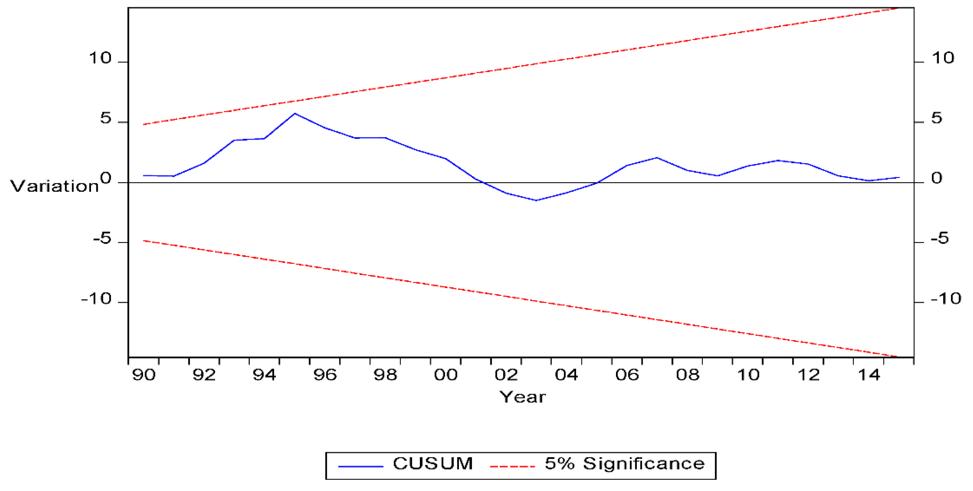
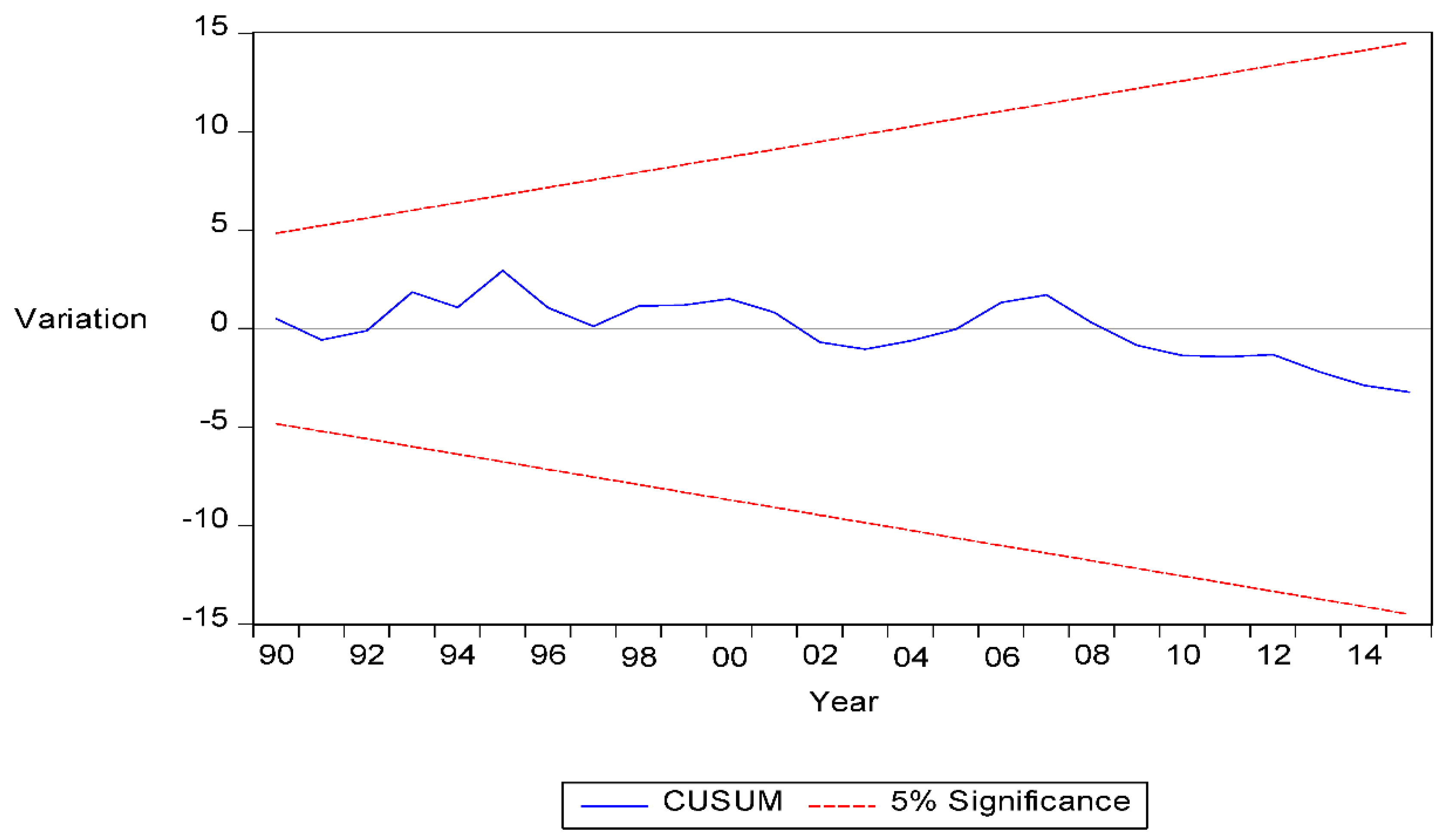
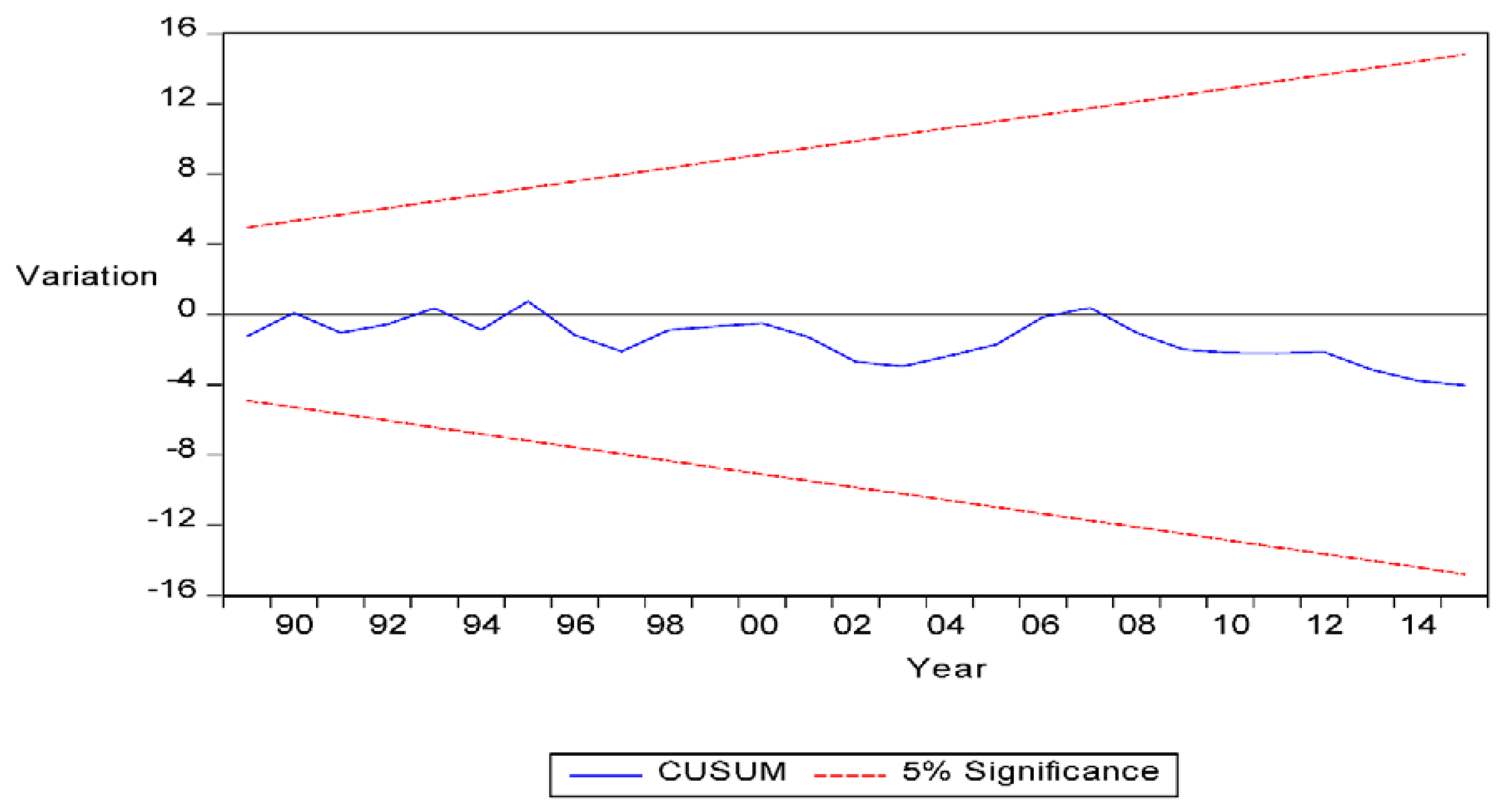
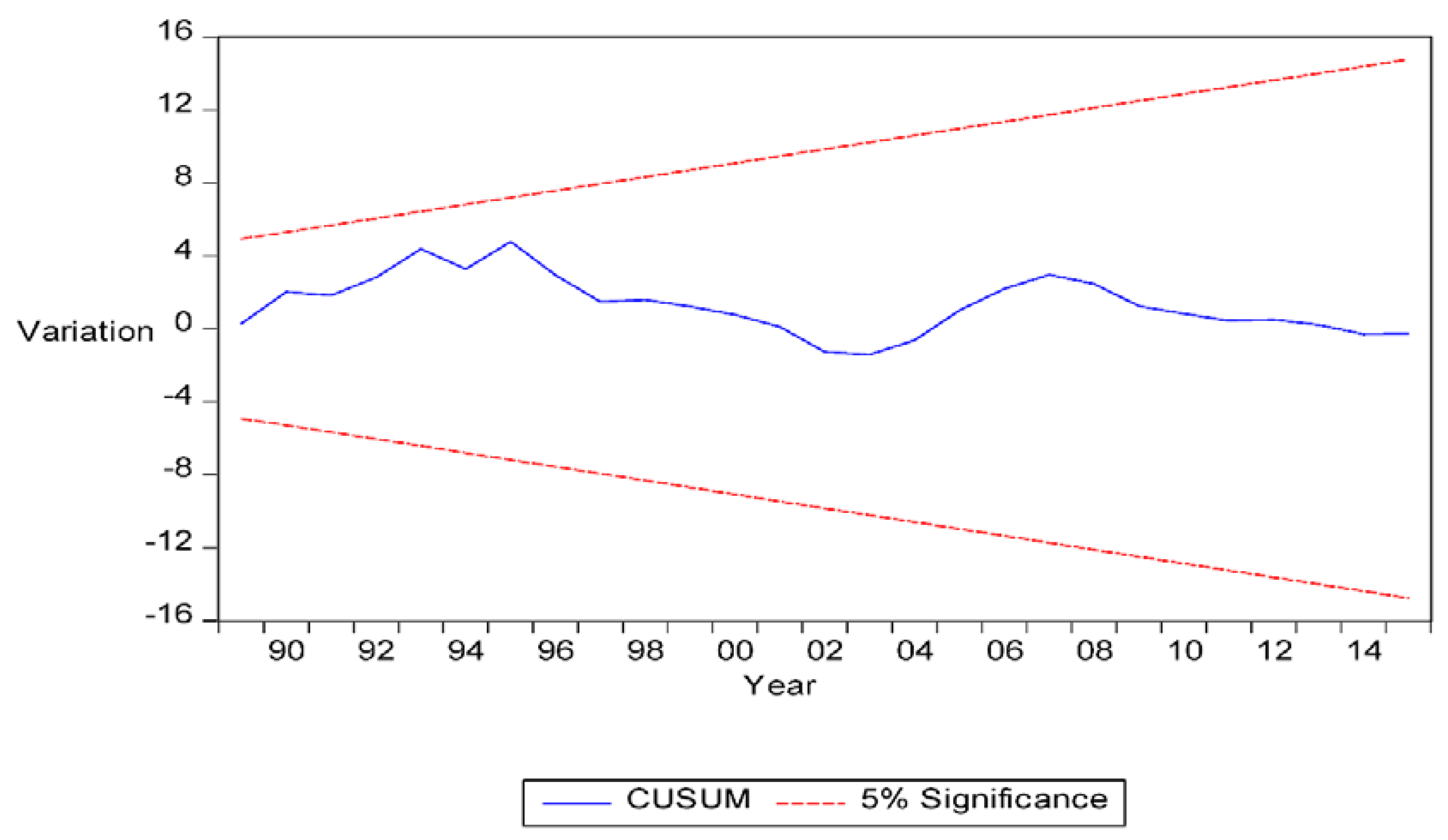
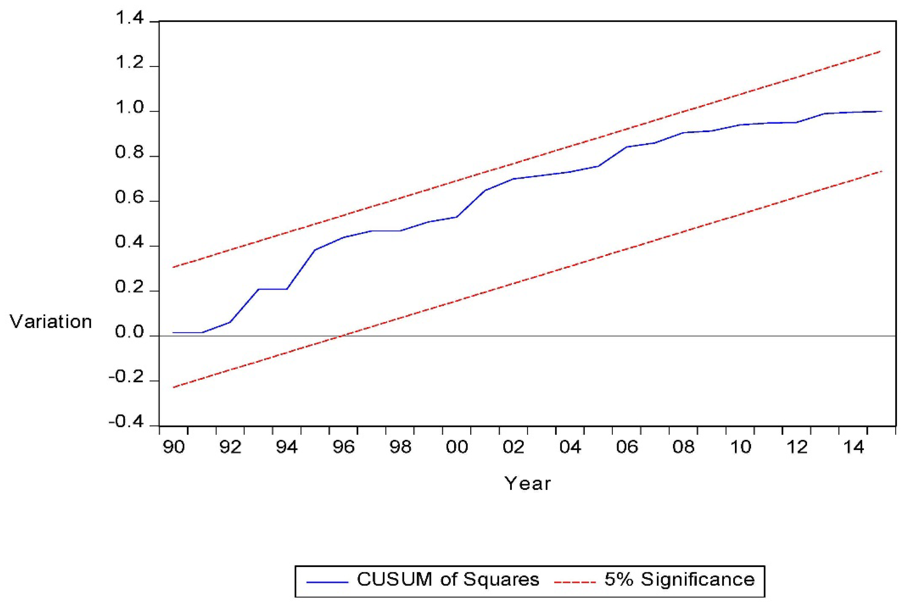
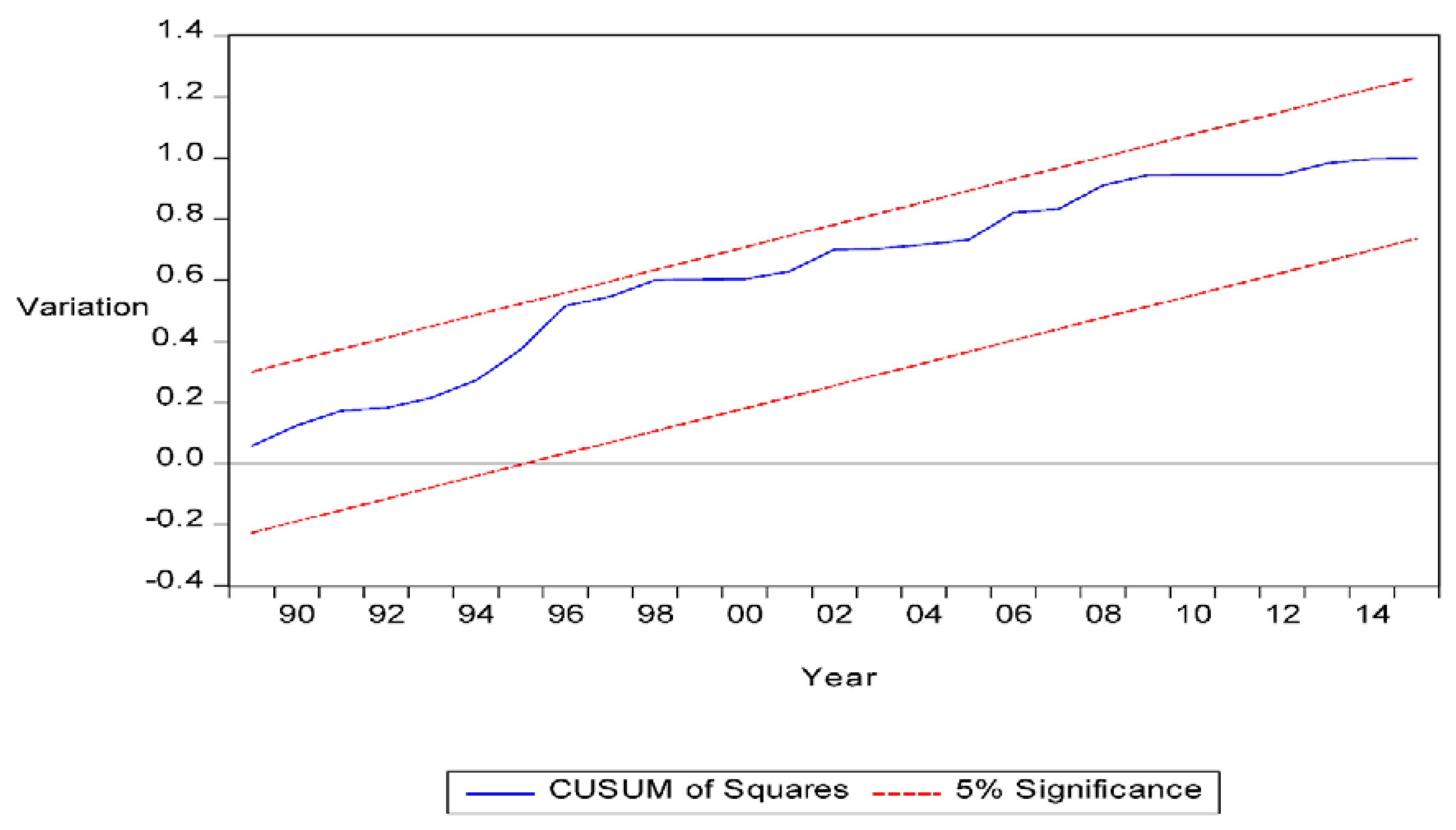
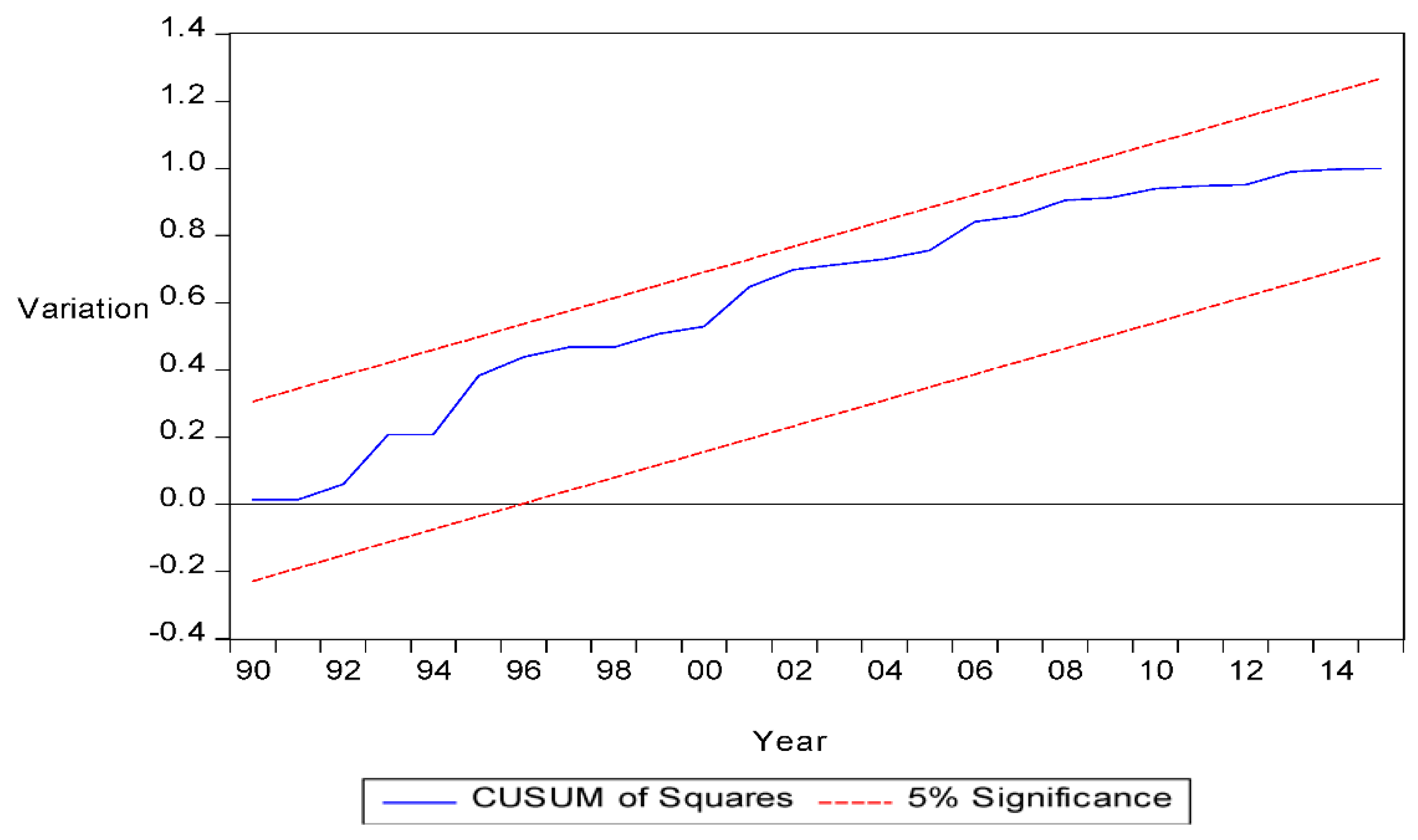
Finally, for ensuring the robustness of the specified models along with both short-run and long-run coefficients, the study used a cumulative sum (CUSUM), and cumulative sum squares (CUSUMSQ) tests proposed by Borensztein et al. (1998). The stability tests based on the Cumulative Sum of Recursive Residuals (CUSUM) and the Cumulative Sum of Squares of Recursive Residuals (CUSUMSQ), reported in Figure 2, Figure 3, Figure 4, Figure 5, Figure 6, Figure 7, Figure 8 and Figure 9 respectively, observe that at the 5% level of significance all the specified models are stable and have test lines that fall within the boundary. It implies model robustness along with the stability of both long run and short run coefficient acceptability over the sample period of 1980–2016.
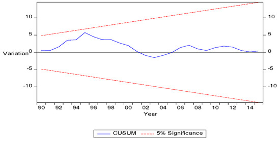
Figure 2.
Plot of CUSUM for MC.
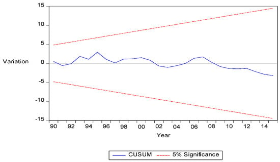
Figure 3.
Plot of CUSUM for TAR.
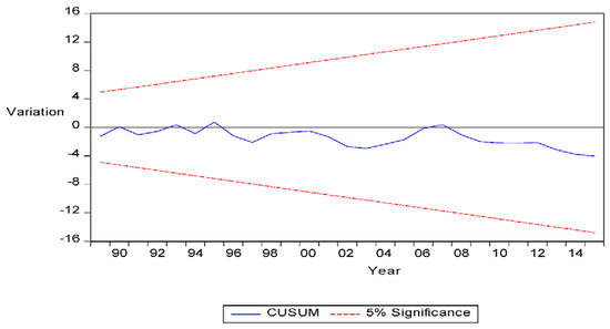
Figure 4.
Plot of CUSUM for TUR.
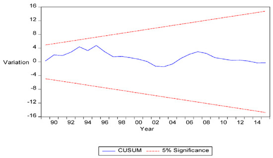
Figure 5.
Plot of CUSUM for M2/M1.
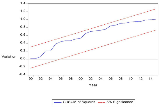
Figure 6.
Plot of CUSUMSQ for MC.
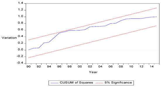
Figure 7.
Plot of CUSUMSQ for TAR.

Figure 8.
Plot of CUSUMSQ for TUR.
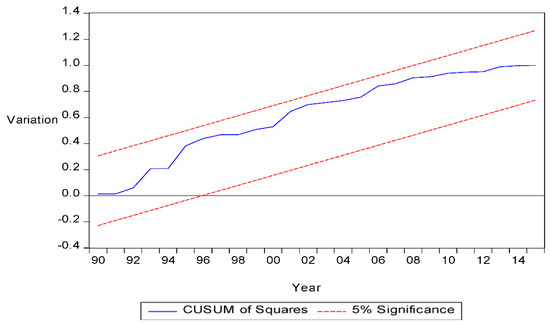
Figure 9.
Plot of CUSUM of Square for F1.
6. Findings and Conclusions
With this study, we examine the relationship between financial innovation, market-based financial development, and economic growth in Bangladesh for the period of 1980–2016. The existing extensive literature shows a number of studies have been conducted to investigate the association between market-based financial developments and economic growth, both in developed and developing countries, however, a few studies had been conducted based on the nexus between the financial development led economic growth of Bangladesh with limited time coverage (see for example, Asghar and Hussain 2014; Duasa 2014; Kabir and Hoque 2007; Masuduzzaman 2014; Sabandi and Noviani 2015; Wadud 2009) and few studies had been conducted that were focused on the market-based financial development led economic growth of Bangladesh (see for example, Mia et al. 2014; Azam et al. 2016; Karim and Chaudhary 2017). By taking into consideration the existing research gap, with this research we intend to explore new insight about market-based financial development along with financial innovation, which use for the first time testing on the Bangladesh economy to capture money supply impact on economic growth using the Broad to Narrow money ratio as a proxy. For empirical investigations, the study employed newly developed ARDL bound testing to capture long-run cointegration between financial innovation, market-based financial development, and economic growth.
ARDL bound testing confirms the existence of long-run cointegration in case of all four tested models. More specifically, the F-statistics of each tested model are greater than the upper bound critical value at the 1% level of significance. These study findings provide conclusive evidence in favor of a long-run association between financial innovation, stock market development, and economic growth. The present existing literature supports it (see for example, Coşkun et al. 2017; Enisan and Olufisayo 2009). However, we observe that some empirical studies reported the nonexistence of cointegration between stock market development and economic growth (see for example, Bundoo 2017; Ahmed and Mmolainyane 2014; Osinubi 2010).
For capturing both long run and short elasticities, the study revealed that financial innovation positively influences economic growth both in the short and long run, which is statistically significant as well. Study findings are in line with Qamruzzaman and Wei (2017); Mwinzi (2014); Bara et al. (2016); Bara and Mudxingiri (2016). Financial innovation in the financial system expands financial activities by introducing new and improved financial institutions, financial assets, and financial services, which eventually accelerate economic activity in the economy. Economic theory explained that financial innovation accelerated financial development with fostering an efficient financial system and accelerating economic movement (Chou and Chin 2011; Beck et al. 2014). On the other hand, proxy variables of stock market development also show a positive influence with statistical significance as well, which is in line with Kajurová and Rozmahel (2016); Caporale et al. (2004); Masoud (2013); Ahmad et al. (2016); Tachiwou (2010); Nyasha and Odhiambo (2016). It is implying that market-based financial developments will lead to sustainable economic growth in the long run by ensuring an efficient financial sector, easy access to financial institutions, the emergence of diversified financial institutions, capital accumulation, and the adequacy of long-term capital. A well performing capital market extends a country’s ability to utilize economic resources more efficiently, rather than having no stock market in the economy (Owusu and Odhiambo 2014; Odhiambo 2010; Ngare et al. 2014).
Furthermore, the study performs the Granger causality test the under error correction model (ECM) and considers empirically tested models for specifying directional causality. Study results revealed bi-directional causality both in the short and long run; these findings are in line with Bara et al. (2016). Financial innovation in the economy brings changes to the financial system by transforming financial services and restructuring financial institutions with an innovative financial proposition. Financial innovation, therefore, is treated as a driver for economic growth (Lumpkin 2010; Sekhar and Gudimetla 2013). On the other hand, stock market development also exhibits bi-directional causality with economic development. This finding is constant with (Ishioro 2013; Silva et al. 2018; Ake and Ognaligui 2010; Antonios 2010; Chizea 2012; Cavenaile et al. 2014). The efficient financial market in the economy can cause economic growth by ensuring optimal mobilization funds, efficient allocation of economic resources, and lowering the cost of capital by expediting capital accumulation processes in the financial system, which in turn thus lead to sustainable economic growth.
With the findings of this study, we bring forth the following two policy recommendations;
- In regards to the financial innovation and economic growth nexus: financial innovation plays a fundamental role in financial sector development. It is because financial innovation expands financial activities in the economy with the emergence of new forms and structures of financial institutions, better financial services through technological advancement, improved financial products, and capital accumulation by encouraging saving in the society, which in turn lead to economic development. Furthermore, an efficient financial sector requires financial innovation, which allows efficient allocation of economic resources in the economy in productive ways. Therefore, the government should make the financial sector more financial innovation-oriented to provide financial services to a large number of households, who can then contribute towards the development process.
- It is inevitable that a well-functioning stock market promotes economic growth, especially in developing countries, like Bangladesh. The efficient stock market allows investors to raise long-term capital easily, which attracts not an only domestic investment but also attracts foreign investors as well. Stock market development, therefore, enhances financial development with productivity in the economy
Author Contributions
The concept and design of this article come from J.W., and thereafter data collection, empirical study review of conceptual development and drafting done by M.Q., and finally critical review and import intellectual content assessment done by J.W. Considering effort by authors in the article, the ration of contribution equally likely.
Funding
The authors do not receive any financial assistant from any agency. All the cost associated of preparing article bear by authors solely.
Conflicts of Interest
The authors, hereby, declaring that no support from any organization for the submitted work; no financial relationships with any organizations that might have an interest in the submitted work; no other relationships or activities that could appear to have influenced the submitted work.
References
- Abdul-Khaliq, Shatha. 2013. The Impact of Stock Market Liquidity on Economic Growth in Jordan. European Journal of Business and Management 5: 154–59. [Google Scholar]
- Adjasi, Charles K. D., and Nicholas B. Biekpe. 2006. Stock Market Development and Economic Growth: The Case of Selected African Countries. Journal Compilation 18: 144–61. [Google Scholar] [CrossRef]
- Adu-Asare Idun, Anthony, and Anthony Q. Q. Aboagye. 2014. Bank competition, financial innovations and economic growth in Ghana. African Journal of Economic and Management Studies 5: 30–51. [Google Scholar] [CrossRef]
- Ahmad, Rubi, Oyebola Fatima Etudaiye-Muhtar, Bolaji Tunde Matemilola, and Amin Noordin Bany-Ariffin. 2016. Financial market development, global financial crisis and economic growth: Evidence from developing nations. Portuguese Economic Journal 15: 199–214. [Google Scholar] [CrossRef]
- Ahmed, Abdullahi D., and Kelesego K. Mmolainyane. 2014. Financial integration, capital market development and economic performance: Empirical evidence from Botswana. Economic Modelling 42: 1–14. [Google Scholar] [CrossRef]
- Aigbokhan, Ben E. 1995. Financial Development and Economic Growth: A Test of Hypothesis on Supply-Leading and Demand Following Finance. With Evidence on Nigeria, The Nigerian Economic and Financial Review 1: 1–10. [Google Scholar]
- Ajide, Folorunsho. 2015. Financial Innovation and Sustainable Development in Selected Countries in West Africa. Innovation in Finance 15: 85–112. [Google Scholar] [CrossRef]
- Ake, Boubakari, and Rachelle Ognaligui. 2010. Financial Stock Market and Economic Growth in Developing Countries: The Case of Douala Stock Exchange in Cameroon. International Journal of Business and Management 5: 82–88. [Google Scholar] [CrossRef]
- Akhavein, Jalal D., W. Scott Frame, and Lawrence J. White. 2001. The diffusion of financial innovations: An examination of the adoption of small business credit scoring by large banking organizations. The Journal of Business 78: 577–96. [Google Scholar] [CrossRef]
- Albentosa, Prats, María Asuncíon, and Beatriz Sandoval. 2016. Stock Market and Economic Growth in Eastern Europe. Kiel: Kiel Institute for the World Economy, pp. 1–35. [Google Scholar]
- Allen, Franklin. 2011. Trends in Financial Innovation and Their Welfare Impact An Overview. Welfare Effects of Financial Innovation 18: 493–514. [Google Scholar] [CrossRef]
- Ansong, Abraham, Edward Marfo-Yiadom, and Emmanuel Ekow-Asmah. 2011. The Effects of Financial Innovation on Financial Savings: Evidence from an Economy in Transition. Journal of African Business 12: 93–113. [Google Scholar] [CrossRef]
- Antonios, Adamopoulos. 2010. Stock Market and Economic Growth: An Empirical Analysis for Germany. Business and Economics Journal 1: 1–12. [Google Scholar]
- Arrau, Patricio. 1991. The Demand for Money in Developing Countries: Assessing the Role of Financial Innovation: World Bank Publications. Washington: World Bank Group. [Google Scholar]
- Asghar, Nabila, and Zakir Hussain. 2014. Financial Development, Trade Openness and Economic Growth in Developing Countries Recent Evidence from Panel Data. Pakistan Economic and Social Review 52: 99–126. [Google Scholar]
- Azam, Muhammad, Muhammad Haseeb, Aznita binti Samsi, and Jimoh Olajide Raji. 2016. Stock Market Development and Economic Growth: Evidences from Asia-4 Countries. International Journal of Economics and Financial Issues 6: 1200–8. [Google Scholar]
- Banerjee, Anindya, Juan J. Dolado, John W. Galbraith, and David Hendry. 1993. Co-Integration, Error Correction, and the Econometric Analysis of Non-Stationary Data. Oxford: Oxford University Press, OUP Catalogue. [Google Scholar]
- Bangladesh Bank. 2017. Annual Report. Dhaka: Bangladesh Bank. [Google Scholar]
- Bangladesh Bureau of Statistics. 2017. National Accounts Statistics—Bangladesh Bureau of Statistics. In Yearly. Bangladesh: Bangladesh Bureau of Statistics, p. 250. [Google Scholar]
- Bara, Alex, and Calvin Mudzingiri. 2016. Financial innovation and economic growth: Evidence from Zimbabwe. Investment Management and Financial Innovations 13: 65–75. [Google Scholar] [CrossRef]
- Bara, Alex, Gift Mugano, and Pierre Le Roux. 2016. Financial Innovation and Economic Growth in the SADC. Economic Research Southern Africa 1: 1–23. [Google Scholar] [CrossRef]
- Bayar, Yilmaz. 2016. Institutional Determinants of Stock Market Development in European Union Transition Economies. The Romanian Economic Journal 19: 211–16. [Google Scholar]
- Beck, Thorsten, Tao Chen, Chen Lin, and Frank M. Song. 2016. Financial innovation: The bright and the dark sides. Journal of Banking & Finance 72: 28–51. [Google Scholar]
- Beck, Thorsten, Lemma Senbet, and Witness Simbanegavi. 2014. Financial inclusion and innovation in Africa: An overview. Journal of African Economies 24: i3–i11. [Google Scholar] [CrossRef]
- Bekeart, Geert, and Campbell R. Harvey. 1997. Capital Market as Engine of Economic Grwoth. The Brown Journal of World Affairs 5: 33–53. [Google Scholar]
- Bekhet, Hussain Ali, Ali Matar, and Tahira Yasmin. 2017. CO2 emissions, energy consumption, economic growth, and financial development in GCC countries: Dynamic simultaneous equation models. Renewable and Sustainable Energy Reviews 70: 117–32. [Google Scholar] [CrossRef]
- Bencivenga, Valerie R., and Bruce D. Smith. 1991. Financial Intermediation and Endogenous Growth. The Review of Economic Studies 58: 195–209. [Google Scholar] [CrossRef]
- Bilyk, Valentyna. 2006. Financial Innovations and the Demand for Money in Ukraine. Master’s thesis, Economics Education and Research Consortium, National University of Kyiv-Mohyla Academy, Kiev, Ukraine. [Google Scholar]
- Błach, Joanna. 2011. Financial Innovations and Their Role in the Modern Financial System—Identification and Systematization of the Problem. Financial Internet Quarterly “e-Finanse” 7: 13–26. [Google Scholar]
- Blair, Margaret M. 2011. Financial Innovation, Leverage, Bubbles and the Distribution of Income. Review of Banking & Financial Law 30: 225–311. [Google Scholar]
- Boot, Arnoud, and Matej Marinc. 2010. Financial innovation: Economic growth versus instability in bank-based versus financial market driven economies. International Journal of Business and Commerce 2: 1–32. [Google Scholar]
- Borensztein, Eduardo, Jose De Gregorio, and Jong-Wha Lee. 1998. How does foreign direct investment affect economic growth? Journal of International Economics 45: 115–35. [Google Scholar] [CrossRef]
- Boubakari, Ake, and Dehuan Jin. 2010. The Role of Stock Market Development in Economic Growth: Evidence from Some Euronext Countries. International Journal of Financial Research 1. [Google Scholar] [CrossRef]
- Bundoo, Sunil K. 2017. Stock market development and integration in SADC (Southern African Development Community). Review of Development Finance 7: 64–72. [Google Scholar] [CrossRef]
- Bwire, Thomas, and Andrew Musiime. 2015. Financial Development—Economic Growth Nexus: Empirical Evidence from Uganda. Journal of Social Science 4: 1–18. [Google Scholar]
- Caporale, Guglielmo Maria, Peter G. A. Howells, and Alaa M. Soliman. 2004. Stock Market Development and Economic Growth: The Causal Linkage. Journal of Economic Development 29: 33–50. [Google Scholar]
- Caporale, Guglielmo Maria, Peter Howells, and Alaa M. Soliman. 2003. Endogenous Growth Models and Stock Market Development: Evidence from Four Countries. Review of Development Economics 9: 166–76. [Google Scholar] [CrossRef]
- Carp, Lenuţa. 2012. Can Stock Market Development Boost Economic Growth? Empirical Evidence from Emerging Markets in Central and Eastern Europe. Procedia Economics and Finance 3: 438–44. [Google Scholar] [CrossRef]
- Cavenaile, Laurent, Christian Gengenbach, and Franz Palm. 2014. Stock Markets, Banks and Long Run Economic Growth: A Panel Cointegration-Based Analysis. De Economist 162: 19–40. [Google Scholar] [CrossRef]
- Chang, Tsangyao, and Steven B. Caudill. 2005. Financial development and economic growth: The case of Taiwan. Applied Economics 37: 1329–35. [Google Scholar] [CrossRef]
- Cheng, Xiaoqiang, and Hans Degryse. 2014. The Impact of Bank and Non-Bank Financial Institutions on Local Economic Growth in China. Journal of Financial Services Research 37: 179–99. [Google Scholar] [CrossRef]
- Chizea, John. 2012. Stock Market Development and Economic Growth in Nigeria: A Time Series Study for the period 1980–2007. Ph.D. thesis, Newcastle Business School, Northumbria University, Newcastle upon Tyne, UK; p. 296. [Google Scholar]
- Chou, Yuan K. 2007. Modelling Financial Innovation and Economic Growth. Jounral of Business and Management 2: 1–36. [Google Scholar]
- Chou, Yuan K., and Martin S. Chin. 2011. Financial Innovations and Endogenous Growth. Journal of Economics and Management 25: 25–40. [Google Scholar]
- Comin, Diego, and Ramana Nanda. 2014. Financial Development and Technology Diffusion. Cambridge: Harvard University, p. 33. [Google Scholar]
- Cooray, Arusha. 2010. Do stock markets lead to economic growth? Journal of Policy Modeling 32: 448–60. [Google Scholar] [CrossRef]
- Coşkun, Yener, Ünal Seven, H. Murat Ertuğrul, and Talat Ulussever. 2017. Capital market and economic growth nexus: Evidence from Turkey. Central Bank Review 17: 19–29. [Google Scholar] [CrossRef]
- Craig, R. Sean, Ina Dettmann-Busch, Eduardo Gomes, Garth Greubel, Klaus Liebig, Keith Lui, Roberto Marino, Daniel Mminele, Ram Prasad Bandi, Srichander Ramaswamy, and et al. 2008. Financial Innovation and Emerging Markets: Opportunities for Growth vs. Risks for Financial Stability. Berlin: InWEnt. [Google Scholar]
- De Gregorio, Jose, and Pablo E. Guidotti. 1995. Financial development and economic growth. World Development 23: 433–48. [Google Scholar] [CrossRef]
- Demetriades, Panicos O., and Khaled A. Hussein. 1996. Does financial development cause economic growth? Time-series evidence from 16 countries. Journal of Development Economics 51: 387–411. [Google Scholar] [CrossRef]
- Demetriades, Panicos O., and Kul B. Luintel. 1996. Financial Development, Economic Growth and Banking Sector Controls: Evidence from India. The Economic Journal 106: 359–74. [Google Scholar] [CrossRef]
- Djoumessi, Emilie Chanceline Kinfack. 2009. Financial Development and Economic Growth: A Comparative Study between Cameroon and South Africa. Master’s thesis, University of South Africa, Pretoria, South Africa; pp. 1–165. [Google Scholar]
- Duasa, Jarita. 2014. Financial Development and Economic Growth: The Experiences of Selected OIC Countries. International Journal of Economics and Management 8: 215–28. [Google Scholar]
- Engle, Robert F., and Clive W. J. Granger. 1987. Cointegration and error correction representation: Estimation and testing. Econometrica 55: 251–76. [Google Scholar] [CrossRef]
- Enisan, Akinlo A., and Akinlo O. Olufisayo. 2009. Stock market development and economic growth: Evidence from seven sub-Sahara African countries. Journal of Economics and Business 61: 162–71. [Google Scholar] [CrossRef]
- Epstein, Stephan R. 1992. Regional fairs, institutional innovation, and economic growth in late medieval Europe 1. The Economic History Review 47: 459–82. [Google Scholar] [CrossRef]
- Gamolya, Andriy. 2006. Stock Market and Economic Growth in Ukraine. Master’s thesis, Economics Education and Research Consortium, National University of Kyiv-Mohyla Academy, Kiev, Ukraine; pp. 1–48. [Google Scholar]
- Geiger, Theodor. 1960. The Stages of Economic Growth: A Non-Communist Manifesto. Edited by Walt Whitman Rostow. New York: Cambridge University Press. [Google Scholar]
- Ghatak, Subrata, and Jalal U. Siddiki. 2001. The use of the ARDL approach in estimating virtual exchange rates in India. Journal of Applied Statistics 28: 573–83. [Google Scholar] [CrossRef]
- Glaeser, Edward L., Rafael La Porta, Florencio Lopez-de-Silanes, and Andrei Shleifer. 2004. Do Institutions Cause Growth? Cambridge: National Bureau of Economic Research. [Google Scholar]
- Gurley, John G., and Edward S. Shaw. 1955. Financial Aspects of Economic Development. American Economic Review 45: 516–37. [Google Scholar]
- Handa, Jagdish, and Shubha Rahman Khan. 2008. Financial development and economic growth: A symbiotic relationship. Applied Financial Economics 18: 1033–49. [Google Scholar] [CrossRef]
- Hellwig, Martin. 1991. Banking, financial intermediation and corporate finance. European Financial Integration, 35–63. [Google Scholar] [CrossRef]
- Ishioro, Bernard O. 2013. Stock Market Development and Economic Growth: Evidence from Zimbabwe. Stock Market 22: 343–60. [Google Scholar]
- Jahfer, Athambawa, and Tohru Inoue. 2014. Stock market development and economic growth in Sri Lanka. International Journal of Business and Emerging Markets 6: 271. [Google Scholar] [CrossRef]
- Jedidia, Khoutem Ben, Thouraya Boujelbène, and Kamel Helali. 2014. Financial development and economic growth: New evidence from Tunisia. Journal of Policy Modeling 36: 883–98. [Google Scholar] [CrossRef]
- Johansen, Søren, and Katarina Juselius. 1990. Maximum Likelihood Estimation and Inference on Cointegration—With Applications to the Demand for Money. Oxford Bulletin of Economics and Statistics 51: 169–210. [Google Scholar] [CrossRef]
- Johansen, Søren. 1991. Estimation and Hypothesis Testing of Cointegration Vectors in Gaussian Vector Autoregressive Models. Econometrica 59: 1551–80. [Google Scholar] [CrossRef]
- Johansen, Søren. 1995. Likelihood-Based Inference in Cointegrated Vector Autoregressive Models. Oxford: Oxford University Press. [Google Scholar]
- Johnson, Simon, and James Kwak. 2012. Is Financial Innovation Good for the Economy? In Innovation Policy and the Economy. Edited by James Lerner and Scott Stern. Chicago: University of Chicago Press, pp. 1–15. [Google Scholar]
- Juhkam, Andres. 2003. Financial Innovation in Estonia. Tallinn: Poliitikauuringute Keskus Praxis. [Google Scholar]
- Kabir, Sarkar Humayun, and Hafiz Al Asad Bin Hoque. 2007. Financial Liberalization, Financial Development and Economic Growth: Evidence from Bangladesh. Savings and Development 4: 431–48. [Google Scholar]
- Kajurová, Veronika, and Petr Rozmahel. 2016. Stock Market Development and Economic Growth: Evidence from the European Union. Acta Universitatis Agriculturae et Silviculturae Mendelianae Brunensis 64: 1927–36. [Google Scholar]
- Karim, Saba, and Ghulam Mujtaba Chaudhary. 2017. Effect of Stock Market Development on Economic Growth of Major South Asian and East Asian Economies: A Comparative Analysis. Journal of Business Studies Quarterly 8: 81–88. [Google Scholar]
- Kassimatis, Konstantinos. 2000. Stock Market Development and Economic Growth in Emerging Economies. Ph.D. thesis, Middlesex University, London, UK; p. 277. [Google Scholar]
- Jedidia, Khoutem Ben, Thouraya Boujelbène, and Kamel Helali. 2014. Financial development and economic growth: New evidence from Tunisia. Journal of Policy Modeling 36: 883–98. [Google Scholar] [CrossRef]
- King, Robert G., and Ross Levine. 1993. Finance and growth: Schumpeter might be right. The Quarterly Journal of Economics 108: 717–37. [Google Scholar] [CrossRef]
- Kothari, Vinod. 2006. Securitization: The Financial Instrument of the Future. Hoboken: John Wiley & Sons. [Google Scholar]
- Kyophilavong, Phouphet, Gazi Salah Uddin, and Muhammad Shahbaz. 2016. The Nexus between Financial Development and Economic Growth in Lao PDR. Global Business Review 17: 303–17. [Google Scholar] [CrossRef]
- Laeven, Luc, Ross Levine, and Stelios Michalopoulos. 2014. Financial Innovation and Endogenous Growth. Stanford: Stanford University. [Google Scholar]
- Levine, Ross. 1997. Financial Development and Economic Growth: Views and Agenda. Journal of Economic Literature 35: 688–726. [Google Scholar]
- Lumpkin, Stephen. 2010. Regulatory issues related to financial innovation. OECD Journal: Financial Market Trends 2: 1–31. [Google Scholar] [CrossRef]
- Magweva, Rabson, and Tafirei Mashamba. 2016. Stock Market Development and Economic Growth: An Empirical Analysis of Zimbabwe (1989–2014). Financial Assets and Investing 7: 20–36. [Google Scholar] [CrossRef]
- Mannah-Blankson, Theresa, and Franklin Belnye. 2004. Financial Innovation and the Demand for Money in Ghana. Accra: Bank of Ghana, pp. 1–23. [Google Scholar]
- Marques, Luís Miguel, José Alberto Fuinhas, and António Cardoso Marques. 2013. Does the stock market cause economic growth? Portuguese evidence of economic regime change. Economic Modelling 32: 316–24. [Google Scholar] [CrossRef]
- Masoud, Najeb M. H. 2013. The Impact of Stock Market Performance upon Economic Growth. International Journal of Economics and Financial Issues 3: 788–98. [Google Scholar]
- Masuduzzaman, Mahedi. 2014. Workers’ Remittance Inflow, Financial Development and Economic Growth: A Study on Bangladesh. International Journal of Economics and Finance 6. [Google Scholar] [CrossRef]
- McGuire, Paul B., and John David Conroy. 2013. Fostering financial innovation for the poor the policy and regulatory environment. In Private Finance for Human Development. Sydney: Foundation for Development Cooperation. [Google Scholar]
- Mia, A. Hannan, Md. Qamruzzaman, and Laila Arjuman Ara. 2014. Stock Market Development and Economic Growth of Bangladesh-A Causal Analysis. Bangladesh Journal of MIS 6: 62–73. [Google Scholar]
- Michalopoulos, Stelios, Luc Laeven, and Ross Levine. 2009. Financial Innovation and Endogenous Growth. Cambridge: National Bureau of Economic Research. [Google Scholar]
- Michalopoulos, Stelios, Luc Laeven, and Ross Levine. 2011. Financial Innovation and Endogenous Growth. Cambridge: National Bureau of Economic Research, pp. 1–33. [Google Scholar]
- Moldovan, Ioana Andrada. 2015. Financial Market’s Contribution to Economic Growth in Romania. Management Dynamics in the Knowledge Economy Journal 3: 447–62. [Google Scholar]
- Morck, Randall, and Masao Nakamura. 1999. Banks and corporate control in Japan. The Journal of Finance 54: 319–39. [Google Scholar] [CrossRef]
- Mwinzi, Dickson Mwangangi. 2014. The Effect of Finanical Innovation on Economic Growth in Kenya. Nairobi: University of Nairobi, p. 54. [Google Scholar]
- Nagayasu, Jun. 2012. Financial innovation and regional money. Applied Economics 44: 4617–29. [Google Scholar] [CrossRef]
- Narayan, Paresh. 2004. Reformulating Critical Values for the Bounds F-Statistics Approach to Cointegration: An Application to the Tourism Demand Model for Fiji. Melbourne: Monash University, pp. 1–40. [Google Scholar]
- Nazir, Mian Sajid, Muhammad Musarat Nawaz, and Usman Javed Gilani. 2010. Relationship between economic growth and stock market development. African Journal of Business Management 4: 3473–79. [Google Scholar]
- Ndako, Umar Bida. 2010. Financial Development, Economic Growth and Stock Market Volatility: Evidence from Nigeria and South Africa. Leicester: University of Leicester. [Google Scholar]
- Ngare, Everlyne, Esman Morekwa Nyamongo, and Roseline N. Misati. 2014. Stock market development and economic growth in Africa. Journal of Economics and Business 74: 24–39. [Google Scholar] [CrossRef]
- Nowbutsing, Baboo M., and M. P. Odit. 2009. Stock Market Development and Economic Growth: The Case of Mauritius. International Business & Economics Research Journal 8: 77–88. [Google Scholar]
- Nsofor, Ebele Sabina. 2016. Impact of Investment on Stock Market Development in Nigeria. International Journal of Financial Economics 5: 1–11. [Google Scholar]
- Nyasha, Sheilla, and Nicholas M. Odhiambo. 2015. Banks, stock market development and economic growth in South Africa: A multivariate causal linkage. Applied Economics Letters 22: 1480–85. [Google Scholar] [CrossRef]
- Nyasha, Sheilla, and Nicholas M. Odhiambo. 2016. Banks, Stock Market Development and Economic Growth in Kenya: An Empirical Investigation. Journal of African Business 18: 1–23. [Google Scholar] [CrossRef]
- Odhiambo, Nicholas M. 2010. Finance-investment-growth nexus in South Africa: An ARDL-bounds testing procedure. Economic Change and Restructuring 43: 205–19. [Google Scholar] [CrossRef]
- Odularu, Gbadebo Olusegun, and Oladapo Adewale Okunrinboye. 2008. Modeling the impact of financial innovation on the demand for money in Nigeria. African Journal of Business Management 3: 39–51. [Google Scholar]
- Ogunmuyiwa, Michael S. 2010. Investor’s Sentiments, Stock Market Liquidity and Economic Growth in Nigeria. Journal of Social Sciences 23: 63–67. [Google Scholar] [CrossRef]
- Orji, Anthony, Jonathan E. Ogbuabor, and Onyinye I. Anthony-Orji. 2015. Financial Liberalization and Economic Growth in Nigeria: An Empirical Evidence. International Journal of Economics and Financial Issues 5: 663–72. [Google Scholar]
- Osinubi, Tokunbo Simbowale. 2010. Does Stock Market Promote Economic Growth In Nigeria? Ibadan: University of Ibadan, pp. 1–29. [Google Scholar]
- Owusu, Erasmus L., and Nicholas M. Odhiambo. 2014. Financial liberalization and economic growth in Nigeria: An ARDL-bounds testing approach. Journal of Economic Policy Reform 17: 164–77. [Google Scholar] [CrossRef]
- Ozcan, Yasar A. 2008. Health Care Benchmarking and Performance Evaluation: An Assessment Using Data Envelopment Analysis (DEA). New York: Springer. [Google Scholar]
- Ozturk, Ilhan, and Ali Acaravci. 2010. CO2 emissions, energy consumption and economic growth in Turkey. Renewable and Sustainable Energy Reviews 14: 3220–25. [Google Scholar] [CrossRef]
- Pagan, Adrian Rodney, and Anthony David Hall. 1983. Diagnostic tests as residual analysis. Econometric Reviews 2: 159–218. [Google Scholar] [CrossRef]
- Pahlavani, Mosayeb, Ed Wilson, and Andrew Charles Worthington. 2005. Trade-GDP nexus in Iran: An application of the autoregressive distributed lag (ARDL) model. Wollongong, New South Wales, Australia: Faculty of Commerce Papers, University of Wollongong. [Google Scholar]
- Perron, Pierre. 1997. Further evidence on breaking trend functions in macroeconomic variables. Journal of Econometrics 80: 355–85. [Google Scholar] [CrossRef]
- Pesaran, H. Hashem, and Yongcheol Shin. 1998. Generalized impulse response analysis in linear multivariate models. Economics Letters 58: 17–29. [Google Scholar] [CrossRef]
- Pesaran, M. Hashem, Yongcheol Shin, and Richard J. Smith. 2001. Bounds testing approaches to the analysis of level relationships. Journal of Applied Econometrics 16: 289–326. [Google Scholar] [CrossRef]
- Petros, Jecheche. 2012. The effect of the stock exchange on economic growth: A case of the Zimbabwe stock exchange. Research in Business and Economics Journal 6: 1. [Google Scholar]
- Phillips, Peter C. B., and Pierre Perron. 1988. Testing for a unit root in time series regression. Biometrika 75: 335–46. [Google Scholar] [CrossRef]
- Pohoaţă, Ion, Delia Elena Diaconaşu, and Oana Ramona Socoliuc. 2016. Economic Dynamics—Stock Market Evolution: A Relation Committed To Dysfunctionality in Romania and Croatia. Ecoforum 5: 332–37. [Google Scholar]
- Pradhan, Rudra P., Mak B. Arvin, and S. Bahmani. 2015. Causal nexus between economic growth, inflation, and stock market development: The case of OECD countries. Global Finance Journal 27: 98–111. [Google Scholar] [CrossRef]
- Pradhan, Rudra P., Mak B. Arvin, John H. Hall, and Sahar Bahmani. 2014a. Causal nexus between economic growth, banking sector development, stock market development, and other macroeconomic variables: The case of ASEAN countries. Review of Financial Economics 23: 155–73. [Google Scholar] [CrossRef]
- Pradhan, Rudra P., Sasikanta Tripathy, Shashikant Pandey, and Samadhan K. Bele. 2014b. Banking sector development and economic growth in ARF countries: The role of stock markets. Macroeconomics and Finance in Emerging Market Economies 7: 208–29. [Google Scholar] [CrossRef]
- Prats, María Asuncíon, and Beatriz Sandoval. 2016. Stock market and economic growth in Eastern Europe. Economics Discussion Papers, Kiel, Germany: Kiel Institute for the World Economy (IfW). [Google Scholar]
- Qamruzzaman, Md., and Jianguo Wei. 2017. Financial innovation and economic growth in Bangladesh. Financial Innovation 3: 19. [Google Scholar] [CrossRef]
- Ram, Rati. 1999. Financial development and economic growth: Additional evidence. Journal of Development Studies 35: 164–74. [Google Scholar] [CrossRef]
- Hasan, Rezwanul, and Suborna Barua. 2015. Financial Development and Economic Growth: Evidence from a Panel Study on South Asian Countries. Asian Economic and Financial Review 5: 1159–73. [Google Scholar]
- Saad, Wadad. 2014. Financial Development and Economic Growth: Evidence from Lebanon. International Journal of Economics and Finance 6. [Google Scholar] [CrossRef]
- Sabandi, Muhammad, and Leny Noviani. 2015. The Effects of Trade Liberalization, Financial Development and Economic Crisis on Economic Growth in Indonesia. Journal of Economics and Sustainable Development 6: 120–28. [Google Scholar]
- Huntington, Samuel. P. 1993. The Third Wave: Democratization in the Late Twentieth Century. Norman: University of Oklahoma Press. [Google Scholar]
- Saqib, Najia. 2013. Impact of Development and Efficiency of Financial Sector on Economic Growth: Empirical Evidence from Developing Countries. Journal of Knowledge Management, Economics and Information Technology 3: 1–15. [Google Scholar]
- Saqib, Najia. 2015. Review of Literature on Finance-Growth Nexus. Journal of Applied Finance & Banking 5: 175–95. [Google Scholar]
- Schrieder, Gertrud, and Franz Heidhues. 1995. Reaching the Poor through Financial Innovations. Quarterly Journal of International Agriculture 2: 132–48. [Google Scholar]
- Schumpeter, Joseph. 1911. The Theory of Economic Development. Cambridge: Harvard University Press. [Google Scholar]
- Sekhar, Satya, and V. Gudimetla. 2013. Theorems and Theories of Financial Innovation: Models and Mechanism Perspective. Financial and Quantitative Analysis 1: 26–29. [Google Scholar] [CrossRef]
- Seven, Ünal, and Hakan Yetkiner. 2016. Financial intermediation and economic growth: Does income matter? Economic Systems 40: 39–58. [Google Scholar] [CrossRef]
- Shahbaz, Muhammad, Ijaz Ur Rehman, and Ahmed Taneem Muzaffar. 2015. Re-Visiting Financial Development and Economic Growth Nexus: The Role of Capitalization in Bangladesh. South African Journal of Economics 83: 452–71. [Google Scholar] [CrossRef]
- Shaughnessy, Haydn. 2015. Innovation in Financial Services: The Elastic Innovation Index Report. La Hulpe: Innotribe. 21p. [Google Scholar]
- Shittu, Ayodele Ibrahim. 2012. Financial Intermediation and Economic Growth in Nigeria. British Journal of Arts and Social Sciences 4: 164–79. [Google Scholar]
- Silva, N. K. L., P. R. M. R. Perera, and N. L. C. Silva. 2018. Relationship between Stock Market Performance & Economic Growth: Empirical Evidence from Sri Lanka. Journal for Accounting Researchers and Educators 1: 1. [Google Scholar]
- Silve, Florent, and Alexander Plekhanov. 2014. Institutions, Innovation and Growth: Cross-Country Evidence. London: European Bank for Reconstruction and Development, p. 28. [Google Scholar]
- Simiyu, Robert Silikhe, Paul Nyatha Ndiang’ui, and Celestine Chege Ngugi. 2014. Effect of Financial Innovations and Operationalization on Market Size in Commercial Banks: A Case Study of Equity Bank, Eldoret Branch. International Journal of Business and Social Science 85: 227–50. [Google Scholar]
- Smaoui, Houcem, and Salem Nechi. 2017. Does sukuk market development spur economic growth? Research in International Business and Finance 41: 136–47. [Google Scholar] [CrossRef]
- Soyode, Afolabi. 1990. The role of capital market in economic development. Security Market Journal in Nigeria 6: 223–254. [Google Scholar]
- Tachiwou, Aboudou Maman. 2010. Stock Market Development and Economic Growth: The Case of West African Monetary Union. Nternational Journal of Economics and Finance 2: 97–103. [Google Scholar] [CrossRef]
- Van Nieuwerburgh, Stijn, Frans Buelens, and Ludo Cuyvers. 2006. Stock market development and economic growth in Belgium. Explorations in Economic History 43: 13–38. [Google Scholar] [CrossRef]
- Wachter, Jessica A. 2006. Comment on: “Can financial innovation help to explain the reduced volatility of economic activity?”. Journal of Monetary Economics 53: 151–54. [Google Scholar] [CrossRef]
- Wadud, Md. Abdul. 2009. Financial development and economic growth: A cointegration and errorcorrection modeling approach for south Asian countries. Economics Bulletin 29: 1670–77. [Google Scholar]
- Weinstein, David E., and Yishay Yafeh. 1998. On the costs of a bank-centered financial system: Evidence from the changing main bank relations in Japan. The Journal of Finance 53: 635–72. [Google Scholar] [CrossRef]
- Wong, Anson, and Xianbo Zhou. 2011. Development of Financial Market and Economic Growth: Review of Hong Kong, China, Japan, The United States and The United Kingdom. International Journal of Economics and Finance 3: 111–15. [Google Scholar] [CrossRef]
- World Bank. 2017. World Development Indicators. Available online: http://data.worldbank.org/data-catalog/world-development-indicators (accessed on 1 June 2017).
- World Economic Outlook. 2017. World Economic Outlook (WEO) Data. IMF. Available online: https://www.imf.org/external/pubs/ft/weo/2017/02/weodata/index.aspx (accessed on 1 June 2017).
- Zivot, Eric, and Donald W. K. Andrews. 2002. Further evidence on the great crash, the oil-price shock, and the unit-root hypothesis. Journal of Business & Economic Statistics 20: 25–44. [Google Scholar]
© 2018 by the authors. Licensee MDPI, Basel, Switzerland. This article is an open access article distributed under the terms and conditions of the Creative Commons Attribution (CC BY) license (http://creativecommons.org/licenses/by/4.0/).

