Modeling and Predictability of Exchange Rate Changes by the Extended Relative Nelson–Siegel Class of Models

Abstract
:1. Introduction
Related Literature
2. Model
2.1. The Present Value Model
2.2. The Relative Nelson–Siegel Model
2.2.1. The Original Chen and Tsang (2013) Model
2.2.2. Extended Model 1: Four-Factor Model Based on Svensson (1994)
2.2.3. Extended Model 2: Five-Factor Model Based on De Rezende and Ferreira (2013)
3. Estimation of Decaying Parameter and Relative Factors
4. Modeling and Estimation Results
4.1. Uncovered Interest Rate Parity
4.2. In-Sample-Fit Forecast Estimation
- (1)
- We created error terms that affected one-month-ahead exchange rate movement. To do so, we first regressed one-month exchange rate changes on a constant term and kept the standard error of the regression as . Then, a vector of error terms of the mean zero, and the volatility was generated from the standard normal random variable.
- (2)
- We created error terms (m = 3, 6, 12) that generated m-month-ahead exchange rate movements at given time t. As Chen and Tsang (2013) mention, there was a problem with inference bias when we analyzed the longer-horizon predictability using the overlapping data. If we used 3-, 6-, and 12-month exchange rate changes, the variables overlap across observations, and the error term in Equations (11)–(13) became a moving average process of order . To solve this issue of inference bias, we constructed an error term as a moving average, i.e., . The generated data were the same length as the actual data.
- (3)
- We estimated the mean return of m-month-ahead exchange rate movement. To do so, we regressed the actual -month (m = 3, 6, 12) exchange rate changes on a constant and kept the constant term , respectively.
- (4)
- We created the artificial exchange rate changes to be . Then, we estimated the CH-UIRP, SV-UIRP, and FF-UIRP regression model (Equations (11)–(13)) using the artificial exchange rate changes as the dependent variable in rolling regressions for a five-year window.
4.3. Out-of-Sample Prediction
4.4. Clark and West Test
5. Conclusions
Acknowledgments
Conflicts of Interest
References
- Chen, Yu-Chin, and Kwok Ping Tsang. 2013. What does the yield curve tell us about exchange rate predictability? Review of Economics and Statistics 95: 185–205. [Google Scholar] [CrossRef]
- Christensen, Jens H. E., Francis X. Diebold, and Glenn D. Rudebusch. 2009. An arbitrage-free generalized Nelson–Siegel term structure model. Econometrics Journal 12: C33–C64. [Google Scholar] [CrossRef]
- Christensen, Jens H. E., Francis X. Diebold, and Glenn D. Rudebusch. 2011. The affine arbitrage-free class of Nelson-Siegel term structure models. Journal of Econometrics 164: 4–20. [Google Scholar] [CrossRef]
- Clark, Todd E., and Kenneth D. West. 2006. Using out-of-sample mean squared prediction errors to test the martingale difference hypothesis. Journal of Econometrics 135: 155–86. [Google Scholar] [CrossRef]
- Cox, John, Jonathan E. Ingersoll Jr., and Stephen A. Ross. 1985. A theory of the term structure of interest rates. Econometrica 53: 385–407. [Google Scholar] [CrossRef]
- De Rezende, Rafael B., and Mauro S. Ferreira. 2013. Modeling and forecasting the yield curve by an extended Nelson-Siegel class of models; a quantile autoregression approach. Journal of Forecasting 32: 111–23. [Google Scholar] [CrossRef]
- Diebold, Francis X., and Canlin Li. 2006. Forecasting the term structure of government bond yields. Journal of Econometrics 130: 337–64. [Google Scholar] [CrossRef]
- Diebold, Francis X., and Robert S. Mariano. 1995. Comparing predictive accuracy. Journal of Business and Economic Statistics 13: 134–44. [Google Scholar]
- Duffie, Darrell, and Rui Kan. 1996. A yield factor model of interest rates. Mathematical Finance 6: 379–406. [Google Scholar] [CrossRef]
- Engel, Charles, and Kenneth D. West. 2006. Taylor rules and the Deutschmark-Dollar real exchange rate. Journal of Money, Credit, and Banking 38: 1175–94. [Google Scholar] [CrossRef]
- Engel, Charles, Nelson C. Mark, and Kenneth D. West. 2007. Exchange rate models are not as bad as you think. NBER Macroeconomics Annual 22: 381–441. [Google Scholar] [CrossRef]
- Estrella, Arturo, and Gikas A. Hardouvelis. 1991. The yield curve as a predictor of real economic activity. Journal of Finance 46: 555–76. [Google Scholar] [CrossRef]
- Estrella, Arturo, and Frederic S. Mishkin. 1998. Predicting U.S. recessions: Financial variables as leading indicators. Review of Economics and Statistics 1: 45–61. [Google Scholar] [CrossRef]
- Frankel, Jeffrey A. 1979. On the mark: a theory of floating exchange rates based on real interest differentials. American Economic Review 69: 610–23. [Google Scholar]
- Litterman, Robert, and Jose Scheinkman. 1991. Common factors affecting bond returns. Journal of Fixed Income 1: 54–61. [Google Scholar] [CrossRef]
- Mark, Nelson C. 1995. Exchange rates and fundamentals: evidence on long-horizon predictability. American Economic Review 85: 201–18. [Google Scholar]
- Molodtsova, Tanya, Alex Nikolsko-Rzhevskyy, and David H. Papell. 2008. Taylor rules with real-time data: A tale of two countries and one exchange rate. Journal of Monetary Economics 55: 63–79. [Google Scholar] [CrossRef]
- Molodtsova, Tanya, and David H. Papell. 2009. Out of-sample exchange rate predictability with Taylor rule fundamentals. Journal of International Economics 77: 167–80. [Google Scholar] [CrossRef]
- Moon, Roger, Antonio Rubia, and Rossen Valkanov. 2004. Long-Horizon Regressions when the Predictor is Slowing Varying. San Diego Working Paper. Oakland, CA, USA: University of California. [Google Scholar]
- Mussa, Michael. 1976. The exchange rate, the balance of payments and monetary and fiscal policy under a regime of controlled floating. Scandinavian Journal of Economics 78: 229–48. [Google Scholar] [CrossRef]
- Nelson, Charles R., and Andrew F. Siegel. 1987. Parsimonious modeling of yield curves. Journal of Business 60: 473–89. [Google Scholar] [CrossRef]
- Rossi, Barbara. 2013. Exchange rate predictability. Journal of Economic Literature 51: 1063–119. [Google Scholar] [CrossRef]
- Svensson, Lars E. 1994. Estimating and Interpreting Forward Interest Rates: Sweden 1992–1994. NBER Working Paper Series No.4871; Cambridge, CA, USA: National Bureau of Economic Research. [Google Scholar]
- Valkanov, Rossen. 2003. Long-horizon regressions: theoretical results and applications. Journal of Financial Economics 68: 201–32. [Google Scholar] [CrossRef]
- Vasicek, Oldrich. 1977. An equilibrium characterization of the term structure. Journal of Financial Economics 5: 177–88. [Google Scholar] [CrossRef]
- West, Kenneth D. 1996. Asymptotic inference about predictive ability. Econometrica 64: 1067–84. [Google Scholar] [CrossRef]
| 1 | Christensen et al. (2009, 2011) impose arbitrage-free pricing theory on the dynamic Nelson–Siegel model. |
| 2 | |
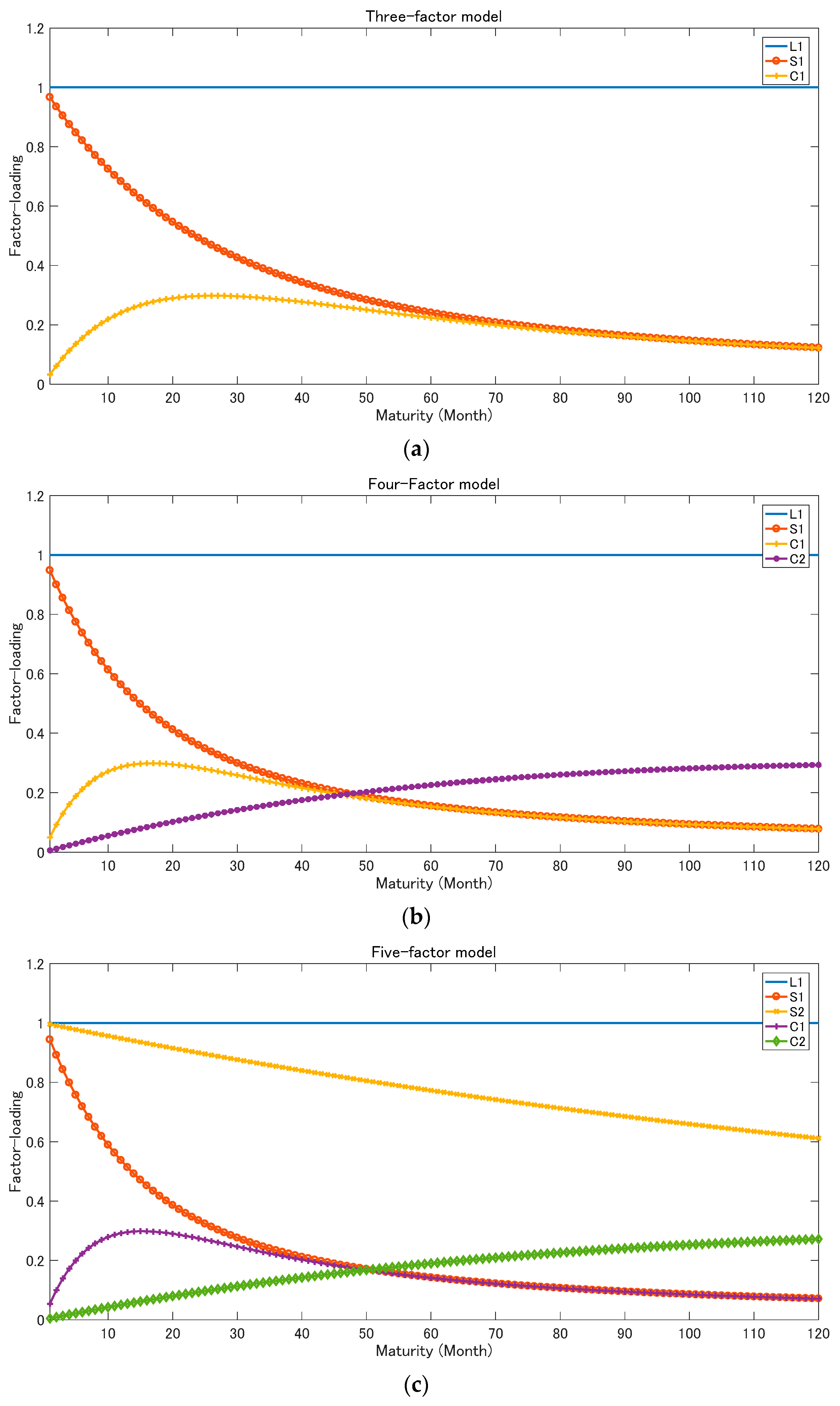
| 3 | Litterman and Scheinkman (1991) show that the dynamics of the yield curve are explained well by the first three principal components. Moreover, the first, second, and third components are specified as level, slope, and curvature of the yield curve. |
| 4 | We regard the prevailing interest rates published by the Ministry of Finance as the per yields, and estimate the Japanese zero coupon yield from those of the data by using MATLAB financial toolbox and financial instrument toolbox. |
| 5 | These models are the restricted model of . |
| 6 | Following Chen and Tsang (2013), Valkanov (2003), and Moon et al. (2004), we use the rescaled statistic value . |
| 7 |

| Three-Factor(CH) | Four-Factor(SV) | Five-Factor(FF) | |
|---|---|---|---|
| 0.068 | 0.107 | 0.117 | |
| 0.012 | 0.009 |
| Mean | Volatility | 1-Lag Coefficient | 12-Lag Coefficient | |
|---|---|---|---|---|
| 3-factor model | ||||
| 0.028 | 0.008 | 0.928 | 0.580 | |
| −0.010 | 0.019 | 0.977 | 0.625 | |
| 0.006 | 0.006 | 0.962 | 0.728 | |
| 4-factor model | ||||
| 0.017 | 0.048 | 0.936 | 0.589 | |
| −0.0002 | 0.035 | 0.895 | 0.357 | |
| 0.016 | 0.030 | 0.856 | 0.184 | |
| 0.033 | 0.127 | 0.929 | 0.522 | |
| 5-factor model | ||||
| 0.015 | 0.107 | 0.933 | 0.766 | |
| −0.005 | 0.030 | 0.916 | 0.610 | |
| 0.006 | 0.071 | 0.909 | 0.702 | |
| 0.012 | 0.023 | 0.818 | 0.237 | |
| 0.031 | 0.215 | 0.938 | 0.753 |
| 3-Month-Ahead | |||||
| CH | −0.962 | 0.646 | ― | −0.169 | ― |
| -value | −1.426 | 1.454 | ― | −0.699 | ― |
| SV | −1.813 | 1.137 | ― | −0.677 | −0.952 |
| -value | −2.598 *** | 2.229 ** | ― | −2.483 ** | −3.499 *** |
| FF | −1.866 | 1.185 | −0.259 | −0.683 | −0.989 |
| -value | −2.603 *** | 2.240 ** | −0.647 | −2.107 ** | −3.435 *** |
| 6-Month-Ahead | |||||
| CH | −1.590 | 1.516 | ― | −0.460 | ― |
| -value | −1.176 | 1.706 * | ― | −0.951 | ― |
| SV | −2.739 | 2.251 | ― | −0.995 | −1.569 |
| -value | −1.951 * | 2.188 ** | ― | −1.812 * | −2.866 *** |
| FF | −2.873 | 2.297 | −0.293 | −0.908 | 0.116 |
| -value | −1.992 ** | 2.160 ** | −0.367 | −1.392 | 2.527 ** |
| 12-Month-Ahead | |||||
| CH | −2.715 | 1.774 | ― | −0.261 | ― |
| -value | −1.059 | 1.054 | ― | −0.286 | ― |
| SV | −3.882 | 2.408 | ― | −0.729 | −2.134 |
| -value | −1.432 | 1.212 | ― | −0.687 | −2.018 ** |
| FF | −4.083 | 2.407 | −0.568 | −0.580 | −2.21 |
| -value | −1.466 | 1.172 | −0.367 | −0.459 | −1.980 ** |
| 3-month | 0.000 | 0.000 | 0.000 |
| 6-month | 0.000 | 0.000 | 0.000 |
| 12-month | 0.000 | 0.000 | 0.000 |
| RW | CH | SV | FF | |
|---|---|---|---|---|
| 3-month | 0.1643 | 0.1073 | 0.1076 | 0.1079 |
| 6-month | 0.3647 | 0.1886 | 0.1886 | 0.1882 |
| 12-month | 0.5941 | 0.1668 | 0.1667 | 0.1659 |
| 3-Month | CH | SV | FF |
|---|---|---|---|
| RW | 4.94 | 3.1 | 3.28 |
| -value | 0.000 | 0.001 | 0.001 |
| CH | ― | −1.29 | −1.3 |
| -value | ― | 0.901 | 0.903 |
| SV | ― | ― | 1.46 |
| -value | ― | ― | 0.072 |
| 6-month | |||
| RW | 11.78 | 12.19 | 13.63 |
| -value | 0.000 | 0.000 | 0.000 |
| CH | ― | −2.79 | −1.91 |
| -value | ― | 0.997 | 0.971 |
| SV | ― | ― | 2.71 |
| -value | ― | ― | 0.003 |
| 12-month | |||
| RW | 2.73 | 2.63 | 2.64 |
| -value | 0.003 | 0.004 | 0.004 |
| CH | ― | -2.12 | -1.42 |
| -value | ― | 0.983 | 0.922 |
| SV | ― | ― | 2.91 |
| -value | ― | ― | 0.002 |
© 2018 by the author. Licensee MDPI, Basel, Switzerland. This article is an open access article distributed under the terms and conditions of the Creative Commons Attribution (CC BY) license (http://creativecommons.org/licenses/by/4.0/).
Share and Cite
Ishii, H. Modeling and Predictability of Exchange Rate Changes by the Extended Relative Nelson–Siegel Class of Models. Int. J. Financial Stud. 2018, 6, 68. https://doi.org/10.3390/ijfs6030068
Ishii H. Modeling and Predictability of Exchange Rate Changes by the Extended Relative Nelson–Siegel Class of Models. International Journal of Financial Studies. 2018; 6(3):68. https://doi.org/10.3390/ijfs6030068
Chicago/Turabian StyleIshii, Hokuto. 2018. "Modeling and Predictability of Exchange Rate Changes by the Extended Relative Nelson–Siegel Class of Models" International Journal of Financial Studies 6, no. 3: 68. https://doi.org/10.3390/ijfs6030068
APA StyleIshii, H. (2018). Modeling and Predictability of Exchange Rate Changes by the Extended Relative Nelson–Siegel Class of Models. International Journal of Financial Studies, 6(3), 68. https://doi.org/10.3390/ijfs6030068