Article

Macroeconomic Stability in a Model with Bond Transaction Services

by
Massimiliano Marzo
1,* and
Paolo Zagaglia
2,*
1
Department of Management, Università di Bologna, Via Capo di Lucca 34, 40126 Bologna, Italy
2
Rimini Centre for Economic Analysis and School of Political Science (Ravenna Campus), Università di Bologna, Via degli Ariani 1, 48121 Ravenna, Italy
*
Authors to whom correspondence should be addressed.
Int. J. Financial Stud. 2018, 6(1), 23; https://doi.org/10.3390/ijfs6010023
Submission received: 31 December 2017 / Revised: 11 February 2018 / Accepted: 12 February 2018 / Published: 22 February 2018

Abstract

:
Cochrane (2014) shows that high-powered money balances and short-term government bonds can be considered as perfect substitutes for the U.S economy during the past twenty years. We build on this claim and consider a variant of the standard cashless new-Keynesian model with two types of government bonds, which can be thought of as short- and long-term bonds. The first one has a macroeconomic role in the sense that it provides transaction services in addition to generating a yield. The other type of government bond pays only an interest rate. Consistent with previous findings, the Taylor principle is not a panacea for equilibrium determinacy in a model without money. When the government bond market matters beyond the need for fiscal solvency, monetary policy rules do not need to comply with the Taylor principle for unique equilibria to exist.

1. Introduction

On 10 February 2010, Fed Chairman Ben S. Bernanke testified before the U.S. House of Representatives Committee on Financial Services with a statement titled “Federal Reserve’s exit strategy”. His speech included the following remarks:
Most importantly, in October 2008 the Congress gave the Federal Reserve statutory authority to pay interest on banks’ holdings of reserve balances. By increasing the interest rate on reserves, the Federal Reserve will be able to put significant upward pressure on all short-term interest rates, as banks will not supply short-term funds to the money markets at rates significantly below what they can earn by holding reserves at the Federal Reserve Banks.
Interestingly, in Bernanke’s view, the experience from the payment of interest rates on banks’ reserves could provide useful guidance for amending the operational framework for the Fed monetary policy:1
The authority to pay interest on reserves is likely to be an important component of the future operating framework for monetary policy. For example, one approach is for the Federal Reserve to bracket its target for the federal funds rate with the discount rate above and the interest rate on excess reserves below.
This type of monetary policy action has gone hand in hand with large-scale asset purchases by the Fed. On 1 December 2008, Bernanke (2008) announced publicly that the Fed “could purchase longer-term Treasury securities (…) in substantial quantities”. By 18 March 2009, the Fed held 300 billion USD of long-term Treasury securities. Hence, a wide array of different policy tools have been put in place since the outbreak of the financial crisis in the U.S. Based on the idea that macroeconomic recovery runs through the ability of the Fed to steer financial markets towards a desired reaction path, many commentators and policy analysts have dwelled on the short-term effects of the Fed decisions (e.g., see Gagnon et al. 2010; Woodford 2012).
One of the consequences of the Fed actions is that high-powered money balances and short-term government bonds have become perfect substitutes for banks. In other words, banks’ reserve balances and short-term U.S. Treasuries pay a similar interest rate. In the experience of ultra-loose liquidity supply by the FED, reserve requirements are far from binding. In terms of macroeconomic outlook, Cochrane (2014) stresses that the U.S. inflation rate has been stable during the past decade, and that there have been small variations in policy and short-term rates. But what are the implications of this macroeconomic landscape for the ability of monetary policy to lead the economy towards a cyclical path of stability? Does that ability that depend only on the decisions by the central bank in a world where the government bond market plays a well-acknowledged role for achieving the objective of macroeconomic stability? These policy-relevant questions are the focus of our paper.
The point of departure of our analysis concerns the interpretation of two facts that have not been fully discussed in the literature yet, and that are centred around the role of government bonds. In a world where short-term bonds can be considered as perfect substitutes for high-powered money, it becomes clear that short-term bonds have an economic property that long-term bonds do not have. This means that the economic differences between short- and long-term bonds are not only about the maturity structure, i.e., about exogenous characteristics.2
The second key to understanding the implications of the perfect substitutability between banks’ reserves and short-term government securities arises from the role of money as a medium of exchange in the provision of ‘transaction services’ that ‘facilitate’ purchases in consumption goods markets.3 In particular, if money and short-term bonds are perfect substitutes, then these bonds can be expected to deliver transaction services in a broad economic sense.
Obviously this discussion is not meant to imply that anyone can go to the grocery and buy, say, apples by posting bonds as a payment instrument or as a guarantee. Inasmuch as economic agents are satiated with cash in modern economies, the macroeconomic role of government bonds is pervasive in enabling the capability of financial markets to finance every day’s economic activities. They are used to perform functions that indirectly facilitate transactions in the real markets, and that contribute to the smooth functioning of final-goods markets. For instance, Aggarwal et al. (2017) suggests that the European government bond lending market allows borrowers to access safe assets and, as such, is an integral part of the short-term funding market.
Our modelling approach for riskless assets as a function of transaction costs has already been considered in the literature. For instance, Vayanos and Vila (1999) study a continuous-time economy with overlapping generations of agents with two assets. One of these carries a transaction cost, while the other is ‘liquid’ in a microeconomic sense. Vayanos and Vila (1999) show that, in equilibrium, the price difference depends on the relative asset supply.
Based on these considerations, we study the ability of a central bank to pin down determine macroeconomic equilibria in a standard New Keynesian model with two types of bonds.4 The first type provides transaction services that are accounted for in the purchase of consumption goods. It pays the policy rate as a yield. The other bond performs the usual function of store of value, and pays an exogenous spread on the policy rate. We can think of the bond-market segment with frictions as representing short-term bonds. The rest of the bond market can be thought of as a longer-term segment. The financial market friction generates a non-trivial form of the aggregate demand curve, which depends on the spread between the rates on the bond with frictions and the frictionless bond. Monetary policy follows a Taylor rule. Government taxes are non-distortionary and evolve according to a simple feedback rule.
Given the macroeconomic role of government bonds, the fiscal theory of the price level determination of Leeper (1991) holds.5 Hence, our discussion touches upon the large field of study on the interaction between fiscal and monetary policy in a world where nominal rigidities bind.6 Consistently with Cochrane (2014) and Woodford (1995) among others, we assume that agents are satiated with liquidity, and abstract from the role of money in business cycles. For this reason, our analysis can be read as an investigation into the results of Canzoneri and Diba (2005), Canzoneri et al. (2008) and Canzoneri et al. (2011). They study equilibrium determinacy in a New Keynesian setting where money balances and government bonds are imperfect substitutes. Both assets contribute to an aggregate measure of transaction services that allows to finance the purchase of consumption goods. This implies that there is a direct channel for government bonds to affect the inflation rate, along with money balances. Hence, the Taylor principle need not hold any longer for determinate equilibria to exist.
We show that a segmented bond market with transaction services delivers non-trivial implications for equilibrium determinacy also in a cashless economy. Simple rules for monetary policy do not necessarily require that the inflation coefficient should be larger than one in order to generate unique macroeconomic equilibria. In other words, the Taylor principle is not sacrosant any longer, even when changes in monetary aggregates do not matter. For instance, when the policy rate responds to inflation in a persistent way, a weak response of the central bank to inflation on one hand, and a weak response of the tax rate to government liabilities on the other are sufficient to pin down the inflation rate. These findings are consistent with the results of Canzoneri and Diba (2005) and their subsequent papers based on monetary economies.
This paper is organized as follows. In the Section 1 we introduce the model forming the basis of the theoretical results. In Section 2 we discuss the equilibrium characteristics of the model with explicit reference to the existence of a deflationary/inflationary equilibrium path. Section 3 reports the main theoretical results of the model together with some simulations. Section 4 presents some concluding remarks. An additional Appendix includes a detailed discussion of the model structure, and a full set of proofs of the analytical results discussed in the main text.

2. A Model with Bond Transaction Costs

We assume that there is a representative consumer that maximizes the following utility function
U t = t = 0 β t C t γ 1 1 σ 1 L t 1 γ 1 1 σ 1 1 σ
where C t indicates the amount of consumption, and L t the amount of labour effort supplied. In (1) β indicates the discount factor, while σ ( 0 < σ < ) denotes the intertemporal substitution elasticity, the inverse of which is the coefficient of relative risk aversion.
We consider a cashless economy where the consumer can hold a portfolio of two types of government bonds, B t * and B t . Bonds B t * perform the standard function of intertemporal store of value. This type of security pays an interest rate i t 1 * . Bonds B t , instead, provide direct transaction services in place. This is accounted for by the transaction cost function f F t , where F t plays the role of ‘velocity of circulation of bonds’:
F t = P t C t B t
In addition to the interest rates obtained from investment in bonds ( i t 1 B t 1 and i t 1 * B t 1 * ), the consumer derives funds from supplying labour in quantity L t , paid at the wage rate W t . An additional source of income is given by the participation to the profit Ω t j of a firm producing the final-good variety j. A lump sum tax denoted by T t is imposed by the government.7 The consumer’s budget constraint takes the form:
B t + B t * = 1 + i t 1 * B t 1 * + 1 + i t 1 B t 1 + W t L t + P t Ω t j P t C t 1 + χ g F t T t
We assume that the bond-velocity function g F t has the following properties:
g F t = 0 for F t 0
g F t > 0 and g F t 0
Assumption (4) tells us that negative bond holdings do not provide any transaction services. Assumption (5), instead, formalizes the idea that the transaction cost function is increasing and convex in F t . The convexity of g F t is needed in order to make sure that the utility maximization program delivers a true maximum. If the budget constraint was not convex, we would need to explore if there is - at least locally - the possibility of showing that the first order conditions deliver a true maximum. Overall, the term χ g F t identifies the transaction costs in terms of consumption spending, with a constant scale parameter χ .
The first order conditions with respect to C t , L t , B t and B t * are, respectively,
γ C t γ 1 1 σ 1 1 L t 1 γ 1 1 σ = P t λ t 1 + χ g F t + χ g F t F t
1 γ C t γ 1 1 σ 1 L t 1 γ 1 1 σ 1 = λ t W t
β E t λ t + 1 P t + 1 1 + i t * = λ t P t
β E t λ t + 1 P t + 1 1 + i t = λ t P t 1 χ g F t F t 2
In (6)–(9) λ t indicates the Lagrange multiplier associated to constraint (3). Equation (6) defines the intertemporal choice of consumption, where the effects of first order due to the transaction technology appear a critical element in the definition of intertemporal trade-offs. Equation (7) defines the optimal labour supply choice and equates the disutility from work effort to the real wage weighted by the marginal utility of consumption. Equation (8) indicates the optimal allocation of bonds B t 1 * , while Equation (9) represents the optimal allocation of bonds B t . In particular, from Equation (9) we observe that the presence of transaction costs creates a wedge in the Euler equation between the left and the right-hand side.
We make the assumption that the transaction cost function g F t is given by
g F t = F t 2 2
Function (10) fulfils all the requirements stated in (4) and (5) and allows a tractable derivation of the equilibrium conditions. Therefore, using (10) into (6) and (9) and rearranging terms, we can derive the demand for short term bonds
b t = χ 1 + i t i t * i t 1 / 3 C t
where b t = B t / P t . We can see that the short-term bond demand (11) is increasing with respect to i t and C t , and (ii) decreasing with respect to i t * . In fact, if the return on un-starred bonds increases, they become more attractive with respect to starred bonds. If consumption increases, then the demand for short term bonds increases, because of the need to finance more transactions. Finally, if the return i t * on competing assets increases, the demand for B t falls.8 The relation of imperfect substitutability between the two types of bonds is already reflected by the transaction role attached to short-term bonds.
For simplicity, we assume that the relationship between the interest rates on short- and long-term bonds takes the form:
i t * = ζ t i t
where ζ t is a term that determines the comovements between i t * and i t . This follows a first-order autoregressive process with an exogenous shock ε ζ t :
log ζ t = 1 ρ ζ ζ + ρ ζ log ζ t 1 + ε ζ t
The rest of the model follows the standard new-Keynesian tradition. To complete the demand side of the economy, we assume that there is a large number of differentiated goods indexed over the real line between 0 and 1. This allows each firm to have a control of the price of her final good to be sold, since output becomes demand determined. Following the approach by Dixit and Stiglitz (1977), we assume that the consumption bundle C t demanded by the consumer is a CES type aggregate of all the j 0 , 1 varieties of final goods produced in this economy
C t = 0 1 c t j θ 1 θ d j θ θ 1
where θ is the elasticity of substitution between different varieties of goods produced by each firm j.
On the supply side, the source of nominal rigidities consist in sticky prices modelled via the menu costs approach of Rotemberg (1982). A firm pays a cost in terms of output Y t each time the price level of her final goods differs from steady state inflation rate π . We assume that price adjustments take place subject to the function according to
A C t p = ϕ p 2 P t j P t 1 j π 2 Y t
where π is the steady-state inflation rate. The production function of the firm for each variety j is given by
Y t j = A t L t α j
All firms producing j varieties are subject to an homogenous technological shock A t , which follows the standard autoregressive process of order one. This problem structure implies that each firm faces a downward demand curve, and chooses the optimal quantity of labour input L t j by maximizing the expected stream of real profits subject to the demand function, the production function (16) and the price adjustment cost function (15).
The government budget constraint is
B t + B t * = 1 + i t 1 B t 1 + 1 + i t 1 * B t 1 * + G t T t
In (17) the primary deficit (surplus) G t T t plus interest rate proceedings paid by the government to the owner of government debt (both short and long debt) i t 1 B t 1 , i t 1 * B t 1 * are financed by issuing new debt: B t B t 1 , B t * B t 1 * .
Following the prescription of the fiscal theory of price level determination, the comparative evaluation of alternative monetary policy rules has to be coupled with a fiscal policy rule setting the level of taxes in reaction to the outstanding path of real debt. Therefore, a ‘tax backing’ of public debt is needed in order to prevent the increase of the prices. We assume that this is implemented according to the simple fiscal policy rule
T t = ψ 0 + ψ 1 B t 1 * P t + ψ 2 B t 1 P t
According to (18), the level of fiscal revenues is set to react to the outstanding level of real debt. Our final assumption concerns the evolution of public expenditure G t , for which we assume the following AR(1) process
log G t = 1 ρ G G + ρ G log G t 1 + ε G t
where ε G t is an i.i.d. random variable distributed normally, with zero mean and variance given by σ g 2 .
To close the model, we assume that the central bank sets the policy rate according to variants of the well-celebrated rule proposed by Taylor (1993) and largely used in the literature (e.g., see Clarida et al. 2000).:
i t = i π t π ϕ π y t y ϕ y i t 1 i ϕ i
with ϕ π , ϕ y , and ϕ i as positive reaction coefficients.

Qualitative Model Properties

In order to provide intuition on our variant of the New Keynesian model, we discuss the impulse responses of the model to the term spread shocks ε ζ t .9 For that purpose, we calibrate the model on quarterly U.S. data over the sample 1959:1-2007:4. The values of the non-policy parameters are reported in Table 1. The nominal interest rate has been set equal to 1.6 per cent per quarter, as recovered from sample observations. In order to simplify algebra, the long run inflation rate (in gross terms) has been set equal to 1. The share of consumption in GDP at the steady state is assumed to be 0.57. The value of χ has been set to match a level of transaction costs equal to 2 per cent per year. The parameter ϕ 0 in the fiscal policy reaction function has been set to match the steady state ratio of debt to GDP equal to 0.44. For the analysis of this section, we fix the parameters of the Taylor rule to ϕ π = 1.5 , ϕ y = 0.5 and ϕ i = 0.7 .10 We also assume that the fiscal policy rule depends on ψ 0 = 0.1 and ψ 1 = ψ 2 = 0.05 . Finally, we set the autocorrelation ρ ζ of the term spread shock to 0.98.11
Figure 1 reports the impulse responses to a one standard deviation of the term spread shock ε ζ t in percentage points. This implies that the long-term interest rate increases by more than the policy rate. Since the supply of nominal bonds is fixed, the inflation rate must increase for the real bond holdings to fall, and for markets to clear. The positive response of the two interest rates on impact generates proceeds on the pre-existing stock of debt. This allows households to increase consumption while working less. The negative response of output depends on the interaction between two forces of opposite sign. The rise in consumption and the drop of the holdings of short-term real debt produces an increase in transaction costs, which drives output above steady state. However, the impact of the drop in labour supply prevails.

3. Determinacy of Rational Expectations Equilibria

In this section we study the stability of a system with three equations for π ˜ t , y ˜ t and b ˜ t . One of these equations is related to the policy rate, which is set according to alternative formulations of the general reaction function (20).12

3.1. Taylor Rule

Let us assume that monetary policy follows the standard rule
i ˜ t = ϕ π π ˜ t + ϕ y y ˜ t
This formulation implies that the nominal interest rate reacts contemporaneously with respect to current inflation and output gap. Using Equation (21), we can obtain a closed-form three-equation system in π ˜ t , y ˜ t , b ˜ t represented in matrix form as13
A Z t + 1 = B Z t
or, after multiplying matrix B by A 1 ,
Z t + 1 = Γ Z t
With the monetary policy rule (21), the matrix Γ is defined according to
Γ = Γ 11 2 × 2 Γ 12 2 × 1 Γ 21 1 × 2 Γ 22 1 × 1
= β 1 1 + μ i ϕ π β μ i ϕ y μ y 0 α 21 α 22 0 α 31 α 32 β 1 ψ 1
where α 21 = λ π λ i ϕ π 1 + μ i ϕ π β 1 + λ i ϕ y + γ i ϕ π 1 + λ i ϕ y , α 22 = λ π λ i ϕ π μ i ϕ y μ y + β 1 + γ i ϕ π β 1 + λ i ϕ y , b 31 = γ y + γ i ϕ y λ i ϕ π λ π β 1 + λ i ϕ y γ π + γ i ϕ π β , b 32 = γ y + γ i ϕ y 1 + λ i ϕ y , α 31 = b 31 1 + μ i ϕ π + b 32 γ i ϕ π + θ i ϕ π , α 32 = b 31 μ i ϕ y μ y + b 32 1 + γ i ϕ π + θ y + θ i ϕ y .
Proposition 1.
Given ϕ π 0 , ϕ y 0 . For a model with contemporaneous inflation and output targeting interest rules, necessary and sufficient conditions for a unique rational expectations equilibrium are: (i) either
ϕ π < ϕ ̲ π , ϕ y > ϕ ¯ y and β 1 1 < ψ 1 < β 1 + 1
(ii) or
ϕ π > ϕ ̲ π or ϕ y < ϕ ¯ y and ψ 1 < β 1 1 ; ψ 1 > β 1 + 1
where
ϕ ̲ π = μ y 1 + λ π 2 1 + β ϕ y λ i + λ π μ i + γ i 1 + β 2 μ i + λ i μ y
ϕ ¯ y = ϕ π λ i μ i + β 1 + μ y 1 λ π γ i λ i λ π μ i β γ i
Proof. 
See Appendix E. □
Even in this case we obtain the results presented for pure inflation targeting. From condition (26) we see that a combination of active monetary policy with passive fiscal policy delivers a determinate equilibrium. Since matrix Γ is once again lower triangular to guarantee a determinate equilibrium we need to have two roots outside the unit circle. Because of the format of matrix Γ , the requirement of active monetary policy can be violated, but the equilibrium is still determinate if fiscal policy is properly set to keep the price level determinate.
To investigate the nature of the bounds described in the proposition above, we compute numerical model solutions for intervals of ϕ π and ϕ y described in (28)–(29). We calibrate the model parameters to the values outlined earlier. Figure 2 reports the numerical bounds for the region of determinate equilibria. The continuous line refers to the bound (29) for ϕ y as function of ϕ π , and the dotted line represents the evolution of ϕ π (28) as function of ϕ y . Each parameter varies over a range of values largely accepted by current empirical evidence lying between 0 and 10. The direction of various arrows follows the inequalities (28)–(29). The graph in Figure 2 indicates that determinacy can be obtained in a wide range of parameter, but there is an upper bound for inflation targeting coefficient ϕ π , and a lower bound for ϕ y . In the model considered here there is an upper bound for the inflation targeting coefficient. It is not difficult to realize that this is almost entirely due to the presence of liquidity services modelled in a non-trivial way. Fiscal policy parameters have the role to pin down determinacy conditions even when bounds (28)–(29) are not respected. When, instead the conditions are given by (27), the regions with determinacy/indeterminacy is reversed, with respect to what has been represented in Figure 2. In this case, monetary policy need not be active, provided that fiscal policy evolves according to (27).

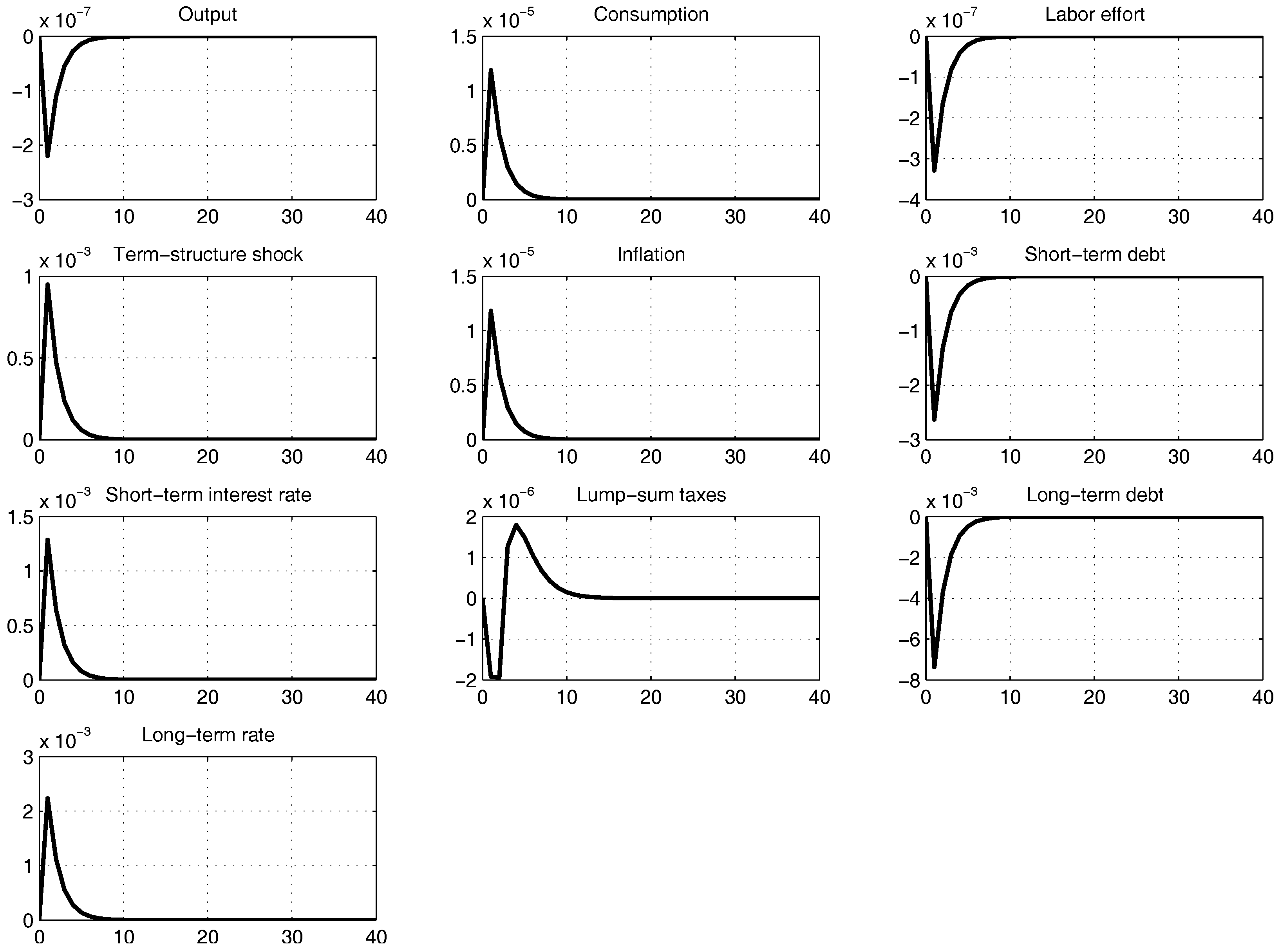
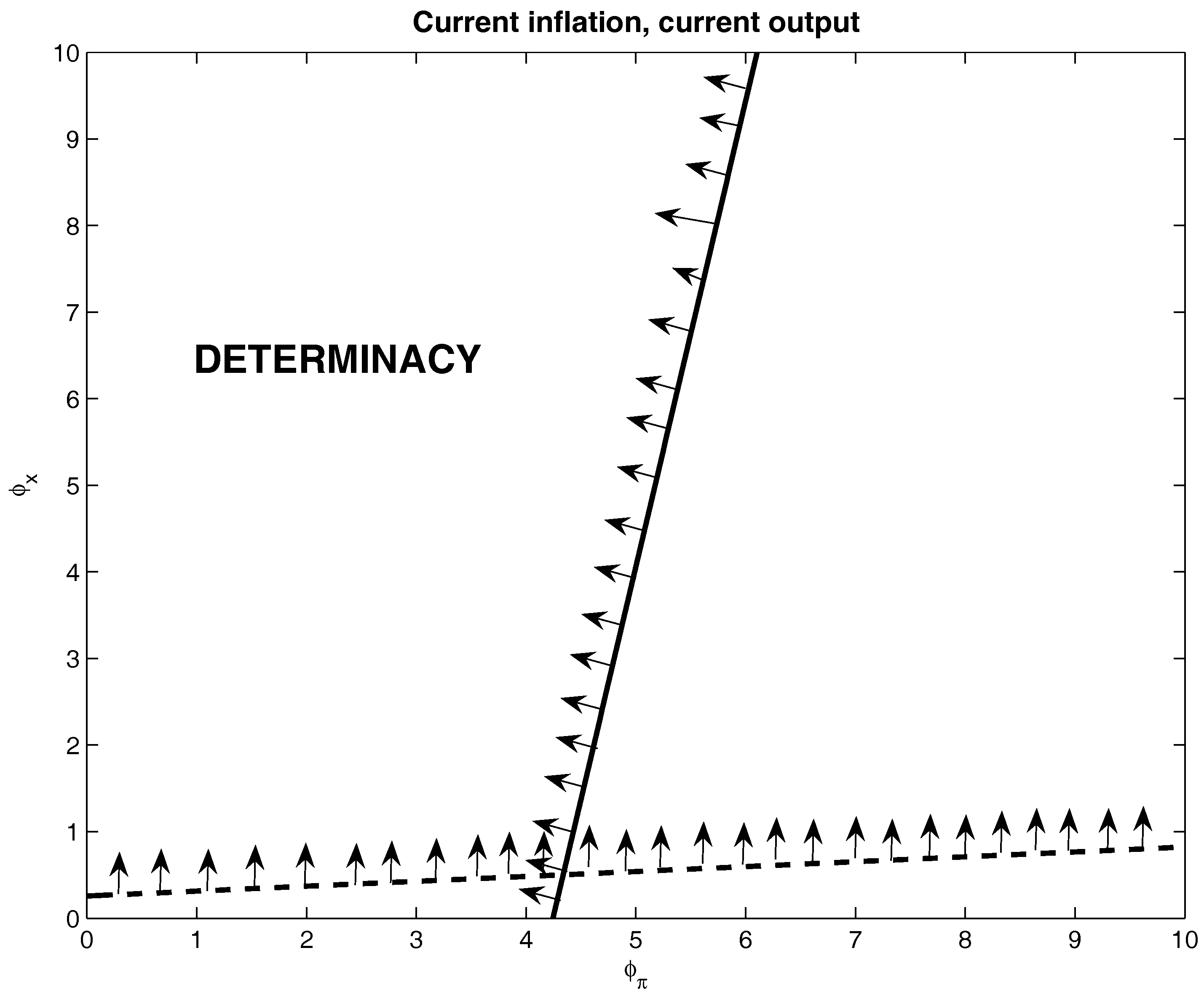
3.2. Pure Current-Inflation Targeting

In this section, we assume that monetary policy follows the simple rule
i ˜ t = ϕ π π ˜ t
The first-difference system is defined by the matrices
Z t = π ˜ t y ˜ t b ˜ t * ; A = β 0 0 λ i ϕ π λ π 1 0 a 1 γ y 1 ; B = 1 + μ i ϕ π μ y 0 γ i ϕ π 1 0 b 3 b 2 β 1 ψ 1
with a 1 γ i ϕ π + γ π ; b 2 γ i ϕ y + γ y ; b 3 θ i ϕ y + θ y , and
Γ = β 1 1 + μ i ϕ π β μ y 0 γ 21 γ 22 0 γ 31 γ 32 β 1 ψ 1
where the terms γ 21 , γ 22 , γ 31 , γ 32 in (31) are defined as follows
γ 21 = β 1 1 + μ i ϕ π λ π λ i ϕ π + γ i ϕ π γ 22 = 1 β 1 λ π λ i ϕ π γ 31 = γ y λ i ϕ π λ π γ i 1 + μ i ϕ π + b 3 a 1 γ i ϕ π
From (31), we observe that the structure of the system is block-triangular. Therefore, to study determinacy we can restrict our attention to the 2 × 2 submatrix Δ given by
Δ = β 1 1 + μ i ϕ π β μ y γ 21 γ 22
To achieve a fully-determinate system, two eigenvalues should be outside the unit circle and one inside, since public debt is a predetermined variable. This allows a richer configuration of determinacy conditions rather than in cases without an explicit role for the government budget constraint.
Proposition 2.
Let ϕ π 0 . Under contemporaneous pure inflation targeting rule, necessary and sufficient conditions for a rational expectations equilibrium to be determinate are:
(a) either
ϕ π > ϕ π 1 and β 1 1 < ψ 1 < β 1 + 1
(b) or
ϕ π < ϕ π 1 and ψ 1 < β 1 1 ; ψ 1 > β 1 + 1
where ϕ π 1 = μ y λ π 2 1 + β 2 μ i + μ y γ i + λ i .
Proof. 
See Appendix F. □
According to the terminology of Leeper (1991), condition (33) identifies a combination of active monetary and passive fiscal policy, while condition (34) identifies a combination of passive monetary and active fiscal. In the sense of Leeper (1991), an active monetary policy is defined when monetary authority sets nominal interest rate (or money supply) in order to keep under control the inflation rate. A passive monetary policy is when, instead, the interest rate (or money supply) are left free to adjust. In the recent monetary policy literature, condition (34) is identified with a combination of active fiscal policy and passive monetary policy. In particular, if ϕ π > ϕ π 1 and ψ 1 < β 1 1 , ψ 1 > β 1 + 1 , we have three roots inside the unit circle. In this case, we have three converging roots and a continuum of solution. In this case the price level is converging, but indeterminate. A combination of passive fiscal policy with passive monetary policy determines an indeterminacy of order 1. As condition (34) shows, determinacy can be also reached if the burden of price stability is entirely on behalf of fiscal policy authority. Hence, monetary policy can be also set independently from the inflation rate and determinacy is ensured by fiscal policy.

3.3. Expected Inflation Targeting

Now we consider a generalization of expected inflation targeting
i ˜ t = ϕ π E t π ˜ t + 1
The resulting system of first-order difference equations with the form (22) depends on the matrices14
A = 1 0 0 a 21 a 22 0 a 31 a 32 1 ; B = b 11 μ y b 11 0 0 1 0 0 θ y β 1 ψ 1
where a 21 = λ i ϕ π λ π β μ i ϕ π γ i ϕ π β μ i ϕ π β μ i ϕ π ; a 22 = β ϕ π μ i + λ i μ y β μ i ϕ π ; a 31 = γ π + γ i ϕ π β μ i ϕ π θ i ϕ π ; a 32 = γ y γ i ϕ π μ y β μ i ϕ π ; b 11 = β μ i ϕ π 1 . The structure of matrix Γ is given by
Γ = Γ 11 2 × 2 Γ 12 2 × 1 Γ 21 1 × 2 Γ 22 1 × 1 = = b 11 μ y b 11 0 a 21 b 11 a 22 μ y b 11 a 21 + 1 a 22 0 c 31 b 11 c 32 c 31 μ y b 11 + θ y β 1 ψ 1
where c 31 = a 21 a 32 a 22 a 31 / β ; c 32 = β 1 a 32 . From (36) we observe that the structure of the system is block-triangular. The conditions for determinacy are collected in the following proposition.
Proposition 3.
Given ϕ π 0 . For a model with expected inflation targeting interest rules, necessary and sufficient conditions for an equilibrium to be determinate are:
(i) either
ϕ ¯ π 1 < ϕ π < ϕ ¯ π 2 a n d β 1 1 < ψ 1 < β 1 + 1
(ii) or
ϕ ¯ π 1 < ϕ π < ϕ ¯ π 2 a n d ψ 1 < β 1 1 ; ψ 1 > β 1 + 1
Proof. 
See Appendix G. □
Proposition 3 suggests that it is possible to reach determinacy conditions without satisfying the Taylor principle. This is possible because of a non-trivial specification of the AS and IS curve, due to the different way by which liquidity services are modelled in this context.

3.4. Backward Inflation Targeting

Another variant of the Taylor rule is based on the idea of backward-looking inflation targeting
i ˜ t = ϕ π π ˜ t 1
Our results are collected in the following proposition
Proposition 4.
With a backward-looking rule, necessary and sufficient conditions for a unique equilibrium are such that
ϕ π > ϕ ¯ π 1
ϕ π > ϕ ¯ π 2
and
β 1 1 < ψ 1 < β 1 + 1
where
ϕ ¯ π 1 = λ π λ i γ i
ϕ ¯ π 2 = 1 + 2 1 + β + μ y λ π 2 μ i + μ y λ i + γ i
Proof. 
See Appendix H. □
With our baseline model calibration, the reader can easily check that bounds (43)–(44) are not binding, if ϕ π > 0 . As a result, the following holds:
Corollary 5.
With our model calibration, necessary and sufficient conditions for a unique equilibrium are ϕ π > 0 and (42).
This result emerges because the bounds established in Proposition 4 are negative. Obviously the determinacy regions depend on the parameter values of the Taylor rule. It should be stressed, though, that the Taylor principle does not need to hold strictly to generate determinate equilibria.

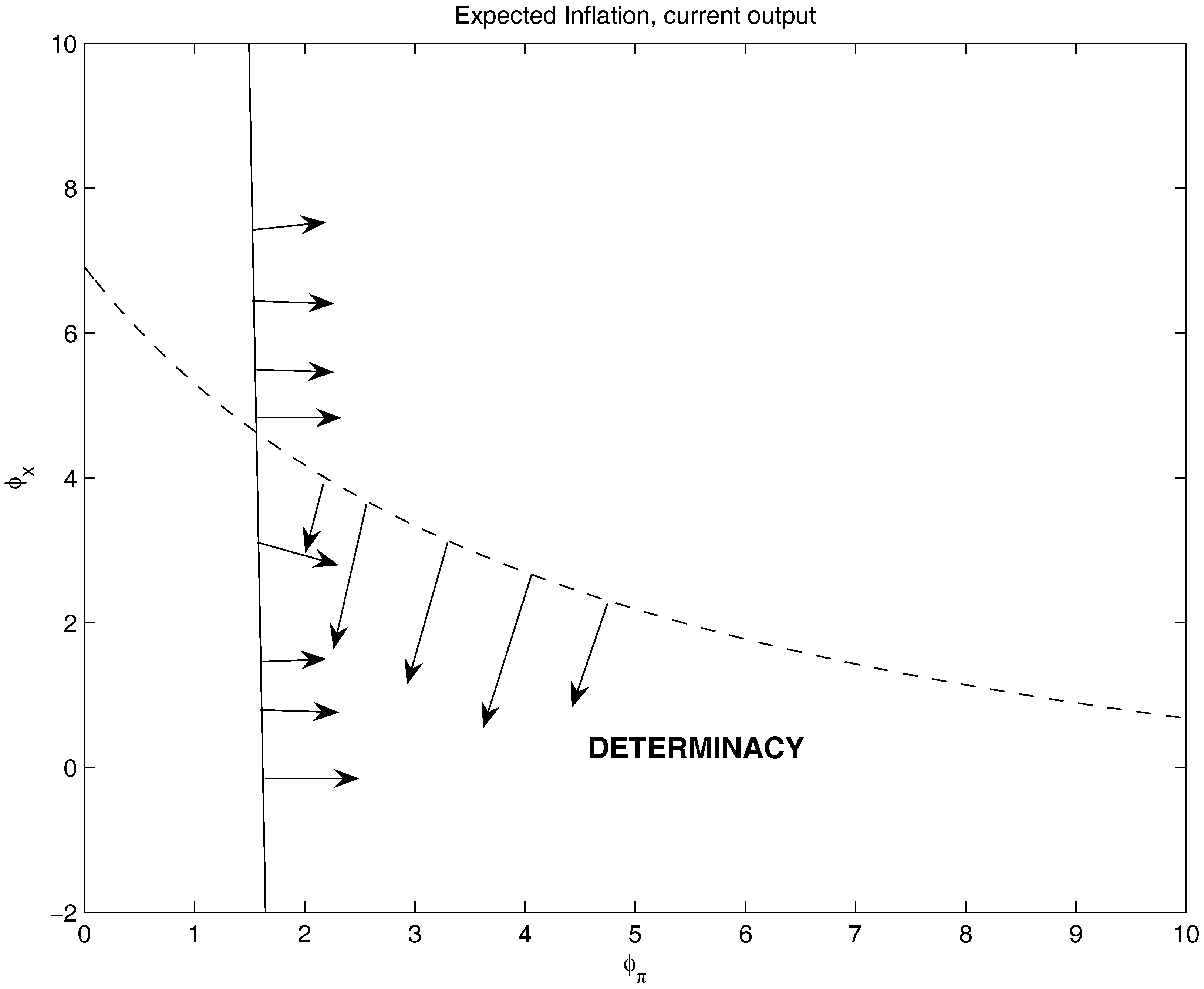
3.5. Expected Inflation and Current Output

In this section, we focus on the monetary policy rule
i ˜ t = ϕ π E t π ˜ t + 1 + ϕ y y ˜ t
Rule (45) is a representation for the monetary policy strategy of expected inflation targeting outlined by Svensson (2003). It is based on a pre-emptive response of the monetary authority with respect to the inflation rate.
Proposition 6.
Under rule (45), we have the following necessary and sufficient conditions for a unique equilibrium:
ϕ y < λ i μ y γ i μ i
ϕ π > β μ i
ϕ π > β γ i λ i μ i λ π γ i μ i
ϕ y < ϕ π μ i + μ y λ i γ i 1 β + μ y λ π 1 β λ i + μ i λ π ϕ π γ i μ i
and
β 1 1 < ψ 1 < β 1 + 1
Proof. 
See Appendix I. □
Figure 3 plots the numerical regions consistent with the bounds (48)–(49) for determinate equilibria. These are based on the model calibration discussed earlier. The continuous line refers to bound (48) for ϕ π , while the dashed line refers to (49) for ϕ y . We observe that the region for determinacy is located within an area for high values for ϕ π and low values for ϕ y . In this case, the conditions outlined above comply fully with the Taylor principle.

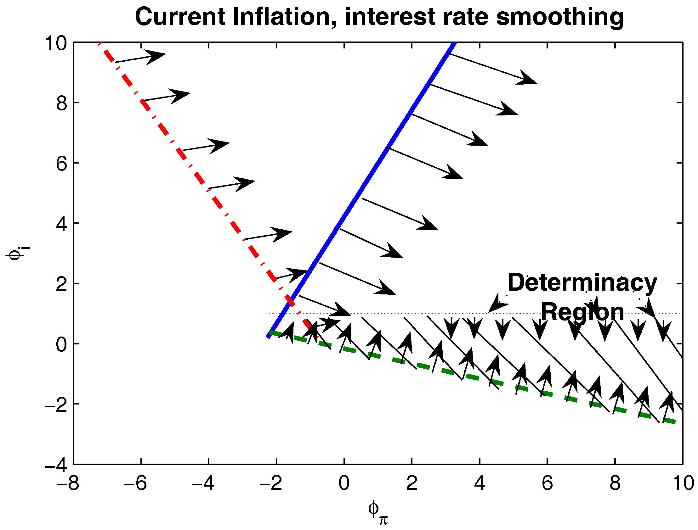
3.6. Interest-Rate Smoothing

Here we consider a Taylor rule with interest rate smoothing:
i ˜ t = ϕ π π ˜ t + ϕ i i ˜ t 1
The results are collected in the following proposition
Proposition 7.
Under Rule (51), the following necessary and sufficient conditions hold:
ϕ i < 1 β
ϕ π > 1 + β ϕ i μ y λ π β μ i + μ y γ i
ϕ π > μ y λ π 1 + β ϕ i 2 1 + β 2 β ϕ i 1 + β μ i 1 + β + μ y λ i + β γ i
ϕ i < ϕ π β μ i + μ y γ i 1 β μ y λ π
and
β 1 1 < ψ 1 < β 1 + 1
Proof. 
See Appendix J. □
Figure 4 plots the bounds described in Proposition 7 for the baseline calibration of the model. The horizontal line consists of the bound (52) for ϕ i . Proposition 7 establishes also two bounds for ϕ π . These follow from Equations (53) and (54) and are represented, respectively, by the= dash-dotted the dashed lines. The continuous line corresponds to the bound (55). From Figure 4 we observe that there are determinate equilibria for values of ϕ π generally bigger than one (as stated in the current empirical literature), and for values for ϕ i compatible with (52), when fiscal policy lies within the range defined by (56).

4. Conclusions

In this paper, we discuss the determinacy of equilibria in a cashless environment where government debt plays an important macroeconomic role. We consider a variant of the standard New Keynesian framework with two types of government bonds. We introduce a short-term bond that provides transaction services the purchase of consumption goods, and a long-term bond that acts as a store of value. We show that, when fiscal policy is designed according to the prescriptions of fiscal theory of the price level, determinacy is achieved by following the Taylor principle (see Leeper and Leith 2016). In order to pin down the price level, fiscal policy need not be passive in the sense of Leeper (1991). These findings confirm with those of Canzoneri and Diba (2005) and Canzoneri et al. (2008), who use a model with liquidity services from money and bonds to suggest that the Taylor principle is not a panacea for determinacy.
Our analysis can be extended along a number of relevant directions. First of all, we can drop the simplifying assumption about exogenous spread between the interest rates of the two types of bonds. An endogenous spread would introduce an additional element that might strengthen the macroeconomic role of government bonds and, possibly, alter the conditions for equilibrium determinacy. The introduction of different forms of distortionary taxation would add new transmission channel that can change the results greatly.
Vayanos and Vila (2009) has proposed a preferred-habitat theory of term structure of interest rates. Their work suggests that there is a non-negligible class of investors that have preference motives for holding government bonds with a desired maturity. But this opens up a specific scope for bonds in general equilibrium, which is independent from the role of transaction or liquidity services. In future work, we plan to consider an extended framework of substitutability or complementarity between consumption and government bonds.

Acknowledgments

This paper was previously distributed as a Bank of Finland Research Discussion Papers 24/2008 under the title “Determinacy of interest rate rules with bond transaction services in a cashless economy”. We are grateful to three anonymous referees for detailed comments. Refet Gürkaynak, Juha Kilponen, Michael Plummer, Ulf Söderström and Jouko Vilmunen deserve a special mention for many discussions and suggestions that shaped the paper greatly.

Author Contributions

This paper is the result of joint work by both authors since its earlier publication as a Bank of Finland Discussion Paper.

Conflicts of Interest

The authors declare no conflicts of interest.

Appendix A. A Further Discussion on Model Structure and Equilibrium Conditions

In this section, we provide a further discussion on the model structure, the first-order conditions, and the regularity conditions that characterize the bond-velocity term.

Appendix A.1. Supply Side

Each individual firm faces a downward demand curve of the same sort of (A11), with Y t j in place of C i t and chooses the optimal quantity of labour input L t j by maximizing the following stream of real profits
Ω t j = t = 0 ρ t ω t j = t = 0 ρ t P t j P t Y t j W t P t L t j A C t p
subject to the demand function (A11), to the production function (16) and to the price adjustment cost function (15). Note that in (A1) ρ t is a stochastic pricing kernel for contingent claims employed by firms to discount future profit stream. Thus, the firm’s first order condition with respect to L t j is
W t P t = α 1 1 ψ t j Y t j L t j P t j P t
with
1 ψ t j = 1 θ 1 ϕ p P t j P t 1 j π P t P t 1 j Y t Y t j + E t ϕ p ρ t + 1 ρ t P t + 1 j P t j π P t + 1 P t j P t + 1 j P t j Y t + 1 Y t j
The term ψ t j can be interpreted as the output demand elasticity augmented by cost of price adjustment weighted by the stochastic pricing kernel ρ t . In steady state, if P t j P t 1 j = π for all t and j, we get that ψ t j = θ . The markup for each firm j is defined by
μ t j = 1 1 ψ t j 1
In steady state, the markup is given by θ θ 1 , so that when θ , μ 1 . With perfectly flexible prices with ϕ p = 0 the markup is once again θ θ 1 . From the expressions in (A3)–(A4) we see that that markup becomes endogenous and works as a transmission channel for both real and nominal shocks. An increase in ψ t j reduces μ t j and is expansionary, due to the reduction of monopolistic distortion.

Appendix A.2. Demand Side

An important aspect for a full characterization of the equilibrium is represented by the role of intertemporal discount factor of both firms and consumers. In what follows, we assume that each agent has access to a set of complete market for contingent claims. The direct implication of this assumption is that the discount factor of households should equal that of firms, as stated by:
ρ t + 1 ρ t = β λ t + 1 λ t
For the intuition behind condition (A5) it is enough to imagine the presence of a representative agent who can freely exchange shares of each firm, without paying any transaction cost. The same result can be obtained by including an additional first order condition for the optimal allocation of shares for the representative agent.
By combining the first-order conditions on consumption and labour (6)–(7) together with (10), the labour supply curve is given by
1 γ γ C t 1 L t = W t 1 + χ 2 F t 2 + χ F t
From Equation (A6) it is not difficult to show that the labour supply function is increasing with respect to real wage, but decreasing with respect to consumption. After making use of the equation of the government budget constraint, we find the following expression for the aggregate resource equation
C t 1 + χ 2 F t 2 = Y t 1 ϕ p 2 π t π 2 G t
From (A7) we observe that the amount of income available for consumption is obtained net of resources employed for making transactions and public expenditure. An important feature considered in the present model derives from the specific functional form assumed for the transaction costs function (10). In fact, from Euler Equation (9) we find that
1 + i t β λ t + 1 π t = λ t 1 χ F t 3
where, from (6) λ t is defined according to
λ t = C t γ 1 1 σ 1 1 L t 1 γ 1 1 σ 1 + χ 2 F t 2 + χ F t P t
Therefore, since λ t is a monotone decreasing function of F t , there are at least two positive steady state satisfying (A8). The first is such that λ = 0 , with F = . The second is given by
1 + i β π = 1 χ F 3
There might be no solution to Equation (A10). This is the case if 1 + i β > π . In what follows, we assume that 1 + i β < π . If this condition is verified, we immediately get that Equation (A8) becomes a difference equation, with a converging solution.
The standard optimization problem for the choice of the optimal composition of bundle (14) leads to the following constant-elasticity inverse demand function
c t i j C t = p t j P t θ
where p t j is the price of variety j and P t is the general price index defined as
P t = 0 1 p t j 1 θ d j 1 1 θ
As θ demand function becomes perfectly elastic, and the differentiated goods are perfect substitutes. The aggregate price level P t is beyond the control of each individual firm. When we aggregate C t and c t i j across all agents i , we find the aggregate demand for final goods and for variety j, given respectively by Y t = 0 1 C t d i and Y j t = 0 1 c t i j d i , for all j 0 , 1 .

Appendix A.3. Some Considerations on the Bond-Velocity Term

In what follows, we aare going to sketch an argument in order to exclude that the ‘bond velocity’ term F grows arbitrarily without bound with positive probability. The discussion and notation is based on a similar argument proposed by Sims (1994) in a monetary model.
Let F be the unique solution to (A10). If we have an off-equilibrium path value for F t such that F t > F or β < π , then from Equation (A8) we find that
E t λ t + 1 < Φ λ t
for a given Φ , such that 0 < Φ < 1 . Therefore, given the information available at time t condensed by the information set I t , the probability that λ t + 1 is lower than λ t is positive, given Equation (A13), namely
P λ t + 1 < Φ λ t I t > 0
Applying (A14) recursively, we get
P λ t + s < Φ s λ t I t > 0
Equation (A14) together with the transaction technology function puts an upper bound on F. This allows to exclude any path for λ t that require F growing with positive probability. To sum up, if F t > F for all t, then λ t must have a positive probability of growing arbitrarily close to zero as t . However, this would imply a non-zero probability of arbitrarily large values of F t . Therefore, F t > F is impossible on an equilibrium path. By a similar argument, if β > π , we have a positive probability of getting an arbitrarily large large value of F, which is inconsistent with an equilibrium positive level of unstarred debt.
By the same sort of argument, if F t < F , for some t and β > π we have that there is a non-zero probability that λ t + s becomes arbitrarily large, so F t assumes values arbitrarily close to zero, as t . This is once again inconsistent with the equilibrium path, because it violates the transversality condition. Again, we must conclude that the value for F which solves (A10) is an equilibrium value.

Appendix B. The Log-Linearized Model

The next step consists in reducing the model into a three equations system, an intertemporal version of the IS equation, an aggregate supply equation (AS, henceforth), and the government budget constraint. In order to derive the reduced form system, we take a log-linear approximation around the steady state. In what follows, each variable y ˜ t is approximated around the steady state by using the formula X ˜ t = log y ˜ t log X . Via recursive substitution, we arrive at the following log-linearized version of the resource constraint
C ˜ t = Y ˜ t S c 1 + χ F 2 g S c 1 + χ F 2 G ˜ t 2 S c χ F 3 b ζ S c 1 + χ F 2 ζ ˜ t + 2 S c χ F 2 b i S c 1 + χ F 2 i ˜ t
where the coefficients b ζ and b i , are reported in Appendix C. The next step consists in log-linearizing the first order conditions (6) and (7), eliminate C ˜ t from both equation, by making use of (A16). Next, we can eliminate L ˜ t from the log-linearized version of the production function to get the following equation for λ ˜ t
λ ˜ t = η y Y ˜ t η g G ˜ t + η a A ˜ t + η ζ ζ ˜ t + η i i ˜ t
where the analytical expression for the coefficients η y , η g , η a , η ζ , η i are reported in Appendix C.
After having log-linearized the first order condition on B t * (Equation (8)), the intertemporal IS equation (after rearrangement) is
Y ˜ t + 1 λ g G ˜ t + 1 + λ a A ˜ t + 1 + λ ζ ζ ˜ t + 1 + λ i i ˜ t + 1 λ π π ˜ t + 1 = Y ˜ t λ g G ˜ t + λ a A ˜ t + γ ζ ζ ˜ t + γ i i ˜ t
where the coefficients are defined as λ g = η g / η y , λ a = η a / η y , λ ζ = η ζ / η y , λ i = η i / η y , γ ζ = η ζ α i η y 1 , λ π = η y 1 . Equation (A18) is the intertemporal IS equation, as discussed by Rotemberg and Woodford (1997), among others. The new feature expressed in Equation (A18) is given by the presence of the nominal interest rate dated at time t + 1 , i ˜ t + 1 , together with the interest rate dated at time t, i ˜ t . The presence of i ˜ t + 1 is due to the characteristics of the transaction technologies F and B considered in the model.
The derivation of the aggregate supply equation starts from the log-linearization of the elasticity ψ t given by
ψ ˜ t = ϕ p π ˜ t β ϕ p π ˜ t + 1
To simplify algebra, we assume that the steady state of the inflation rate has been set equal to 1. From the first order condition with respect to L we have that
W ˜ t = Y ˜ t L ˜ t + θ 1 1 ϕ p π ˜ t θ 1 1 β ϕ p π ˜ t + 1
Moreover, from the production function L ˜ t = α 1 Y ˜ t A ˜ t . To get an useful expression of the AS equation, we can substitute out into the log-linearized version of (7), the Equation (A20) for W ˜ t , Equation (A17) for λ ˜ t , Equation (A16) for C ˜ t , and L ˜ t . After rearrangement, we find
β E t π ˜ t + 1 = π ˜ t μ y Y ˜ t + μ g G ˜ t + μ ζ ζ ˜ t + μ A A ˜ t + μ i i ˜ t
where the coefficients μ y , μ g , μ A , μ ζ , μ i are reported in Appendix C.
The model is expressed as a function of the output gap y ˜ t defined (in log-linear terms) as X ˜ t = Y ˜ t Y ˜ t p , where Y ˜ t p is the level of potential output defined as
Y ˜ t p = μ g μ y G ˜ t + μ ζ μ y ζ ˜ t + μ A μ y A ˜ t
Therefore, the aggregate supply equation can be written as
β E t π ˜ t + 1 = π ˜ t μ y X ˜ t + μ i i ˜ t
By the same sort of argument, we can rewrite also the IS equation by using the definition of the output gap given by (A22), to get
X ˜ t + 1 + λ i i ˜ t + 1 λ π π ˜ t + 1 = X ˜ t + γ i i ˜ t + R t n
where R t n indicates a composite term of disturbances defined as follows
R t n = δ g G ˜ t G ˜ t + 1 + δ a A ˜ t A ˜ t + 1 + δ ζ 2 ζ ˜ t δ ζ ζ ˜ t + 1
The term R t n defined in (A25) indicates the natural rate of interest, namely the real interest rate consistent with full employment equilibrium and a zero inflation rate. In the definition of R t n there are all the stochastic processes of the model. It should be stressed, though, R t n is an irrelevant term for the purpose of the determinacy analysis because its magnitude does not affect the dynamic structure of the model. Differently from the standard AS equation proposed in the literature, Equation (A23) includes the nominal interest rate i ˜ t . This is due to the relationship between the level of real debt b t and the nominal interest rate.
Since we study the issue of price level determination in relation to fiscal solvency, a key equation of the above system is the government budget constraint. In order to make the system entirely defined by four variables (inflation rate, output gap, interest rate and unstarred real debt), we can now derive the semi-reduced form of the government budget constraint
γ y X ˜ t + b ˜ t * + γ π π ˜ t + γ i i ˜ t = β 1 ψ 1 b ˜ t 1 * + θ i i ˜ t 1 + θ y X ˜ t 1 + R 2 t
where R 2 t is
R 2 t = θ g + θ y μ g μ y G ˜ t 1 γ g G ˜ t + θ y μ a μ y A ˜ t 1 γ y μ a μ y A ˜ t + θ ζ + θ y μ ζ μ y ζ ˜ t 1 γ ζ ζ ˜ t
with the coefficients reported in the following appendix.

Appendix C. Coefficients of the Reduced-Form Model

b ζ = ζ i 3 χ F 3 1 + ζ i ; b i = i 1 ζ + ζ i 2 3 χ F 3 1 + ζ i 2
Coefficients of Equation (A17)
η y = γ 1 1 σ 1 S c 1 + χ F 2 1 γ 1 1 σ L α 1 L ; η a = 1 γ 1 1 σ L α 1 L ; η ζ = χ F 1 + F b ζ 1 + χ 2 F 2 + χ F γ 1 1 σ 1 2 S c χ F 2 b ζ S c 1 + χ F 2 ; η g = γ 1 1 σ 1 g S c 1 + χ F 2 ; η i = γ 1 1 σ 1 2 S c χ F 2 b i S c 1 + χ F 2 χ F 1 + F 1 + χ 2 F 2 + χ F
Coefficients of Equation (A21):
μ y = θ 1 ϕ p γ 1 1 σ S c 1 + χ F 2 1 γ 1 1 σ 1 L 1 L 1 α η y 1 μ g = θ 1 ϕ p γ 1 1 σ g S c 1 + χ F 2 η g μ i = θ 1 ϕ p η i 2 S c χ F 2 b i γ S c 1 + χ F 2 1 1 σ μ ζ = θ 1 ϕ p η ς + 2 S c χ F 2 b ζ γ S c 1 + χ F 2 1 1 σ μ A = θ 1 ϕ p η A 1 γ 1 1 σ 1 L 1 L 1 α
The coefficients of Equation (A26) are defined as:
γ y = b b * 1 S c 1 + χ F 2 ; γ ζ = b b * 2 χ F 3 b ζ 1 + χ F 2 α i = 2 χ F 2 b i 1 + χ F 2 ; γ i = b b * α i ; γ g = 1 b * b g S c 1 + χ F 2 + G θ i = i * + i b b * + 1 + i b α i b * + b b * 2 χ F 2 b i ψ 2 1 + χ F 2 + ψ 2 b b i b * γ π = i * + i b b * ψ 1 ψ 2 b b * θ ζ = i * 1 + i b b * 2 χ F 3 b ζ 1 + χ F 2 + 2 b χ F 3 b ζ ψ 2 b * 1 + χ F 2 ψ 2 b b ζ b * θ y = b 1 + i ψ 2 b * S c 1 + χ F 2 ; θ g = b ψ 2 1 + i g b * S c 1 + χ F 2

Appendix D. Schur-Cohn Criterion

Appendix D.1. 2 × 2 Matrix

The characteristic equation of a 2 × 2 matrix A is given by x 2 t r ( A ) x + det ( A ) = 0 . It is well known that the condition for two roots of the characteristic equation to lie outside the unit circle is (see LaSalle 1986):
det ( A ) > 1 ,
t r ( A ) < 1 + det ( A ) .
In particular, condition (A29) can be split up in the following two inequalities:
1 + det ( A ) + t r ( A ) > 0
1 + det ( A ) t r ( A ) > 0

Appendix D.2. 3 × 3 Matrix

In what follows, to facilitate the task of the reader, we present the entire set of conditions to be satisfied by a generic 3 × 3 matrix B in order to have one root inside the unit circle and two roots outside the unit circle. Given the following characteristic polynomial of a 3 × 3 matrix:
λ = λ 3 + A 2 λ 2 + A 1 λ + A 0
where: A 0 = d e t B ; A 1 = t r B ; A 2 = Ω B = b 11 b 22 b 21 b 12 + b 22 b 33 b 32 b 23 + b 11 b 33 b 31 b 13 . Therefore, necessary and sufficient conditions are given by the following restrictions on the coefficients of the characteristic polynomial (A32). Either:
CASE I
1 + A 2 + A 1 + A 0 < 0
1 + A 2 A 1 + A 0 > 0
or:
CASE II
1 + A 2 + A 1 + A 0 > 0
1 + A 2 A 1 + A 0 < 0
A 0 2 A 0 A 2 + A 1 1 > 0
or:
CASE III
1 + A 2 + A 1 + A 0 > 0
1 + A 2 A 1 + A 0 < 0
A 0 2 A 0 A 2 + A 1 1 < 0
A 2 > 3

Appendix E. Proof of Proposition 1

The trace and the determinant of submatrix Δ defined in (32) are:
det Δ = 1 β + μ i + μ y γ i ϕ π β t r Δ = 1 + 1 β + μ i + μ y γ i ϕ π β μ y λ π β
From condition (A28) of the Schur-Cohn criterion, it is certainly true that det Δ > 1 . The condition det Δ > 1 implies:
ϕ π > 1 β μ i + μ y γ i
On the other hand, condition (A30) directly implies:
ϕ π > μ y λ π 2 1 + β 2 μ i + μ y γ i + λ i
while (A31) implies:
ϕ π 1 + γ i λ i > 0
which is always satisfied, since we set ϕ π > 0 , by hypothesis. By using the benchmark parameter values considered in the model, it is immediate to verify that the bound established by (A43) is bigger than that specified by (A42), under a wide range of the core parameter values. Therefore, condition (A43) is both necessary and sufficient to ensure determinacy.
For the system condensed in matrix Γ we require that the third root be inside the unit circle. This is true if
β 1 ψ 1 < 1 ,
which means that fiscal policy is passive according to Leeper (1991). This condition is equivalent to:
β 1 1 < ψ 1 < β 1 + 1
When both conditions (A43) and (A46) are satisfied, then all the three roots of the system are inside the unit circle, and the equilibrium will be unique. □

Appendix F. Proof of Proposition 2

Once again, given the triangular structure of matrix we can concentrate on the eigenvalues of the submatrix Γ 11 2 × 2 and that of Γ 22 1 × 1 , in (24)–(25).
The trace and the determinant of submatrix Γ 11 2 × 2 are given, respectively, by:
t r Γ 11 = 1 + μ i ϕ π 1 + λ i ϕ y + λ π λ i ϕ π μ i ϕ y μ y + β 1 + γ i ϕ y β 1 + λ i ϕ y det Γ 11 = μ i ϕ π + 1 + γ i ϕ y μ y β 1 + λ i ϕ y
The condition det Δ > 1 implies:
ϕ π > μ y 1 β γ i β λ i ϕ y μ i
On the other hand, from condition (A30) we get:
ϕ π > μ y 1 + λ π 2 1 + β ϕ y λ i + λ π μ i + γ i 1 + β 2 μ i + λ i μ y
Finally, from (A31) we find the following bound:
ϕ y > ϕ π λ i μ i + β 1 + μ y 1 λ π γ i λ i λ π μ i β γ i
According to benchmark parameter values in the calibration section, we immediately get that the bounds which are only binding are (A48) and (A49). In fact, bound given by (A47) is negative, given our parameter values so it is not binding by setting ϕ π > 0 .
Condition (A48)–(A49) imply that two eigenvalues of matrix Γ are outside the unit circle: this is enough to establish the equilibrium determinacy induced by rule (21). Thus, the third root given by the determinant of Γ 22 1 × 1 should lie inside the unit circle. This is equivalent to require that condition (A45) be verified, or that β 1 1 < ψ 1 < β 1 + 1 , which directly originates condition (26).
If one of the two bounds given in (A48)–(A49) is not respected—for example, the lower bound given by (A48)—then the submatrix Γ 11 will have one root inside and one outside the unit circle. To restore determinacy we need another root outside the unit circle: this can be reach by setting β 1 ψ 1 > 1 , or ψ 1 < β 1 1 ; ψ 1 > β 1 + 1 . □

Appendix G. Proof of Proposition 3

Therefore, to study determinacy we can focus on the 2 × 2 submatrix Δ 2 × 2 given by
Δ = b 11 μ y b 11 a 21 b 11 a 22 μ y b 11 a 21 + 1 a 22
The determinant and trace of matrix Δ are given, respectively, by:
det Δ = 1 β ϕ π μ i + λ i μ y trace Δ = 1 μ y λ π + β μ i ϕ π μ y γ i ϕ π β ϕ π μ i + λ i μ y
To study determinacy, we require conditions (A28)–(A29) to be satisfied. From (A28) we find that det Δ > 1 can be satisfied if:
ϕ π > 1 β μ i + λ i μ y = ϕ ¯ π 1
while condition det Δ < 1 implies:
ϕ π > 1 + β μ i + λ i μ y
Condition (A52) is satisfied by setting ϕ π > 0 . The second set of condition (A29) can be split into (A30)–(A31). From (A30) we get:
ϕ π < 2 1 + β λ π μ y 2 μ i + μ y λ i + γ i = ϕ ¯ π 2
while from (A31) we have that:
ϕ π > λ π γ i λ i = ϕ ¯ π 3
To get determinacy (one root inside and one root outside the unit circle), we require:
ϕ ¯ π 1 < ϕ π < ϕ ¯ π 2
Condition (A55) implies that two roots of submatrix (A50) are outside the unit circle. On the other hand, the third root of the whole matrix (36) has to be outside the unit circle: this is obtained by fixing parameter ψ 1 within the range β 1 1 < ψ 1 < β 1 + 1 . If (A55) is not satisfied, this means that only one root of the submatrix (A50) is outside the unit circle. To fulfill the requirement that two roots of (36) have to stay outside the unit circle we must require that β 1 ψ 1 > 1 .

Appendix H. Proof of Proposition 4

The system can be cast in the same format as in (23), where vector Z t is now given by Z t = i ˜ t , π ˜ t , y ˜ t , b ˜ t * , matrix Γ is:
Γ = 0 Δ 3 × 3 0 0 c 41 c 42 c 43 β 1 ψ 1
where submatrix Δ 3 × 3 is:
Δ 3 × 3 = 0 ϕ π 0 μ i β 1 β μ y β λ π μ i β + γ i λ π β λ i ϕ π 1 λ π μ y β
det Δ = ϕ π β μ y γ i + μ i ; t r Δ = 1 + 1 β μ y λ π β ; Ω = 1 ϕ π λ i μ y μ i ϕ π β . To study determinacy, we require that matrix (A56) to have two roots outside and two roots inside the unit circle. Given the block-triangular structure of the model, we require submatrix (A57) to have two roots inside and one root outside the circle. To verify this, we can apply conditions (A33)–(A34). Condition (A33) implies:
ϕ π > λ π λ i γ i = ϕ ¯ π 1
From condition (A34), we find (after proper rearrangments):
ϕ π > 1 + 2 1 + β + μ y λ π 2 μ i + μ y λ i + γ i = ϕ ¯ π 2
On the other hand, the fourth root of the whole matrix (36) has to be outside the unit circle: this is obtained by fixing parameter ψ 1 within the range β 1 1 < ψ 1 < β 1 + 1 . If (A58) or (A59) are not satisfied, then only one root of the submatrix (A50) is outside the unit circle. To fulfill the requirement that two roots of (36) have to stay outside the unit circle we must require that β 1 ψ 1 > 1 .

Appendix I. Proof of Proposition 6

By using the rule (45) in (A23), (A24), (A26) and rearranging, we find that the system can be cast in the same format as in (23), with vector Z t given by Z t = π t , y ˜ t , b t * , and matrix Γ is
Γ = a 1 a 2 0 a 1 b 2 b 1 1 b 1 1 a 2 b 2 + b 3 0 c 31 a 1 a 2 c 31 + b 3 c 32 + d 3 β 1 ψ 1
where a 1 = β μ i ϕ π 1 ; a 2 = μ y μ i ϕ y β μ i ϕ π 1 ;
b 1 = 1 + λ i ϕ y λ i ϕ π μ y μ i ϕ y β μ i ϕ π 1 ;
b 2 = λ i ϕ π β μ i ϕ π 1 λ π γ i ϕ π ; b 3 = 1 + γ i ϕ y ;
d 1 = γ y θ i ϕ π μ y μ i ϕ y β μ i ϕ π 1 + γ i ϕ y ; d 2 = γ π + γ i ϕ π β μ i ϕ π 1 θ i ϕ π ;
d 3 = θ i ϕ y + θ y ; c 31 = b 2 d 1 b 1 1 d 2 ; c 32 = d 1 b 1 1
Given the block triangularity structure of matrix (A60), we can concentrate on the submatrix Δ
Δ = a 1 a 2 a 1 b 2 b 1 1 b 1 1 a 2 b 2 + b 3
The system considered in matrix (A60) has a determinate solution if and only if two roots are outside and one inside the unit circle. By applying (A28) to matrix (A61), we find that condition det Δ > 1 , implies:
β ϕ y γ i λ i + ϕ π λ i μ y γ i μ i ϕ y > 0
which is verified if and only if:
ϕ y < λ i μ y γ i μ i
since ϕ π > 0 by hypothesis and γ i > λ i , by construction. Condition det Δ < 1 implies (after rearrangements):
ϕ π > β μ i
Furthermore, condition (A30) implies:
ϕ π ϕ y μ i β γ i λ i μ i λ π + ϕ π γ i + β μ i ϕ π λ i ϕ y 1 + β 1 + β μ y λ π + 1 + β ϕ π μ y γ i + λ i + μ i > 0
Since μ i < 0 (from parameters value) and (A62), to satisfy (A63) we require that
c c β γ i λ i μ i λ π + ϕ π γ i < 0
λ i ϕ y 1 + β 1 + β μ y λ π + 1 + β ϕ π μ y γ i + λ i + μ i < 0
From (A64), we find:
ϕ π > β γ i λ i μ i λ π γ i μ i
from (A65), we have, instead:
ϕ π > λ i ϕ y 1 + β 1 + β μ y λ π + 1 + β μ y γ i + λ i + μ i
From condition (A31), we have that:
ϕ π μ i 1 + ϕ y γ i + μ y γ i λ i > 1 β μ y λ π + ϕ y 1 β λ i + μ i λ π
which gives the following bound:
ϕ y < ϕ π μ i 1 + ϕ y γ i + μ y γ i λ i 1 β + μ y λ π 1 β λ i + μ i λ π
as stated. The condition relative to the fiscal side of the model are still the same as those considered in the previous propositions.

Appendix J. Proof of Proposition 7

The system can be cast in the same format as in (23), where vector Z t is now Z t = i ˜ t , π ˜ t , y ˜ t , b ˜ t * , matrix Γ is:
Γ = 0 Δ 3 × 3 0 0 h 41 h 42 h 43 β 1 ψ 1
where:
Δ 3 × 3 = ϕ i + μ i ϕ π β ϕ π β μ y ϕ π β μ i β 1 β μ y β λ i ϕ i + μ i λ π ϕ π λ i β λ π ϕ π λ i β 1 μ y λ π ϕ π λ i β
with:
  • h 41 = d 41 ϕ i + d 42 μ i + γ y γ i + θ i ; h 42 = d 42 ;
  • h 43 = μ y d 42 + γ y + θ y ; d 42 = γ i ϕ π β + γ π β + γ y β λ π ϕ π λ i .
To obtain determinacy, we need to have two roots inside the unit circle and two roots outside. Let us concentrate on the characteristics of matrix (A70). In order to find conditions that ensure matrix (A70) to have one root inside and one outside unit circle, we need to study which of the three cases apply to polynomial. In this case, we have that:
A 2 = t r ( Δ ) = β ϕ i + μ i ϕ π + 1 + β μ y λ π ϕ π λ i A 1 = β ϕ i 1 + β + β β ϕ i μ y λ π + μ i ϕ π β + μ y ϕ π β γ i A 0 = β 2 ϕ i
According to (A33) from Case I, we get:
μ i ϕ π β 1 + μ y λ π 1 β ϕ i + μ y ϕ π β γ i λ i < 0
From current parameter values, it is not difficult to check that condition (A71) is not satisfied. Therefore, we apply conditions (A35)–(A37) from Case II. Condition (A71) is satisfied with reversed sign if and only if:
1 β > ϕ i
From (A36) we have:
ϕ π > μ y λ π 1 + β ϕ i 2 1 + β 2 β ϕ i 1 + β μ i 1 + β + μ y λ i + β γ i
Consider now condition (A37) to get the following bound:
β 2 ϕ i 1 + β 2 + β 1 + ϕ i + β 2 ϕ i β ϕ i + μ i ϕ π + 1 + β μ y λ π ϕ π λ i + + μ i ϕ π β β ϕ i μ y λ π + β ϕ π μ y γ i 1 > 0
We observe that β 2 ϕ i 1 + β 2 + β 1 + ϕ i is positive by definition. The expression in squared brackets of (A74) is positive if and only if:
ϕ π > μ y λ π 1 β 1 + ϕ i μ i + μ y λ i
The last part of Equation (A74) is positive if and only if
ϕ i < ϕ π β μ i + μ y γ i 1 β μ y λ π

References

  1. Aggarwal, Reena, Jennie Bai, and Luc Laeven. 2017. Safe Asset Shortages: Evidence from the European Government Bond Lending Market. Unpublished paper. August. [Google Scholar]
  2. Bernanke, Ben. 2008. Federal Reserve Policies in the Financial Crisis. Austin: The Greater Austin Chamber of Commerce, December 1. [Google Scholar]
  3. Bowman, David, Etienne Gagnon, and Mike Leahy. 2010. Interest on Excess Reserves as a Monetary Policy Instrument: The Experience of Foreign Central Banks; International Financial Discussion Paper No. 996; Washington: Federal Reserve Board.
  4. Canzoneri, Matthew B., and Behzad T. Diba. 2005. Interest Rate Rules and Price Determinacy: The Role of Transactions Services of Bonds. Journal of Monetary Economics 52: 329–43. [Google Scholar] [CrossRef]
  5. Canzoneri, Matthew B., Robert Cumby, Behzad Diba, and J. David Lopez-Salido. 2008. Monetary and Fiscal Policy Coordination when Bonds Provide Transaction Services. CEPRWorking Paper No. 6814. London, UK. [Google Scholar]
  6. Canzoneri, Matthew B., Robert Cumby, Behzad Diba, and J. David Lopez-Salido. 2011. The role of liquid government bonds in the great transformation of American monetary policy. Journal of Economic Dynamics and Control 35: 282–94. [Google Scholar] [CrossRef]
  7. Cochrane, John H. 2014. Monetary Policy with Interest on Reserves. Journal of Economic Dynamics and Control 49: 74–108. [Google Scholar] [CrossRef]
  8. Clarida, Richard, Jordi Galì, and Mark Gertler. 2000. Monetary Policy Rules and Macroeconomic Stability: Evidence and Some Theory. Quarterly Journal of Economics 115: 147–80. [Google Scholar] [CrossRef]
  9. Dixit, Avinash K., and Joseph Stiglitz. 1977. Monopolistic Competition and Optimum Product Diversity. American Economic Review 67: 297–308. [Google Scholar]
  10. Feenstra, Robert C. 1986. Functional Equivalence Between Liquidity Costs and the Utility of Money. Journal of Monetary Economics 17: 271–91. [Google Scholar] [CrossRef]
  11. Gagnon, Joseph, Matthew Raskin, Julie Remache, and Brian Sack. 2010. Large-Scale Asset Purchases by the Federal Reserve: Did They Work? Federal Reserve Bank of New York Staff Report. No. 441.
  12. LaSalle, Joseph P. 1986. The Stability and Control of Discrete Processes. New York and Berlin: Springer Verlag. [Google Scholar]
  13. Leeper, Eric M. 1991. Equilibria Under Active and Passive Monetary and Fiscal Policies. Journal of Monetary Economics 27: 129–47. [Google Scholar] [CrossRef]
  14. Leeper, Eric M., and Campbell Leith. 2016. Understanding Inflation as a Joint Monetary-Fiscal Phenomenon; NBER Working Papers, No. 21867; Cambridge: National Bureau of Economic Research.
  15. Rotemberg, Julio J. 1982. Sticky Prices in the United States. Journal of Political Economy 90: 1187–211. [Google Scholar] [CrossRef]
  16. Rotemberg, Julio J., and Michael Woodford. 1997. An Optimization-Based Econometric Framework for the Evaluation of Monetary Policy. In NBER Macroeconomic Annual. Edited by Ben Bernanke and Michael Woodford. Cambridge: The MIT Press. [Google Scholar]
  17. Sims, Christopher A. 1994. A Simple Model for Study of the Determination of the Price Level and the Interaction of Monetary and Fiscal Policy. Economic Theory 4: 381–99. [Google Scholar] [CrossRef]
  18. Taylor, John B. 1993. Discretion versus Policy Rules in Practice. In Carnegie-Rochester Conference Series on Public Policy. Amsterdam: Elsevier, vol. 39, pp. 195–214. [Google Scholar]
  19. Vayanos, Dimitri, and Jean-Luc Vila. 2009. A Preferred-Habitat Model of the Term Structure of Interest Rates; NBER Working Paper, No. 15487; Cambridge: National Bureau of Economic Research.
  20. Vayanos, Dimitri, and Jean-Luc Vila. 1999. Equilibrium Interest Rate and Liquidity Premium with Transaction Costs. Economic Theory 13: 509–39. [Google Scholar] [CrossRef]
  21. Woodford, Michael. 2003. Interest and Prices. Princeton: Princeton University Press. [Google Scholar]
  22. Woodford, Michael. 2012. Methods of Policy Accommodation at the Interest-Rate Lower Bound. In Federal Reserve Bank of Kansas City Proceedings, Economic Policy Symposium, Jackson Hole; Kansas City: Federal Reserve Bank of Kansas City, pp. 185–288. [Google Scholar]
  23. Woodford, Michael. 1995. Price Level Determinacy without Control of a Monetary Aggregate. In Carnegie-Rochester Conference Series on Public Policy. Amsterdam: Elsevier, vol. 43, pp. 1–46. [Google Scholar]
  24. Woodford, Michael. 2001. Fiscal Requirements for Price Stability. Journal of Money, Credit and Banking 33: 669–728. [Google Scholar] [CrossRef]
1
Bowman et al. (2010) discuss the experience of other central banks characterized by policy regimes with interest rates on excess reserves.
2
This line of reasoning has already been proposed in other strands of literature. For instance, Vayanos and Vila (2009) suggests that there is a class of investors that has preferences over bond maturities, and that interact with arbitrageurs to determine market prices. This interpretation implies that changes to the maturity structure prevailing in the market unveil investor preferences.
3
Unsurprisingly, this idea is reflected by the transaction-cost approach for modelling non-zero money demand in equilibrium (e.g., see Feenstra 1986).
4
For a thorough treatment of the New Keynesian model, the reader may refer to the seminal textbook by Woodford (2003).
5
In the terminology of Woodford (2001), fiscal policy may be described as ‘non-Ricardian’.
6
See Leeper and Leith (2016) for a well-organized summary of literature.
7
Since our aim is to consider the most basic form of the New Keynesian model, we abstract from the role of real capital and investment in this paper.
8
These properties make the behaviour of Equation (11) quite close to those of a traditional money demand function.
9
The model features also alternative sources of exogenous shocks to productivity and government spending. We do not discuss the impulse responses from these shocks because our model delivers macroeconomic patterns that are fairly consistent with the literature. On the other hand, a term-structure shock is not often accounted for in available microfounded models.
10
In the following sections, we make alternative assumptions for the monetary policy rule, which we discuss in greater detail.
11
An anonymous referee has suggested that the policy changes that have taken place since the beginning of the so-called ‘Great Recession’ in the U.S. could be characterized as time variation in the parameters of the Taylor rule. A similar argument might be proposed with reference to the fiscal-policy rule. We believe that the issue of parameter instability and structural change in policy formation can provide a relevant perspective on the driving forces behind the determination of macroeconomic equilibria. However, we would like to leave this discussion for another contribution. In this contribution, we intend to make a more general point that concerns that assumptions about the macroeconomic role of government bonds.
12
For the remainder of the paper, all variables are expressed as log-linear deviations from the steady state in the remainder of the paper.
13
Appendix E shows that the system is obtained by inserting (21) into (A23) and (A24) and rearranging. The terms R ˜ t n and R ˜ 2 t do not appear in the reduced-form system because they do not affect the system dynamics.
14
Appendix G demonstrates that the system is obtained by plugging Equation (35) into (A23), (A24) and (A26).
Figure 1. Impulse responses to a term-spread shock.
Ijfs 06 00023 g001
Figure 2. Determinacy regions for a Taylor rule with current inflation and current output.
Ijfs 06 00023 g002
Figure 3. Determinacy regions for a Taylor rule with expected inflation and current output.
Ijfs 06 00023 g003
Figure 4. Determinacy regions for a Taylor rule with current inflation and interest rate smoothing.
Ijfs 06 00023 g004
Table 1. Calbration of non-policy parameters.
β χ γ θ σ ψ 0 ψ 1 α
0.9970.220.76100.18.310.050.77

