Article

Impacts of Credit Default Swaps on Volatility of the Exchange Rate in Turkey: The Case of Euro

1
Department of Economics, Yıldırım Beyazıt University, Ankara 06680; Turkey
2
Department of Economics, İnönü University, Malatya 44280, Turkey
3
Department of Economics and Finance, University of New Orleans, New Orleans, LA 70148, USA
*
Author to whom correspondence should be addressed.
Int. J. Financial Stud. 2016, 4(3), 14; https://doi.org/10.3390/ijfs4030014
Submission received: 15 April 2016 / Revised: 26 May 2016 / Accepted: 31 May 2016 / Published: 1 July 2016

Abstract

:
In this study, we aim to investigate the impacts of credit default swaps (CDS) premium as a risk financial indicator on the fluctuations of value of the Turkish lira against the Euro. We try to answer the following questions: Is the CDS premium change among the drivers of EUR/TL exchange rate and what are the possible effects of CDS premium volatility on EUR/TL exchange rate stability in different conditions? In this regard, we developed a MS-VAR regime change model and asymmetric, frequency domain and rolling windows causality analysis methods. Results obtained from all tests imply that risk premium is partially a driver of the EUR/TL exchange rate between the years 2009 and 2015.

1. Introduction

The driving forces of exchange rate fluctuations have been a highly debated issue in recent years among economists who are seeking to understand the nature of exchange rate volatilities and predict exchange rate movements. In earlier studies, the dynamics of exchange rates have been mainly attributed to monetary factors [1,2], real macroeconomic variables [3,4,5,6,7,8] as well as resource endowments and changes in terms of trade and productivity differentials relative to a country’s trading partners [9]. Apart from that, commodity prices, such as oil, are also a focus of studies [10,11,12] to investigate the reasons for exchange rate fluctuations.
The finance theory suggests that the price of a financial asset is related to its own risk. The currency of a country is no exception as it is akin to a financial asset [13] (p. 440). In this case, economists claim that “risk factor” may be considered as an important determinant of exchange rate volatility. In the studies of [14,15,16], the authors underline the risk factor in explaining volatilities of a currency. It is possible to explain the effect of risk factor on a currency via the notion of stability. Under given circumstances, the stability notion could explain the effect of a risk factor on a currency. The strength of a currency is positively related to its political economic stability. Increased country risk due to political economic instability would lead investors to sell securities which are already denominated in the country’s currency and to repatriate funds, hence putting downward pressure on the currency [17] (p. 2945). In this respect, an increase in country risk would lead to depreciation of national currency via the economic and/or financial system.
Existing studies employ a number of indicators. An increasingly popular indicator used in studies is credit default swaps (CDS, hereafter). CDS is an over-the-counter credit protection contract in which a protection seller pays compensation to a protection buyer to make a payment in the case of a pre-defined credit event. For credit protection, buyers pay a fixed premium called the CDS spread. The CDS market offers the opportunity to reduce credit risk [18] (p. 174). The protection seller would have the opportunity to earn income without having to fund the position. To put it briefly, a CDS is a swap contract where the contract buyer pays a series of payments to a seller in exchange for protection from default in the reference entity [19] (p. 2).
The growth of the CDS market makes it a useful tool to understand notions of financial markets. A change in the credit risk of a sovereign borrower reflected in its sovereign CDS spread would be considered as a “signal” of the country’s economic-political stability, which is ultimately linked to country specific macroeconomic variables (such as output growth, foreign exchange reserves, budget deficit, real effective exchange rate deviation and foreign direct investment) [18] (p. 174). Moreover, the changes in credit risk premiums of sovereign markets which translate into changes in sovereign CDS spreads do not emanate from changes in the fundamentals of the underlying economies. Rather, these variations mirror a change in the risk appetite of market participants in terms of credit exposure. A negative change in the creditworthiness of a sovereign inevitably translates into depreciation of its currency along with increased currency volatility [20] (p. 68). So, the CDS spread would serve as a gauge of credit market conditions, allowing market participants and policy makers to monitor the health of the financial system.
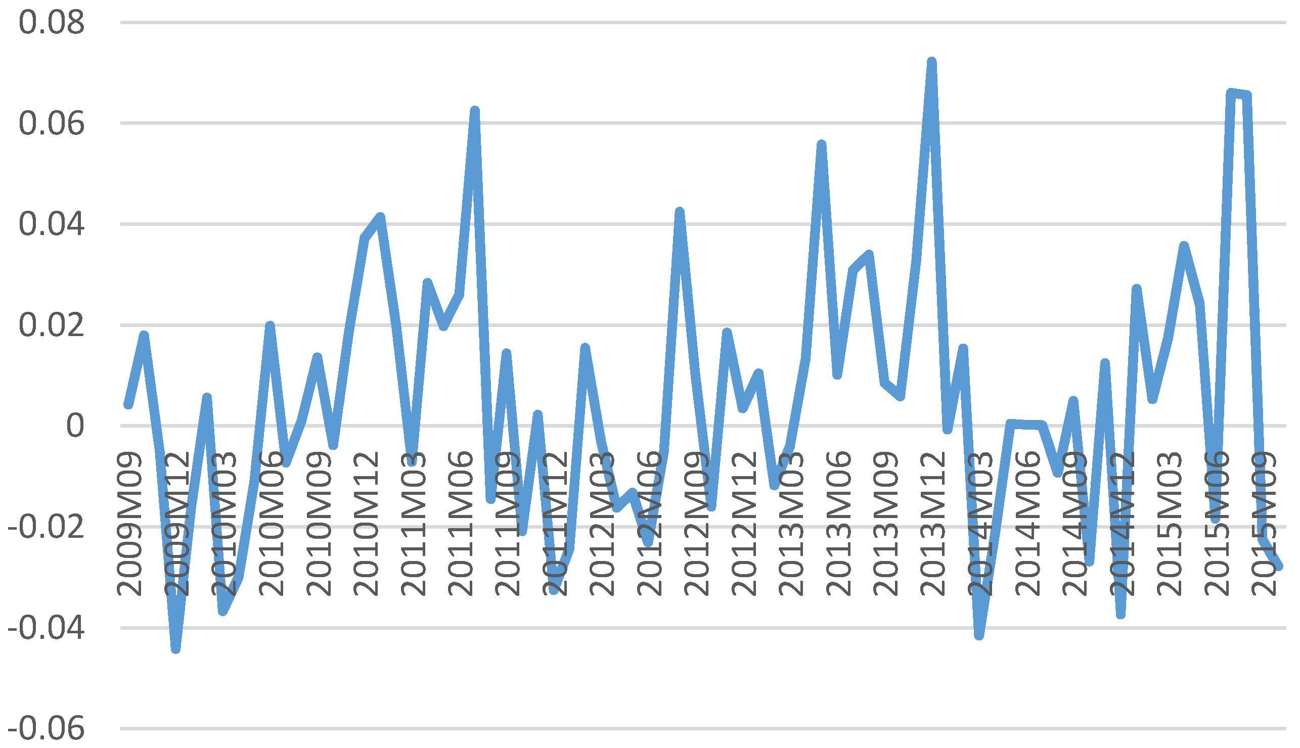
The global financial crisis, European debt crisis as well as changes in monetary policies of developed economies and country/region specific political instabilities have led to volatility in the value of currencies of emerging market economies. Particularly, in the Turkish economy, like many other emerging market economies, the volatility in national currency has increased in recent years. The Turkish Lira and Brazilian Real have depreciated the most among fragile quintet currencies. Figure 1 shows the volatility in the value of Turkish Lira against the Euro. Figure 1 shows that the volatility is quite high during the period after the global financial crisis took place in 2008 in the USA compared to the pre-crisis period. The nominal exchange rate increased by 56% from September 2009 to September 2015. The value of the national currency against the Euro has a crucial role in trade between Turkey and the Eurozone.
In 2014, European Union countries account for 43.5% of total export volume of Turkey while they account for 36% of import volume. In total trade, the European Union represents 40% of total foreign trade in the Turkish economy, valued at 157 billion US dollars. In this regard, any change in the value of each currency would affect the production sector of the Turkish economy [21] (p. 126).
In the pre-crisis period, risk appetite was high and global investors invested in high-risk and high-yield funds in emerging markets [22] (p. 42). However, the risk appetite has changed since the financial crisis. Investors now seek low-risk investments, even if they have low-yield. So, the risk appetite of global investors is low. Therefore, it is assumed they are more risk sensitive. In this respect, any change in financial system risk may have a greater impact on economic variables such as volatility in the value of national currencies, as explained before.
On the other hand, the response of an investor to a positive change in country risk may not be the same as with a negative shock. Investors would be diffident and skeptical when the risk gets lower and investors react slowly to new conditions. In this case, the mechanism may not work efficiently and national currency would appreciate only in the longer term. In the case of an increase in risk, investors would react swiftly and national currency would depreciate greatly in a very short period. Another issue concerning the risk appetite of investors is business cycles. Investors would search for safe heavens and would be more sensitive to risk factors. However, in the expansion periods, investors would become more willing to invest and the risk appetite would be high. In short, accuracy of the mechanism explaining the interaction between CDS spread and exchange rate is related to business cycles.
In this study, we aim to analyze the Turkish economy to understand the interaction between financial risk and exchange rate volatility in order to investigate how changes in financial risk affect national currency, in the cases of different shock types and during different stages of the business cycle. To measure the risk of financial systems, we employ CDS spreads as shown by [23]. We use an asymmetric causality test developed by [24] to observe the effects of positive and negative shocks separately and employ the MS VAR method in order to examine the interaction between variables under the different regimes. By doing so, we will be able to better understand the behavior of the EUR/TL exchange rate during type of shocks and in each stage of the business cycle. Also, we employ a frequency domain approach developed by [25] to investigate the causation linkage between risk factor and exchange rate in different time frequencies and the rolling windows causality test methods developed by [26] in order to see the exact dates where the causality between exchange rate and CDS occurs.
The Turkish economy suffers from exchange rate volatility because of its high foreign trade dependent structure that has prevailed since the 1980s. The share of European economies in Turkish foreign trade increases the Euro/Turkish Lira exchange rate value. In this regard, although there is a vast number of studies investigating determinants of exchange rate volatility, to our knowledge, there is no study investigating the relationship between CDS spreads and Euro/TL nominal exchange rate.
In the following section, we discuss the related findings in the literature. In the third section, we describe our economic methods. In the fourth section, we define our data used in the study. In the fifth section, we present empirical results obtained from MS-VAR and causality tests. Finally, we interpret our empirical findings and conclude our study.

2. Literature Review

The CDS market has grown over the last decade and, thus, has become more prominent in finance literature [27] (p. 271). Recent studies related to the CDS market have more focused on the determinants of CDS spreads. Authors use plenty of economic variables as a proxy to explain change in CDS spreads in different time periods.
In recent studies, exchange rate is employed as a proxy to investigate the factors inducing volatility in CDS spreads. It is accepted that exchange rate is one of the determinants of CDS spreads in a number of studies. Ehlers et al. [28], Duffie [29], Singh [30] and Kim et al. [31] include exchange rate in the model they build.
On the other hand, a group of studies analyze possible effects of CDS spreads on exchange rates to understand the linkage between credit risk of an economy and the strength of its currency, focusing on the post global crisis period due to depreciation in the US dollar as well as the Eurozone crisis. One of the initial studies investigating the effects of CDS on exchange rate belongs to [32]. They test the interaction between CDS spread and expectations in currency option market for the Mexican and Brazilian national currencies against the US dollar from 2005 to 2007. They suggest that the currency option market has consistently set prices considering the probability of a currency crash triggered by a corresponding sovereign default of Brazil and Mexico. Zhang et al. [13] take four developed economies into consideration to see possible interactions between national currencies and financial risk perceptions in terms of CDS spreads. They conclude that, in the pre-crisis period between January 2004 and February 2008, CDS spreads are leading indicators of the national currencies of Japan, United Kingdom of England, Australia and Eurozone vs. the US dollar.
Hui and Chung [17] studied 16 Eurozone countries in order to find a way to stabilize the Euro against the US dollar. They conclude that creditworthiness of not only countries with weaker fiscal conditions, but also those with strong fiscal positions may affect the market expectations of the stability of the Euro. Bekkour et al. [20] also pay attention to the Euro after the European Debt Crisis and analyzed the 2007–2012 period according to two sub-periods: the pre-crisis period from 2007 to 2009 and the post-crisis period from 2010 to 2012. Results of the research indicate that five-year CDS spreads of 11 European countries had an impact on common currency only during the sovereign debt crisis.
Omachel and Rudolf [33] investigate whether there is a direct relationship between sovereign defaults and exchange rate risks. Analysis results for nine European countries tell us that a CDS jump in a member country would induce depreciation in the Euro vs. US dollar. Another study looking at the Eurozone belongs to [18]. Different from other studies, Hui and Fong [18] tries to answer the question of how CDS spreads affect the currency of economies known as safe heavens, such as USA., Japan, Switzerland and Eurozone. In this regard, they analyze the long and short term interaction between CDS spread differentials, currency options and other macroeconomic variables. Results show that relative sovereign credit risk of these developed economies impacts the market expectations of their exchange rates in the long run, but not in the short run. Also, they report that the extent of the impact changes drastically in times of crisis.
A broader country analysis was conducted by Della Corte et al. [34]. They include 20 developed and developing countries into a panel data test. They find a linkage between sovereign risk and currency option as well as spot exchange rate between the years 2003 and 2013. Increasing sovereign risk shows a significant depreciation as well as higher volatility on exchange rate and it is mostly driven by countries’ exposures to global sovereign risk, whereas purely local sovereign risk matters much less.

3. Methodology

In this study, we employ a number of advanced causality analysis methods. The asymmetric causality test developed by Hatemi-J and Roca [24] allows us to investigate the asymmetrical causation linkage in different shock types, the frequency domain causality test developed by [25] allows us to find causality in different time frequencies, and the rolling windows causality test developed by [26] investigates the exact dates which causation linkages appear. The reason why we employ numerous causality methods is to investigate the causality from different perspectives. Although these causality analyses are based on a vector autoregressive method, they have different statistical strengths. The asymmetric causality and rolling windows causality are known as time domain causality analyses, while Breitung and Candelon’s analysis is based on frequency domain. By employing each method in the same model, we have the chance to test possible relationships from different perspectives. Lastly, we employ MS-VAR analysis in order to find responses of variables in different regimes. MS-VAR analysis method gives us the opportunity to break up the whole period into sub-periods delineating different business cycles, such as contraction and expansion.

3.1. Hatemi-J and Roca (2014) [24] Asymmetric Causality Test

P 1 t and P 2 t is two co-integrated variables [24] (p. 7)
P 1 t = P 1 t 1 + ε 1 t = P 1 , 0 + i = 1 t ε 1 i
and
P 2 t = P 2 t 1 + ε 2 t = P 2 , 0 + i = 1 t ε 2 i
t is t = 1, 2, …, T, P 1 , 0 and P 2 , 0 constant terms, ε 1 i , ε 2 i i i d ( 0 , δ 2 ) . Positive and negative changes in each variables are ε 1 i + = max ( ε 1 i , 0 ) , ε 2 i + = max ( ε 2 i , 0 ) , ε 1 i = min ( ε 1 i , 0 ) and ε 2 i = min ( ε 2 i , 0 ) , respectively. We estimate results as ε 1 i = ε 1 i + + ε 1 i and ε 2 i = ε 2 i + + ε 2 i , so,
P 1 t = P 1 t 1 + ε 1 t = P 1 , 0 + i = 1 t ε 1 i + + i = 1 t ε 1 i
P 2 t = P 2 t 1 + ε 2 t = P 2 , 0 + i = 1 t ε 2 i + + i = 1 t ε 2 i
The accumulation of positive and negative shocks in each variable are P 1 t + = i = 1 t ε 1 t + , P 1 t = i = 1 t ε 1 t , P 2 t + = i = 1 t ε 2 t + and P 2 t = i = 1 t ε 2 t , respectively [24] (p. 8). P t + = ( P 1 t + , P 2 t + ) vector is used in order to test causation linkage between positive shocks. For detailed information, we suggest to see [24] for bootstrap process and [35,36,37] for lag length selection.

3.2. Frequency Domain Causality Test

While conventional time domain causality tests produce a single test statistics for the interaction between variables of concern, the frequency domain methodology generates tests statistics at different frequencies across spectra. Frequency domain approach to causality thereby allows investigating causality dynamics at different frequencies rather than relying on a single statistic as is the case with the conventional time domain analysis [38]. Hence, it seems to be very meaningful to carry out frequency domain causality to better understand temporary and permanent linkages between policy rate and credit rates. To test for causality based on frequency domain, Geweke [39] and Hosoya [40] defined two-dimensional vector of time series z t = [ x t , y t ] and z t has a finite-order VAR
Θ ( L ) z t = ε t
where Θ ( L ) = I Θ 1 L Θ p L p and lag polynomial with L k z t = z t 1 . Then Granger causality at different frequencies is defined as
M y x = log [ 2 π f x ( ω ) | ψ 11 ( e i ω ) | 2 ] = [ 1 + | ψ 12 ( e i ω ) | 2 | ψ 11 ( e i ω ) | 2 ]
If | ψ 12 ( e i ω ) | 2 = 0 that y does not cause x at frequency ω . If components of z t are I(1) and co-integrated, then the autoregressive polynomial Θ ( L ) has a unit root. The remaining roots are outside the unit circle. Extracting z t 1 from both sides of Equation (7) gives
Δ z t = ( Θ 1 I ) z t 1 + Θ 1 z t 2 + + Θ p z t p + ε t = Θ ^ ( L ) z t 1 + ε t
where Θ ^ ( L ) = Θ 1 I + Θ 2 L + + Θ p L p [25]. Geweke [39] and Hosoya [40] propose causality measure at a particular frequency based on a decomposition of the spectral density. Breitung and Candelon [25], using a bivariate vector autoregressive model, propose a simple test procedure that is based on a set of linear hypothesis on the autoregressive parameters. So, the test procedure can be generalized to allow for co-integration relationships and higher-dimensional systems. For detailed information about the procedure, please see [25].

3.3. Balcilar et al. (2010) [26] Bootstrap Rolling Window Causality Test

Breitung and Candelon [26] run a LR (likelihood ratio) causality test using bootstrap method depending on error term. LR Granger causality test depending on bootsrap has two variables VAR (p) in the model, t = 1, 2, …, T;
y t = Φ 0 + Φ 1 y t 1 + + Φ p y t p + ε t
In the equity above, ε t = ( ε 1 , ε 2 ) i i d ( 0 , σ 2 ) is a covariance matrix Σ that is not odd. Optimal lag length criteria is defined by Akaike Information Criteria (AIC). While y t = [ y 1 t , y 2 t ] 2 x 1 considered as matrix, VAR (p) model will be shown as;
[ y 1 t y 2 t ] = [ ϕ 10 ϕ 20 ] + [ ϕ 11 ( L ) ϕ 12 ( L ) ϕ 21 ( L ) ϕ 22 ( L ) ] [ y 1 t y 2 t ] + [ ε 1 t ε 2 t ]
when ϕ i j ( L ) = k = 1 p ϕ i j , k L k , i, j = 1, 2, …, k lag operator, L k x t = x t k . Null hypothesis of the test is; where ϕ 12 , i = 0 , y 2 t is not Granger cause of y 1 t , or oppositely, where ϕ 21 , i = 0 , y 1 t is not Granger cause of y 2 t . In order to avoid possible structural unit roots and to get over the problems those are related to the size of the sample, Balcilar et al. [26] use the bootstrap test that is modified by [41,42] rolling window Granger causality test. For further details please see [26].

3.4. Markov Switching VAR Methodology

As an empirical methodology, Markov Switching Vector Autoregressive Model (MS-VAR) is applied on estimation of interaction between variables. The financial sector is quite sensitive to fluctuations in the economy and the crises would affect both CDS premium and the value of the national currency against foreign currencies. Hence, MS-VAR is a good tool for monitoring the asymmetric behaviors in the historical process and it has the advantage that one can accommodate structural changes across regimes, both with respect to autoregressive dynamics and the covariance structure of shocks [43].
The model examines behaviors of the time series in different regimes. The switching mechanism is controlled by an unobservable random variable. In these models, at any point of time during it is not possible to know which regime is effective. However, the observation probability of only one regime can be found at that time. MS-VAR model was originally developed by [44] and used by [44,45,46,47,48,49,50,51,52] for the empirical analysis of business cycle. According to [44], 2-regime MS-AR (p) model is established by following form
y t = { ϕ 1 , 0 + ϕ 1 , 1 y t 1 + + ϕ 1 , p y t p + ε t if ( s t = 1 ) ϕ 2 , 0 + ϕ 2 , 1 y t 1 + + ϕ 2 , p y t p + ε t if ( s t = 2 ) }
y t = ϕ 0 , s t + ϕ 1 , s t y t 1 + + ϕ p , s t y t p + ε t
where ϕ 1 , j and ϕ 2 , j denote autoregressive lag parameters for every regime, s t is the value of each regime, p shows degree of autoregressive process and ε i t is a sequence of independent and identically distributed random variables with mean zero and ε i t i i d ( 0 , σ i 2 ) and σ i 2 < [53,54,55]. Regimes are determined by an unobservable regime variable which is consistent with the Markov regime switching model. Regime varies depending on past value and transformation probabilities and it can be written by the following form
Pr ( S t = j | S t 1 = i ) = P i j 0
i , j = 1 , 2 , , k there are k different probable regimes and shows transition probabilities from regime i to regime j. This can be
j = 1 k Pr ( S t = j | S t 1 = i ) = 1
the transition of regime variable between regimes is controlled with Markov model. This model is expressed as follows
P [ a < y t b | y 1 , y 2 , , y t 1 ] = P [ a < y t b | y t 1 ]
If a variable removed Markov model, we have to calculate current period which will be within the next period regime and transformation probabilities [46] (p. 679) and [56] (p. 9)
P = ( P 11 P 1 k P k 1 P k k )
For example, if the probability of every regime is determined by vector π t = ( P 1 , P 2 , , P k ) in t time, so the probability of the every regime is determined by π t + 1 = P π t in t + 1 time. There is a ergodic probability vector, such as π = P π , for a stable Markov regime switching model. Ergodic probability vector can be considered as the unconditional probability of each regime. M-dimensional time series vector is defined as a conditional on y t = ( y 1 t , , y m t ) , s t { 1 , , k } [44]
P ( y t | Y t 1 , X t , s t ) = ( f ( y t | Y t 1 , X t , θ 1 ) if s t = 1 f ( y t | Y t 1 , X t , θ m ) if s t = k )
where P ( y t | Y t 1 , X t , s t ) is the probability density function of the vector of endogenous variables y t = ( y 1 t , , y m t ) which is conditional on the past behavior of the process, Y t 1 = { y t i } exogenous variables X t = { x t i } . The terms s t and θ m represent, respectively, regime variable and parameter vector when the series is in regime k [56] (p. 7). The model is assumed to be linear in each regime s t = k . In this context, if we consider white noise model as the autoregressive model and development models, ε i t i i d ( 0 , σ i 2 )
y t = n k + a k 1 y t 1 + + a k p y t p + ε t
Models represent a soft transition following regime shifts of time series. On the contrary, there is a leap at the first and last time point, when the time series shifted to the conditional mean in model [57] (pp. 374–376)
y t m ( s t ) = A 1 ( s t ) ( y t 1 m ( s t 1 ) ) + + A p ( s t ) ( y t p m ( s t p ) ) + u t
If stochastic model of y t is defined as conditional on unobservable regime s t , a full description of the data generating mechanism aims to specify stochastic model which occurs in the regime [58] and [55] (p. 201)
Pr ( s t | Y t 1 , S t 1 , X t , ρ )
where S t 1 = { s t j } j = 1 represents the history of the regime variable and it is not possible to observe its past but it might be found from observations and r is a vector of parameters of the regime generating process. In general, the regime variable cannot be observed and the historical behavior of the series must be obtained from the actual behavior of the process. Unobservable regime variable which is generated by ergodic Markov chain explains transformation probabilities and it is defined by the following form, p i j = 1 and i , j { 1 , , k } [54] (pp. 7–8).
p i j = Pr ( s t + 1 = j | s t = i )

4. Data Description

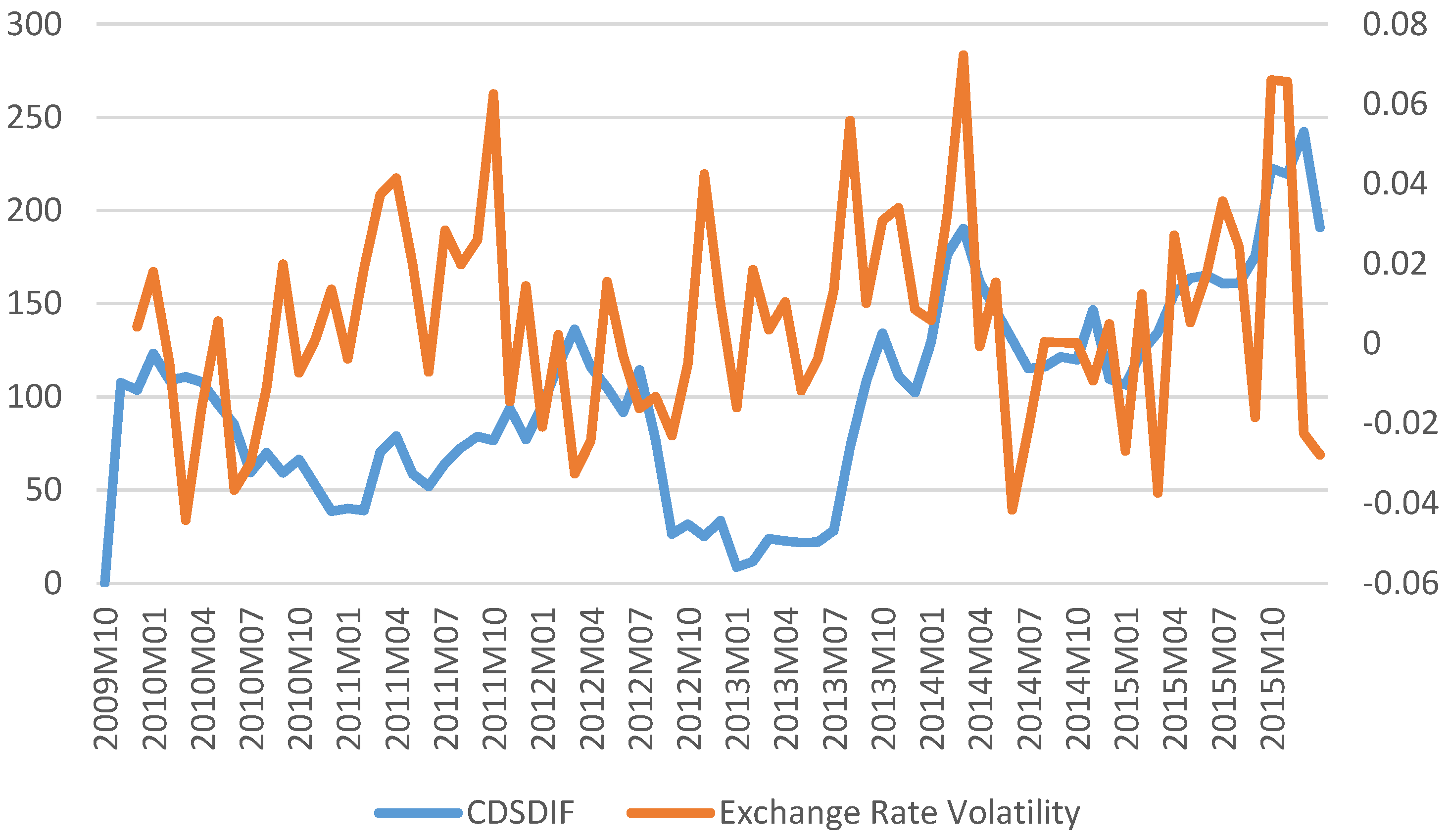
Before describing the data and its sources, it might be useful to show the movement of relative CDS spread of the Turkish economy and the volatility in the Turkish Lira. As can be seen in Figure 2, the EUR/TL exchange rate is volatile during the whole period. On the other hand, CDS spread has an increasing trend. It is worthy to mention that the CDS premium decreases in 2012 and an upward trend starts in 2013 again.
For the purpose of comparison, we use the perspectives of EURO-based investors in the analysis. We obtain monthly data belonging to five-year sovereign CDS spreads of the Eurozone calculated as a single premium for the whole area and Turkey from September 2009 to October 2015. Although there are numerous CDS premiums in different maturities, it is common to use CDS with five-year maturities to reflect risk in the related literature [17,18,19,20]. As exchange rate reflects the rate of exchange between two economies’ currencies, CDS spreads are thus expressed as the differences between the CDS spreads of the Turkish and Eurozone economies (the CDS spread of the Turkish economy minus the CDS spread of the Eurozone) (hereafter, CDS differential). We use monthly Euro/Turkish Lira nominal exchange rate data to measure the value of the Turkish Lira and five-year sovereign CDS spreads for each economy.
According to [23], CDS spreads are related to investors’ risk appetite associated with global event risk, financial market volatility and macroeconomic policy [59] (p. 184). Therefore, it is important to identify whether the sovereign CDS spreads and risk reversals of the Eurozone and Turkish economies in this study remain co-integrated in the presence of other macro-financial factors. In order to solve this problem, we include a set of macro-financial variables as control variables. These are macro-financial condition variables (Eurotraxx 50 and BIST 100 indexes), interest rate differential, historical inflation rate differential and global risk appetite (VIX index).
The Eurozone stock market index as proxy for the Eurotraxx 50 is used as a macroeconomic control variable. Similarly, the Turkish stock market index as proxy for the BIST 100 is employed as a control variable. To account for unusual turbulence in the stock market following the implosion of the Eurozone subprime market, we include the implied volatility of the Eurotraxx 50 index option (VIX) as an additional explanatory variable [13] (p. 448). Interest rate differential data (policy interest rate of the Turkish economy minus the Eurozone policy interest rate) is used as a control variable in order to see the effects of a possible increase in the interest rate differential on CDS spreads. Similarly, we add inflation rate differential data (Inflation rate in the Turkish economy minus inflation rate in the Eurozone economy) as another control variable into model.
As regards the data employed in this study, the monthly data belonging to 5-year CDS spreads for the Turkish and Eurozone economy, BIST 100 index, Eurotraxx 50 index, VIX index and EUR/TL nominal exchange rate are collected from Bloomberg database. Policy interest rate and inflation rate data for both economies are obtained from International Financial Statistics published by International Monetary Fund.
Table 1 shows descriptive statistics of variables in the model. Results indicate that volatility in CDS differential and interest rate differential variables are considerably high compared to other variables. Skewness coefficients show that the interest rate differential, inflation rate differential and BIST 100 index are skewed to the left and the others are skewed to the right. Kurtosis parameters imply the inflation differential and VIX series are steep, while the others are flattened compared to the inflation differential and VIX series. Results of Jarque-Bera test show only the inflation differential and VIX series are normally distributed.

5. Empirical Results

One important issue to be considered in an MS VAR analysis is testing stationary of variables. With this aim, we employ unit root test developed by [60,61] (Hereafter, ADF) and [62] (Hereafter, PP). According to results, BIST 100 index (BIST100, hereafter), Eurotraxx 50 index (EURTRX, hereafter), nominal exchange rate data (NEER, hereafter), CDS spreads differential (CDSDIF, hereafter), interest rate differential (INTDIF, hereafter) and inflation rate differential (INFDIF, hereafter) include the unit root in level and the first differential of the variables are stationary. So, the first differential of each variable must be used in the analysis.
According to Dickey-Fuller [61] and Phillips-Perron [62] test results in Table 2, variables are not stationary in level except the VIX variable. It is stationary at the 5% and 10% significance levels. However, we employ the first level of VIX variable because we assume it has long memory. When we employ the first differential of each variable, it is possible to conclude that there is no unit root and they are stationary in first difference. Moreover, we include trend and seasonality as external dummies in the model to get more robust results.
VAR (4) model in order to test Granger type causality is as follows
I n ( C D S D I F ) t = α 10 + i = 1 p α 11 i I n ( C D S D I F ) t i + i = 1 p α 12 i I n ( N E E R ) t i + i = 1 p α 13 i I n ( I N T D I F ) t i + i = 1 p α 14 i I n ( I N F D I F ) t i + i = 1 p α 15 i I n ( B I S T 100 ) t i + i = 1 p α 16 i I n ( V I X ) t i + i = 1 p α 17 i I n ( E U R S T X ) t i + ε 1 t
I n ( N E E R ) t = α 20 + i = 1 p α 21 i I n ( N E E R ) t i + i = 1 p α 22 i I n ( C D S D I F ) t i + i = 1 p α 23 i I n ( I N T D I F ) t i + i = 1 p α 24 i I n ( I N F D I F ) t i + i = 1 p α 25 i I n ( B I S T 100 ) t i + i = 1 p α 26 i I n ( V I X ) t i + i = 1 p α 27 i I n ( E U R S T X ) t i + ε 2 t
P is optimal lag length obtained from VAR model, ε t is an error correction parameter according to white noise hypothesis. In Equation (21), null hypothesis is α 12 i = 0 for ik and, in the case of accepting alternative hypothesis, it is accepted that there is a causality running from exchange rate to CDS differential. In Equation (22), null hypothesis is α 22 i = 0 for ik and, in the case of accepting the alternative hypothesis, it is accepted that there is a causality running from CDS differential to exchange rate.
According to results obtained from Hatemi-J and Roca [24] asymmetric causality test results in Table 3, a positive shock in CDS differential does not affect exchange rate positively or negatively. However, a negative shock in CDS differential that means a decrease in CDS premium of Turkey relative to Eurozone’s, would affect exchange rate negatively and positively. It means that a relative improvement in CDS premium of Turkey would induce an appreciation in the Turkish Lira. However, the result is statistically significant at the 10% level. Moreover, a negative shock in CDS differential—that means a decrease in CDS premium of Turkey relative to Eurozone’s—would affect nominal exchange rate positively, but the significance is only 5%.
Asymmetric causality test results also imply that an increase in exchange rate would affect CDS differential between Eurozone and Turkey. On the other hand, a decrease in exchange rate does not affect CDS differential, neither positively nor negatively. That means exchange rate is a determinant of CDS premium in the case of depreciation only and behaves asymmetrically.
According to results presented in Table 4 and obtained from the frequency domain causality test, there is a bi-directional causality between CDS differential and exchange rate in the long term. In the short run, the causality runs from nominal exchange rate to CDS differential. The results imply that we can classify nominal exchange rate as a determinant of CDS spread in the Turkish economy. Moreover, a change in CDS differential would induce volatility in the exchange rate in the long run. On the other hand, there is no causality running from CDS differential to exchange rate.
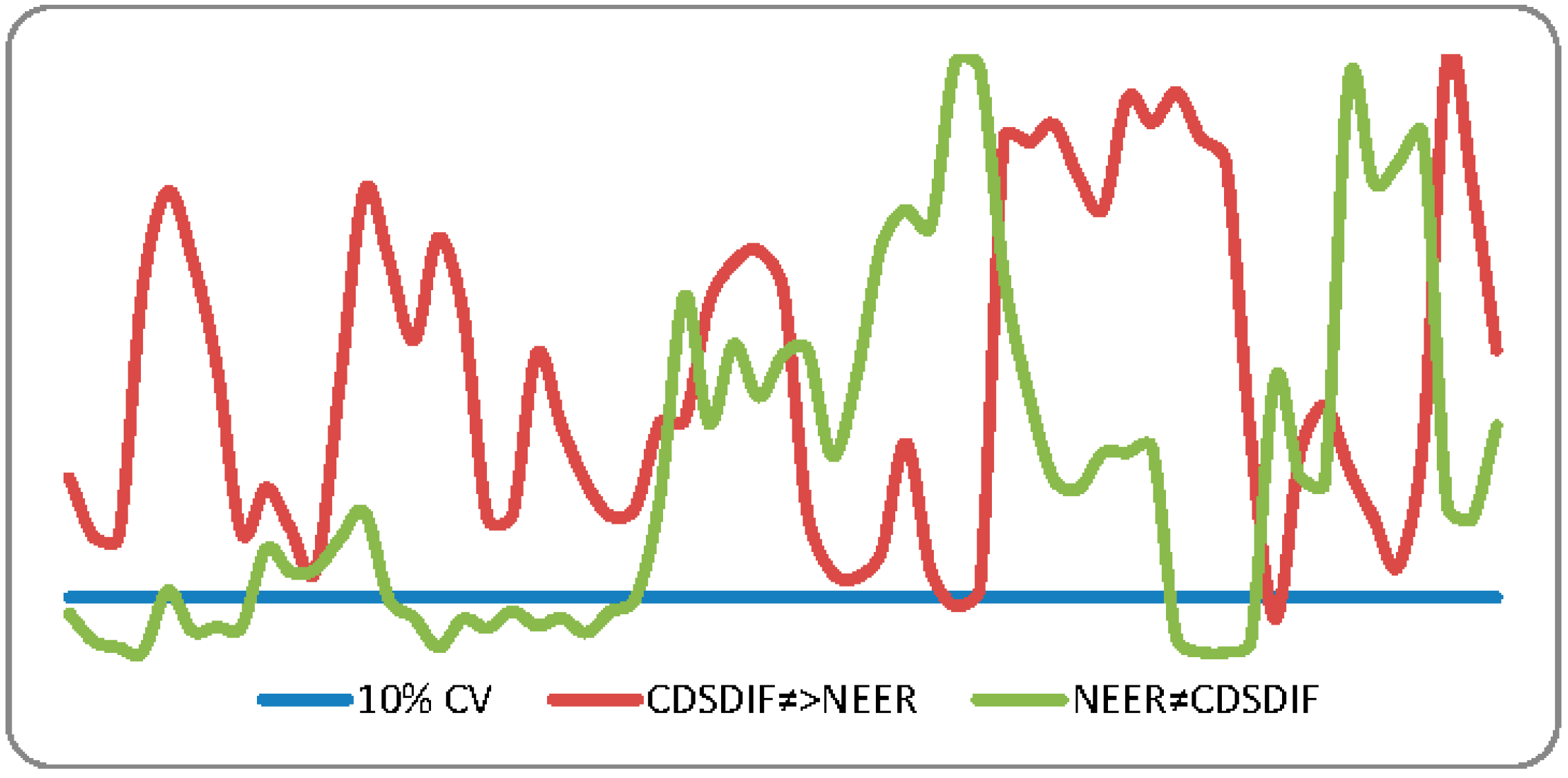
The rolling windows causality analysis results are presented in Figure 3. According to results, the causality running from CDS differential to nominal exchange rate occurs only in December 2013 and January 2015. On the other hand, the causation linkage from nominal exchange rate to CDS differential occurs in December 2010, January, Frebruary, March and April of 2011, for the full year of 2012, September, October, November and December of 2014.
According to the rolling windows causality test results, it is possible to say that CDS differential is not the main driver of nominal Eur/TL exchange rate in Turkey. The test results imply the causation linkage exists for only two months. The increasing fragility of the economies after the decleration of the Federal Reserve of United States may be the reason of existence of uni-directional causality in December 2013 and January 2015. On the other hand, results of both the frequency domain and rolling windows causality tests indicate the exchange rate is a determinant of CDS differential in the Turkish economy.
The first step of MS-VAR analysis is to determine number of regimes. In Table 5, LR (rate of probability) and Davies1 test statistics show that all regimes have a non-linear and asymmetric structure. According to test statistics, the model with two regimes has the smallest SC and AIC statistics, and besides it has the greatest rate of LR. The optimal lag length is determined to be 3 according to AIC and HQ information criteria. In light of this finding, we build the model as MSIA(3)–VAR(2). We also employ this model to obtain transition probability matrices presented in Table 6.
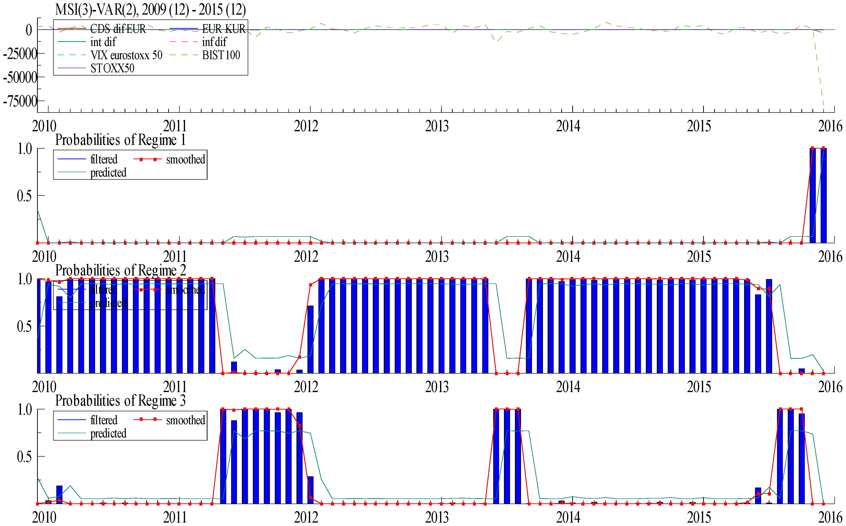
According to regime transition probability results presented in Table 6, while economy is in the first regime, the probability of it remaining in the same regime is 47% and the probability of a transition to the second regime is 25% and to the third regime is 14%. On the other hand, if the economy is in the second regime, the probability of it remaining in the same regime is 73%, while the probability of a transition to the first regime is 13% and a transition to regime 3 is 12%. If the economy is in the third regime, the probability of it remaining in the same regime is 64% and the probabilities of a transition to other regimes are 10% and 24%, respectively. According to regime analysis results, the length of regime one is 0.96 years while it is 1.09 years for the second period. The speed of entrance to the second regime is 0.32 years and speed of entrance to the first regime is 0.33 years. Graphical analysis of transition movement of variables among regimes is presented in Figure 4.
In total, 19.45% of observations belong to regime one, 53% of belongs to regime 2 and 27% of the observations belong to regime three. The lengths of regimes are 1.89, 3.76 and 2.82 years, respectively.
The impulse-response analysis results belonging to first regime is presented in the Table 7. According to results, 1% positive shock in CDS differential would induce a positive shock in exchange rate. However, in the second month, the response is negative. This result means that it is statistically insignificant. On the other hand, the response of exchange rate to a positive shock in interest rate differentials is positive and significant. It means that an increase in interest rates in Turkey or a decrease in the Eurozone would depreciate the exchange rate. Despite being statistically significant theoretically, it appears insignificant. An increase in the inflation rate differential would depreciate the exchange rate. The result is significant both statistically and theoretically. A positive shock in the VIX variable, which indicates the risk perception in the Eurozone stock market, would appreciate the nominal exchange rate. This result also be significant both theoretically and statistically. A positive shock in BIST 100 index would induce an increase in the nominal exchange rate but it is statistically insignificant. On the other hand, a positive shock in Eurostoxx 50 index would depreciate the nominal exchange rate. The result is significant statistically and theoretically.
The impulse-response analysis results belonging to second regime are presented in Table 8. According to results, the response of exchange rate to a positive shock in CDS differential is positive and statistically significant for 10 months at least. The exchange rate decreases in the following months. Similarly, response of exchange rate to a positive shock in inflation rate differential is positive and significant statistically and theoretically. Conversely, the response of the exchange rate to a positive shock in the interest rate differential is negative. It is significant for two months. It is theoretically significant because an increase in interest rates would appreciate the nominal exchange rate due to capital inflows. On the other hand, an increase in risk perception in the European stock market would appreciate the nominal exchange rate significantly for the whole period. The responses of the nominal exchange rate to positive shocks in BIST 100 and Eurostoxx 50 indexes are statistically insignificant.
The impulse-response analysis results belonging to the third regime are presented in the Table 9. According to results, the response of exchange rate to a positive shock in CDS differential is negative and statistically significant for three months. However, it is insignificant theoretically. Similarly, a response of exchange rate to a positive shock in the inflation rate differential is positive and insignificant statistically and theoretically. The response of exchange rate to a positive shock in interest rate differential is positive and, although it is significant statistically, it is insignificant theoretically. On the other hand, an increase in risk perception in the European stock market would depreciate nominal exchange rate significantly for a quarter. The response of the nominal exchange rate to positive shocks in BIST 100 index is statistically insignificant. The response of nominal exchange rate to a shock in Eurostoxx 50 index is statistically significant but theoretically insignificant.

6. Conclusions

This study determines the nature of the causal relationship between CDS spreads and the nominal EUR/TL exchange rate in the Turkish economy. A novel approach to Markov Switching VAR method, which investigates the relationship in multiple periods is applied to the Turkish economy during the period 2009–2015. Furthermore, we also carry out asymmetric, frequency domain and rolling windows causality analyses, which have different statistical strengths. They are useful for determining exact dates causality occurs and for investigating the causation linkage in the case of asymmetric shocks and in different time frequencies. So, we are able to analyze the model from different perspectives.
The results obtained from asymmetric causality analysis show that a decrease in CDS would appreciate the EUR/TL exchange rate while an increase in CDS would not depreciate. Similarly, frequency domain causality analysis results imply the existence of a causation linkage between CDS and nominal exchange rate in the long run. The rolling windows causality analysis results emphasize that the causal relationship from CDS spreads to EUR/TL exchange rate only in 2013 and 2015.
The MS VAR analysis results show that the Turkish economy experiences three regimes in the period between years 2009 and 2015. Impulse-response analysis results show that the impact of CDS spreads on EUR/TL exchange rate is positive and significant in only the second regime. MS VAR analysis results imply that the interest rate differential and inflation rate differential between economies and risk perception of European investors affect EUR/TL nominal exchange rate significantly in the second regime only.
According to the results obtained from all econometric analysis methods, there is a causation linkage running from CDS spread to EUR/TL exchange rate. However, the strength of causality differs according to the regime and direction of shock. The results imply that observation of CDS spread changes might be useful in predicting exchange rate instability. This would assist policymakers in efforts to stabilize the value of the Turkish Lira against foreign currencies. Also, the results conclude that CDS spreads of each economy could be used as a direct measure of economic risk in exchange rate models. On the other hand, the nominal value of the Turkish Lira against the Euro is an important factor affecting CDS premiums.

Author Contributions

All authors contributed equally to the paper.

Conflicts of Interest

Authors declare no conflict of interest.

References

  1. R. Dornbusch. “Exchange Rate Economics: Where Do We Stand? ” Brookings Pap. Econ. Activity 11 (1980): 143–206. [Google Scholar] [CrossRef]
  2. W.H. Branson. “Macroeconomic Determinants of Real Exchange Rates.” NBER Working Paper No. 801. 1981. Available online: http://www.nber.org/papers/w0801 (accessed on 15 February 2016).
  3. R.S. Pindyck, and J.J. Rotemberg. “The excess co-movement of commodity prices.” Econ. J. 100 (1990): 1173–1189. [Google Scholar] [CrossRef]
  4. J.H. Bergstrand. “Structural determinants of real exchange rates and national price levels: Some empirical evidence.” Am. Econ. Rev. 81 (1991): 325–334. [Google Scholar]
  5. H. Faruqee. “Long-run determinants of the real exchange rate: A stock-flow perspective.” Int. Money Fund Staff Pap. 42 (1995): 80–107. [Google Scholar] [CrossRef]
  6. R. Clarida, and J. Gali. “Sources of real exchange rate fluctuations: How important are nominal shocks.” Carnegie Rochester Conf. Ser. Public Policy 41 (1994): 1–56. [Google Scholar] [CrossRef]
  7. N.C. Mark, and D.Y. Choi. “Real exchange rate prediction over long horizons.” J. Int. Econ. 43 (1997): 29–60. [Google Scholar] [CrossRef]
  8. M.D. Chinn. “Real Exchange Rates.” Available online: http://citeseerx.ist.psu.edu/viewdoc/download?doi=10.1.1.363.1561&rep=rep1&type=pdf (accessed on 15 February 2016).
  9. J. Zalduendo. “Determinants of Venezuela’s Equilibrium Real Exchange Rate.” IMF Working Paper. 2006. Available online: http://www.imf.org/external/pubs/ft/wp/2006/wp0674.pdf (accessed on 15 February 2016).
  10. S.S. Golub. “Oil prices and exchange rates.” Econ. J. 93 (1983): 576–593. [Google Scholar] [CrossRef]
  11. P. Krugman. “Oil and the dollar.” NBER Working Paper No. 554. 1980. Available online: http://www.nber.org/papers/w0554.pdf (accessed on 23 April 2015).
  12. S. Nazlioglu, T. Bayat, and S. Kayhan. “Exchange rate and oil price interactions in transition economies: Czech Republic, Hungary and Poland.” Panoeconomicus 62 (2015): 267–285. [Google Scholar]
  13. G. Zhang, Y. Jot, and H.G. Fung. “Do credit default swaps predict currency values? ” Appl. Financ. Econ. 20 (2010): 439–458. [Google Scholar] [CrossRef]
  14. B. Eichengreen, A.K. Rose, and C. Wyplosz. “Exchange market mayhem: The antecedents and aftermath of speculative attacks.” Econ. Policy 21 (1995): 249–312. [Google Scholar] [CrossRef]
  15. B. Eichengreen, and R. Hausmann. “Exchange Rates and Financial Fragility.” NBER Working Paper 7418. 1999. Available online: www.nber.org/papers/w7418.pdf (accessed on 10 February 2016).
  16. M. Obstfeld, and K. Rogoff. “The six major puzzles in international macroeco-nomics: Is there a common cause? ” 2000. Available online: www.nber.org/papers/w7777 (accessed 10 February 2016).
  17. C.H. Hui, and T.K. Chung. “Crash risk of the euro in the sovereign debt crisis of 2009–2010.” J. Bank. Financ. 35 (2011): 2945–2955. [Google Scholar] [CrossRef]
  18. C. Hui, and T.P. Fong. “Price cointegration between sovereign CDS and currency option markets in the financial crises of 2007–2013.” Int. Rev. Econ. Finance 40 (2015): 174–190. [Google Scholar] [CrossRef]
  19. L. Yang, B. Morley, and J. Hudson. “A study of the causal relationships between sovereign CDS spreads, risk-free interest rates and exchange rates.” In Proceedings of the 8th INFINITI Conference on International Finance, Dublin, Ireland, 14–15 May 2010.
  20. L. Bekkour, X. Jin, T. Lehnert, F. Rasmouki, and C. Wolff. “Euro at risk: The impact of member countries’ credit risk on the stability of the common currency.” J. Empir. Finance 33 (2015): 67–83. [Google Scholar] [CrossRef]
  21. TIM (Türkiye İhracatçılar Meclisi). Ekonomi ve dış ticaret raporu 2014. İstanbul, Turkey: Türkiye İhracatçılar Meclisi Yayını, 2015. [Google Scholar]
  22. G. Ozgur, and H. Ozel. “Kuresellesme, finansal genisleme ve bunalim.” Amme Idaresi Dergisi 43 (2010): 33–56. [Google Scholar]
  23. J. Pan, and K.J. Singleton. “Default and recovery implicit in the term structure of sovereign CDS spreads.” J. Finance 13 (2008): 2345–2385. [Google Scholar] [CrossRef]
  24. A. Hatemi-J, and E. Roca. “BRICs and PIGS in the presence of Uncle Sam and big brothers: Who drive who? Evidence based on asymmetric causality tests.” 2014. Available online: http://econpapers.repec.org/paper/griapaper/finance_3a201401.htm (accessed on 10 October 2015).
  25. J. Breitung, and B. Candelon. “Testing for short and long-run causality: A frequency domain approach.” J. Econom. 12 (2006): 363–378. [Google Scholar] [CrossRef]
  26. M. Balcilar, Z.A. Ozdemir, and Y. Arslanturk. “Economic growth and energy consumption causal nexus viewed through a bootstrap rolling window.” Energy Econ. 32 (2010): 1398–1410. [Google Scholar] [CrossRef]
  27. K. Galil, O.M. Shapir, D. Amiram, and U. Ben-Zion. “The determinants of CDS spreads.” J. Bank. Finance 41 (2014): 271–282. [Google Scholar] [CrossRef]
  28. P. Ehlers, and P. Schonbucher. “The influence of FX risk on credit spreads.” Available online: http://www.actuaries.org/afir/colloquia/zurich/ehlers_schoenburcher.pdf (accessed on 10 February 2016).
  29. D. Duffie. “Credit default valuation.” Financ. Anal. J. 55 (1999): 73–87. [Google Scholar] [CrossRef]
  30. M. Singh. A New Methodology to Proxy Recovery Value in CDS Contracts. IMF Working Paper No. 03/242; Washington, D.C., USA: IMF, 2003. [Google Scholar]
  31. T.S. Kim, Y.J. Park, and J. Park. “Macroeconomic conditions and credit default swap spread changes.” In Proceedings of the European Financial Management Association 2015 Annual Meetings, Amsterdam, The Netherlands, 24–27 June 2015.
  32. P. Carr, and L. Wu. “Theory and evidence on the dynamic interactions between sovereign credit default swaps and currency options.” J. Bank. Finance 31 (2007): 2383–2403. [Google Scholar] [CrossRef]
  33. M. Omachel, and M. Rudolf. “The Linkage between Sovereign Defaults and Exchange Rate Shocks in the Eurozone: A Measure for Systemic Risk.” 2015. Available online: http://ssrn.com/abstract=2513178 (accessed on 10 February 2016).
  34. P. Della Corte, L. Sarno, M. Schmeling, and C. Wagner. “Exchange Rates and Sovereign Risk.” 2015. Available online: http://ssrn.com/abstract=2354935 (accessed on 10 February 2016).
  35. A. Hatemi-J. “A new method to choose optimal lag order in stable and unstable VAR models.” Appl. Econ. Lett. 10 (2003): 135–137. [Google Scholar] [CrossRef]
  36. A. Hatemi-J. “Forecasting properties of a new method to choose optimal lag order in stable and unstable VAR models.” Appl. Econ. Lett. 15 (2008): 239–243. [Google Scholar] [CrossRef]
  37. H. Lütkepohl. New Introduction to Multiple Time Series Analysis. Berlin, Germany: Springer, 2005. [Google Scholar]
  38. C. Ciner. “Eurocurrency interest rate linkages: A frequency domain analysis.” Int. Rev. Econ. Finance 10 (2011): 498–505. [Google Scholar] [CrossRef]
  39. J. Geweke. “Measurement of linear dependence and feedback between multiple time series.” J. Am. Stat. Assoc. 77 (1982): 304–313. [Google Scholar] [CrossRef]
  40. Y. Hosoya. “The decomposition and measurement of the interdependence between second-order stationary process.” Probab. Theory Relat. Fields 88 (1991): 429–444. [Google Scholar] [CrossRef]
  41. A. Koutris, M.S. Heracleous, and A. Spanos. “Testing for nonstationarity using maximum entropy resampling: A misspecification testing perspective.” Econom. Rev. 27 (2008): 363–384. [Google Scholar] [CrossRef]
  42. G. Shukur, and P. Mantalos. “A simple investigation of the Granger-causality test in integrated-cointegrated VAR systems.” J. Appl. Stat. 27 (2000): 1021–1031. [Google Scholar] [CrossRef]
  43. M. Binder, and M. Gross. “Regime-switching global vector autoregressive models.” ECB Working Paper No. 1569. 2013. Available online: https://www.ecb.europa.eu/pub/pdf/scpwps/ecbwp1569.pdf?d2d0799b7984bf9aa815ed4192419033 (accessed on 20 April 2015).
  44. J.D. Hamilton. “A new approach to the economic analysis of nonstationary time series and the business cycle.” Econometrica 57 (1989): 357–384. [Google Scholar] [CrossRef]
  45. J.D. Hamilton. “Analysis of time series subject to regime changes.” J. Econom. 45 (1990): 39–70. [Google Scholar] [CrossRef]
  46. J.D. Hamilton. Time Series Analysis. Princeton, NJ, USA: Princeton University Press, 1994, Chapter 22. [Google Scholar]
  47. J.D. Hamilton. “Specification testing in Markov-switching time-series models.” J. Econom. 70 (1996): 127–157. [Google Scholar] [CrossRef]
  48. C.J. Kim, and G. Nelson. State-Space Models with Regime-Switching: Classical and Gibbs-Sampling Approaches with Applications. Cambridge, MA, USA: MIT Press, 1998. [Google Scholar]
  49. H.M. Krolzig. Markov Switching Vector Autoregressions. Modelling, Statistical Inference and Application to Business Cycle Analysis. Berlin, Germany: Springer, 1997. [Google Scholar]
  50. H.M. Krolzig. Econometric Modelling of Markov-Switching Vector Autoregressions Using MSVAR for Ox. New York, NY, USA: Oxford University Press, 1998. [Google Scholar]
  51. H.M. Krolzig. Predicting Markov-Switching Vector Autoregressive Processes. New York, NY, USA: Oxford University Press, 2000. [Google Scholar]
  52. H.M. Krolzig. Estimation, Structural Analysis and Forecasting of Regime-Switching Model with MSVAR for Ox. New York, NY, USA: Oxford University Press, 2001. [Google Scholar]
  53. T.I. Mohd, and I. Zahid. “Modelling exchange rates using regime switcing models.” Sains Malaysiana 35 (2006): 55–62. [Google Scholar]
  54. F. Fallahi, and G. Rodriguez. Using Markov-switching models to identify the link between unemployment and criminality. Working Paper. No #0701E, 1–53; Ottowa, Canada: Faculty of Social Sciences, University of Ottawa, 2007. [Google Scholar]
  55. S. Kayhan, T. Bayat, and A. Kocyigit. “Enflasyon hedeflemesi rejiminde ogrenme sureci ve asimetri: Markov switching yaklasimi.” Eskiseh. Osman. Univ. IIBF Dergisi 8 (2013): 191–212. [Google Scholar]
  56. S. Owen. “A Markov Switching Model for UK Acquisition Levels.” School of Banking and Finance, University of New South Wales, Working Paper No. 2004-1. 2004. Available online: http://wwwdocs.fce.unsw.edu.au/banking/workpap/wp%2001%202004.pdf (accessed on 15 June 2014).
  57. L. Ferrara. “A three-regime real-time indicator for the US economy.” Econ. Lett. 80 (2003): 373–378. [Google Scholar] [CrossRef]
  58. M. Bildirici, and U. Bozoklu. Bireysel Beklentiler ve Çoklu Ekonomik Denge: Markov Geçiş Modeli. 8. Malatya, Turkey: Türkiye Ekonometri ve İstatistik Kongresi, İnönü Üniversitesi, 2007, pp. 1–10. [Google Scholar]
  59. C.H. Hui, C.-F. Lo, and T. Fong. “A quasi-bounded model for Swiss Franc’s one-sided target zone during 2011–2015.” Available online: http://www.hkimr.org/uploads/publication/421/wp-no-15_2015-final-.pdf (accessed on 10 February 2016).
  60. D. Dickey, and W. Fuller. “Distribution of the estimators for autoregressive time series with a unit root.” J. Am. Stat. Assoc. 74 (1979): 427–431. [Google Scholar]
  61. D. Dickey, and W. Fuller. “Likelihood ratio statistics for autoregressive time series with a unit root.” Econometrica 49 (1981): 1057–1072. [Google Scholar] [CrossRef]
  62. P.C. Phillips, and P. Perron. “Testing for a unit root in time series regression.” Biometrika 75 (1988): 335–346. [Google Scholar] [CrossRef]
  63. J.G. MacKinnon. “Numerical distribution functions for unit root and co-integration tests.” J. Appl. Econom. 11 (1996): 601–618. [Google Scholar] [CrossRef]
  64. R.B. Davies. “Hypothesis testing when a nuisance parameter is present only under the alternative.” Biometrika 4 (1977): 247–254. [Google Scholar] [CrossRef]
  65. R.B. Davies. “Hypothesis testing when a nuisance parameter is present only under the alternative.” Biometrika 74 (1987): 33–43. [Google Scholar]
  66. R. Garcia, and P. Perron. “An analysis of the real interest rate under regime shifts.” Rev. Econ. Stat. 78 (1996): 111–125. [Google Scholar] [CrossRef]
  • 1For detailed information about Davies asymmetry test, please see Davies [64] and [65] and Garcia and Perron [66].
Figure 1. Volatility in the value of the Lira against the Euro (percentage change compared to previous month).
Ijfs 04 00014 g001
Figure 2. Volatility in nominal exchange rate (Right Axis) and Changes in CDS differential (Left Axis) (Volatility in nominal exchange rate calculated due to change compared to previous month, CDS differentials are in absolute value.).
Ijfs 04 00014 g002
Figure 3. Balcilar et al. [26] bootstrap rolling window causality results.
Ijfs 04 00014 g003
Figure 4. Smoothed avg. posterior probability of regimes 1, 2 and 3.
Ijfs 04 00014 g004
Table 1. Descriptive statistics of variables.
ETFsMeanMax.Min.Standard Dev.SkewnessKurtosisJarque-Bera (p-value)
CDSDIF100.16242.318.64753.6270.37192.78191.8778
NEER2.49473.38091.92730.37450.39652.16844.1270
INTDIF4.8227.850.002.2424−0.44022.40013.5478
INFDIF6.46449.28071.31091.8701−0.83393.27968.9368
BIST10068,442.990,094.546,533.511,182.7−0.05051.92763.6256
VIX23.87846.686.956.55340.69964.04919.5589
EURTRX2865.13697.42118.9377.240.22642.40731.7384
Table 2. ADF and PP unit root test results.
Levels-VariablesADFPPFirst DifferencesVariablesADFPP
ConstantBIST100−1.848 (0)
[0.354]
−1.898 (3)
[0.331]
BIST100−7.445 (0)
[0.00] ***
−7.393 (6)
[0.00] ***
CDSDIF−0.680 (0)
[0.844]
−0.728 (2)
[0.832]
CDSDIF−8.002 (0)
[0.00] ***
−7.927 (3)
[0.00] ***
NEER0.350 (0)
[0.979]
0.045 (3)
[0.959]
NEER−6.771 (0)
[0.00] ***
−6.771 (1)
[0.00] ***
INFDIF−2.186 (0)
[0.212]
−2.312 (1)
[0.170]
INFDIF−7.790 (0)
[0.00] ***
−7.789 (1)
[0.00] ***
INTDIF−1.400 (0)
[0.577]
−1.650 (3)
[0.452]
INTDIF−7.477 (0)
[0.00] ***
−7.470 (1)
[0.00] ***
EURTRX−1.133 (0)
[0.698]
−1.133 (0)
[0.698]
EURTRX−8.779 (0)
[0.00] ***
−8.819 (2)
[0.00] ***
VIX−3.019 (1)
[0.038] **
−5.057 (4)
[0.00] ***
VIX−14.695 (0)
[0.00] ***
−15.693 (3)
[0.00] ***
Constant + TrendBIST−2.352 (0)
[0.400]
−2.529 (1)
[0.313]
BIST−7.414 (0)
[0.00] ***
−7.357 (6)
[0.00] ***
CDSDIF−1.767 (0)
[0.710]
−1.730 (3)
[0.727]
CDSDIF−8.205 (0)
[0.00] ***
−8.191 (6)
[0.00] ***
NEER−1.980 (0)
[0.602]
−2.279 (3)
[0.439]
NEER−6.832 (0)
[0.00] ***
−6.833 (1)
[0.00] ***
INF DIF−2.445 (0)
[0.353]
−2.706 (2)
[0.237]
INF DIF−7.735 (0)
[0.00] ***
−7.734 (1)
[0.00] ***
INT DIF−2.278 (0)
[0.439]
−2.437 (3)
[0.357]
INT DIF−7.504 (0)
[0.00] ***
−7.499 (1)
[0.00] ***
EURTRX−2.202 (0)
[0.481]
−2.210 (1)
[0.476]
EURTRX−8.788 (0)
[0.00] ***
−8.832 (2)
[0.00] ***
VIX−3.357 (1)
[0.065] *
−5.820 (4)
[0.00] ***
VIX−14.593 (0)
[0.00] ***
−15.604 (3)
[0.00] ***
The figures in parenthesis denote the lag length selected by the Schwarz criterion. ***, **, and * denote statistical significance at the 1%, 5% and 10% level of significance, respectively. Values within the brackets shows the probability ratios. For the ADF test: The results of Dickey Fuller test in the case of zero lag length and lag length chosen due to SIC criteria. For the ADF test, the Mac Kinnon [63] critical values for with constant −3.485, −2.885 at the 1%, and 5% levels. The critical values for with constant and trend −4.035, −3.447 at the 1% and 5% levels, respectively. For the PP test: Values in the parenthesis show bandwidths obtained according to Newey-West using Bartlett Kernel criteria. For the PP test Mac Kinnon [63] critical values for with constant −3.483, −2.884 at the 1% and 5% levels. The critical values for with constant and trend −4.033, −3.446 at the 1% and 5% levels, respectively.
Table 3. Hatemi-J and Roca [24] asymmetric causality test results.
Direction of CausalityMwald1%5%10%Direction of CausalityMwald1%5%10%
(CDSDIF)+ ≠> (NEER)+0.052 (0.819)7.5254.4872.262(NEER)+ ≠> (CDSDIF)+3.782 (0.052) *9.0235.0643.319 *
(CDSDIF)+ ≠> (NEER)3.699 (0.157)12.1686.7934.922(NEER)+ ≠> (CDSDIF)11.058 (0.004) ***14.0748.048 **5.804 *
(CDSDIF) ≠> (NEER)3.224 (0.073) *8.4774.9023.318(NEER) ≠> (CDSDIF)0.210 (0.646)8.3814.2832.745
(CDSDIF) ≠> (NEER)+6.529 (0.038) **12.2517.0615.090 *(NEER) ≠> (CDSDIF)+3.284 (0.194)10.8176.5394.801
≠> shows null hypothesis where there is no causality. Values in parenthesis show asymptotic probability values. ***, ** and * show 1%, 5% and 10% significance levels, respectively. The number of bootstrap iterations is 10,000.
Table 4. Breitung and Candelon [26] frequency domain causality analysis results.
Direction of CausalityLong TermMedium TermShort Term
ωi0.010.051.001.502.02.50
CDSDIF ≠> NEER3.762 **3.817 **5.947 **0.3441.5742.744
NEER ≠> CDSDIF6.863 **6.819 **6.115 **9.898 **6.128 **0.553
Notes: Lag lengths for the VAR models are determined by SIC. F distribution with (2, T-2p) degrees of freedom equals about 3,15 for every ωi (frequency) between 0 and π. ω ∈ (0, π). ** denotes significance in 5 % level.
Table 5. Test statistics and regime determinants for VAR(2) Model.
No. of RegimeLog ProbLR LinearityDaviesAICSC
MS(2)−1724.8929239.31540.0053.832761.3630
MS(3)−1464.7980759.50520.0049.693160.6434
MS(4)−1782.8227123.45580.0053.392458.6008
AIC denotes Akaike Information Criteria, SC denotes Schwarz Information Criteria, LR denotes rate of probability.
Table 6. Regime transition probability matrices.
No. of RegimeNumber of ObservationsDurationRegime 1Regime 2Regime 3
Regime 114.21.900.47340.38030.1462
Regime 238.83.760.13710.73420.1287
Regime 320.02.830.10460.24910.6463
Table 7. Response of EXC to 1% positive shock in other variables in regime 1.
No. of PeriodsCDSEXCINTDIFINFDIFVIXBIST100EURSTX
10.27860.36600.72540.0368−0.44100.12070.3886
2−0.23240.13490.42300.2944−0.2058−0.70390.8148
3−0.17190.49700.16980.1742−0.8476−0.24010.3690
4−0.79180.18300.64940.7382−0.3256−0.10940.1088
5−0.31040.67380.24310.2886−0.1221−0.33340.4420
6−0.11880.24810.90090.1089−0.4531−0.12400.1509
7−0.44130.91330.33270.4054−0.1674−0.41040.5778
8−0.16380.33620.12260.1499−0.6171−0.15000.2074
9−0.60350.12380.45180.5531−0.8371−0.52780.7745
10−0.22260.45570.16640.2038−0.2273−0.19360.2826
Table 8. Response of EXC to 1% positive shock in other variables in regime 2.
No. of PeriodsCDSEXCINTDIFINFDIFVIXBIST100EURSTX
10.34800.0392−0.86090.1550−0.21080.21080.8910
20.63550.0019−0.06390.1371−0.4697−0.0801−0.7709
30.17990.00110.00190.0341−0.2903−0.32070.6165
40.09510.00090.00110.0588−0.2171−0.1817−0.1581
50.06760.00070.00190.0330−0.1875−0.11540.1739
60.05730.00060.00110.0266−0.1129−0.0805−0.0085
70.0357−0.00040.00100.0162−0.0840−0.05890.0559
80.0261−0.00030.00060.0125−0.0563−0.04020.0091
90.0170−0.00020.00050.0082−0.0407−0.02830.0207
100.0126−0.00010.00030.0060−0.0277−0.01960.0076
Table 9. Response of EXC to 1% positive shock for other variables in regime 3.
No. of PeriodsCDSEXCINTDIFINFDIFVIXBISTEURSTX
1−0.31330.01910.36310.23000.2248−0.2445−0.9750
2−0.20181.41690.8915−0.88880.53301.0345−0.6896
3−0.47930.4666−0.8428−1.22590.94321.70001.3800
41.35000.9955−0.47931.2341−0.7429−2.3980−3.6180
5−1.11081.90181.3085−1.41340.3527−0.6751−0.9711
6−0.53803.93102.0110−0.87715.27101.82121.1912
71.12121.4511−0.73410.7471−1.29113.07153.8415
82.44151.7914−0.89913.4613−2.0814−1.0716−1.1516
9−0.7045−0.77444.1414−8.3313−0.0406−1.3419−1.7519
10−1.0719−0.78423.9517−1.58170.91416.09196.3419