Does Bilateral Market and Financial Integration Explains International Co-Movement Patterns¹

Abstract

This study aims to explore the relationship between market integration, foreign portfolio equity holding and inflation rates on international stock market linkages between Pakistan and India. To measure stock equity interlinkage, we constructed international co-movement index through rolling beta estimation. Market integration variable between these two countries is constructed using the International Capital Asset Pricing Model (ICAPM). To check the impact of market integration, foreign portfolio equity holding and inflation rate on Pakistan-Indian stock market co-movement, we applied autoregressive distributed lag (ARDL) estimation. ARDL estimation is applied due to different stationarity levels of the included variables. The level of convergence speed is measured by the introduction of error correction term (ECT) followed by variance decomposition analysis. Results of the study indicated presence of long term relationship among the included variables along with significance variance in bilateral co-movement due to inflation rate differential. The significance of inflation rate differences between these two countries are in accordance with portfolio balance theory stating that investors possess information about the macroeconomic variables thereby readjusting their portfolios for effective diversification.

1. Introduction

Co-movement pattern among international stock markets has been an important topic in the field of finance due to its practical implications in allocation of assets and risk management. The initial work of Grubel [1] has gained much importance in the field of international diversification followed by contribution of many past researchers. Many of these studies concluded the presence of an increasing co-movement pattern in developed equity markets since mid 1990s. According to Lin et al. [2], unlike traditional correlation coefficient analysis to measure co-movement, many new techniques like rolling window correlation, wavelet analysis and non-over lapping sample periods can provide better estimation results.

As earlier proponents of portfolio diversification, Markowitz [3] followed by Grubel [1] applied their concepts of portfolio diversification thereby broadening the field of international capital markets. The current paper focuses on the formulation of effective diversified portfolio given an investor’s interest and ability for risk by selecting among international equity markets. The formulation of a well-diversified portfolio not only depends on bilateral equity co-movement and financial integration among the associated markets but also on some interlinked processes. These interlinked processes not only affect these underlying co-movements but also, in some cases, are affected by them and furthermore serve as a catalyst for triggering and transmitting these return co-movements. With an increasing level of financial and market integration among all forms of efficient markets, i.e., developed, frontier and emerging, diversification benefits are hard to achieve with any single form. Therefore in the present study, we have included two Asian equity markets from different level of market efficiency, i.e., Pakistani market among the frontier level and Indian equity market from the emerging level.

Dependence structure of international equity markets has gained a lot of attention among various theorists, research community and practitioners especially after global financial crises. The crisis of 2008 was worst of its kind after the great depression of 1930 [4]. This crisis followed by the demise of Lehman Brothers and affected not only developed but also emerging markets of the world. It also led many major collapses like Eurozone crisis, London movement and the public reactions in Greece, Italy, Turkey and Egypt. Because of all the above-mentioned events, significant attention was observed towards the fundamental of stock market co-movement to determine the simultaneous deterioration causes in the wealth of larger group of countries [5]. Many questions were also raised regarding the determinants of stock market co-movements, especially about the stability and commonality of these underlying determinants. Therefore, in this paper, we have tried to investigate the commonality and stability of such determinants between the pair of emerging-frontier efficient market combination. To the best of our knowledge, this is for the first time that determinants of bilateral stock market co-movement among the emerging-frontier market pair is investigated. Many researchers, including Bekaert et al. [6], Carrieri et al. [7] and Christoffersen et al. [8], argue that emerging markets are more arranged in segments relative to the developed markets because of commonality in their size, institutional structure and geographical location. Walti [9] in his study identified several financial integration and macro-economic variables to explain equity market co-movement. He also identified determinants of time varying correlation among the participating countries.

The structure of this paper is as follows. Section 2 entails the review of past relevant literature on the topic. Section 3 introduces the econometric technique. Finally, Section 4 covers discussion and conclusion of the study with policy implications in the light of empirical findings.

2. Review of Literature

There are many factors that play important role in the cointegration among international stock markets, including strong economic ties and policy coordination, market deregulation and liberalization, and financial crises and contagion effects [10]. Therefore, the co-movement between two specific stock markets may have some strong underlying reasons that may not last for long time periods. Moreover, just the presence of co-movements does not guarantee long term dependence; thus, the reasons for such co-movements need to be explored. In a study by Chi [11] on the co-movement of Taiwan stock market with the international equity market, results were positive for US, Japanese and Hong Kong equity markets. These co-movements indicated short term relationships of Taiwanese equity market with US market but diminishing effect with Hong Kong stock market. There is some work by researchers to identify the factors behind international co-movement of equity markets for example trade intensity by Chinn and Forbes [12], business cycle synchronization by Walti [13], financial development by Dellas and Hess [14] and geographical variables by Flavin et al. [15]. Although the factors discussed above have some explanatory power, the results were influenced the by heterogeneity issue (due to included country sample variation for example emerging vs. the developed markets), applied econometric approaches and the measurement of explanatory variables [16].

According to Erbaykal et al. [17], capital inflow in developing countries is one of the main reasons for an increase in this financial integration. Among other factors, one is the removal of legal barriers among participating countries that resulted in the reduction of overall cost with increased market efficiency. Another reason can be attributed to the reduced efficiency of the instruments used in portfolio diversification. Results of the study conducted by Beine and Candelon [16] indicated that co-movement of stocks among included markets showed positive results that were mainly attributable to trade liberalization; i.e., trade liberalization has accounted for major explanation of equity co-movements. According to Kallberg and Pasquariello [18], excess co-movements among security prices are co-variation between them, more than what can be explained by fundamental factors. According to Arouri et al. [19], co-movements are attributed to various economic events, regime shifts and financial crises period. Excess co-movements has various factors that, according to King et al. [20], are pure transmission of information; for Calvo [21] a financial constraint; for Allen and Gale [22] the fragility of financial markets; for Kyle and Xiong [23] the wealth effect; and for Barberis et al. [24], investor’s trading patterns.

Correlation between different stock markets is like a network depicted by time varying synchronization among them. On the top, developed markets demonstrate more integration as compared to the emerging markets but on overall basis, all markets behave in a synchronous manner after the experience of fluctuations, which is specifically more obvious in frontier markets [25]. The story of one correlation for two proxies is another interesting issue to be discussed here. The correlation among stocks is a proxy for shocks to aggregate stocks. This is because risk price of correlation among stocks shows that investors are actually concerned about the economic uncertainties. On the other hand, same correlation risk conveys the implications of diversification, thus implying that the investor also pays attention to stock co-movements. Thus, by carefully checking the correlation risk and the price implications generated by it, distinctive factors between pure portfolio based investors and economic based investors can be explored [26]. High correlation among equity stocks has two dimensions. One is the large exposure of aggregate risk to portfolio implying low benefits of diversification, whereas, on the other hand, if correlation is high among the portfolio stocks, then investor demands extra returns on securities with low pay off. This makes risk price of the correlation negative for portfolio stocks [26].

Beine and Candelon [16] suggested that macro-economic variables i.e., inflation differential among the associated countries has poor relation with stock market co-movement. These findings are also supported by [27]. According to Flavin et al. [15], many factors other than the macroeconomic variables like common borders and languages leads to higher levels of international equity co-movement. According to Pretorius [28], significant negative relationship of macroeconomic variables, i.e., GDP growth rate and inflation rate differential, is found with bilateral stock market co-movement among the participant countries. Baele and Inghelbrecht [29] found that macroeconomic variables contribute little in explaining the bond and stock correlation as compared to liquidity proxy variable. According to Mobarek [30], lower growth rate differential among the countries lead to increase in bilateral stock market co-movement. However, this value of GDP growth rate differential is significant for developed and mixed country sample and insignificant for emerging market pairs. Pretorius [28] also reported similar findings that similarity in the economic structures lead to synchronicity in international equity co-movement and business cycle. Mobarek [30] also reported that with the higher value of inflation rate differential between the participating countries, bilateral co-movement will be low. However, this value of inflation rate differential is significantly negative for developed pair of countries whereas positive but insignificant for the emerging pair of countries.

3. Empirical Framework

3.1. Description of Variables

To measure international stock market co-movement, many researchers have used home country returns as dependent variable to observe the impact of various factors. The time varying parameter (TVP) model index is given below.

SMC_i,j,t = β₀ + β₁R_i,t−1 + β_2iR_j,t

(1)

In the above equation, $R_{i,t}$ is the equity return in home country, $R_{i,t-1}$ is the lagged value of stock market returns in home country and $R_{j,t}$ is the value of the return in the country with which we are measuring co-movement.

Market integration index tends to capture the pricing differences among international securities as it is based on systematic risks faced by different countries. Korajczyk [31] postulated that pricing errors represented by intercept term in International Capital Asset Pricing model can be used to measure the extent of market segmentation. He proposed that if all the assets are priced according to similar systematic risk, then there will be perfect integration among international stock markets. For such condition, the value of intercept term must be equal to zero. He showed that pricing errors tend to increase with an increase in official barriers, transaction costs and taxes to international asset trading. The market integration to be constructed is given below.

$${\mathit{R}}_{\mathit{i},\mathit{t}}-\mathit{R}{\mathit{F}}_{\mathit{i},\mathit{t}}={\mathit{\alpha }}_{\mathit{i},\mathit{t}}+{\mathit{\beta }}_{\mathit{i},\mathit{t}}\left(\mathit{R}{\mathit{W}}_{\mathit{i},\mathit{t}}-\mathit{R}{\mathit{F}}_{\mathit{i},\mathit{t}}\right)+{\mathit{\epsilon }}_{\mathit{i},\mathit{t}}$$

(2)

$${\mathit{R}}_{\mathit{i},\mathit{t}}={\mathit{\alpha }}_{\mathit{i},\mathit{t}}+{\mathit{\beta }}_{\mathit{i},\mathit{t}}\mathit{R}{\mathit{W}}_{\mathit{i},\mathit{t}}+{\mathit{\epsilon }}_{\mathit{i},\mathit{t}}$$

(3)

In Equation (2), R_i,t is the return on the home country, which in this case is Pakistan; and RF_i,t is the risk free rate of return in the home country. β in the above equation is calculated through variance and covariance of host country returns with which co-movement of home country will be measured. α in the above equation represents pricing differences among the participating countries. A value of 0 implies no mispricing.

Coeurdacier and Guibaud [32] in their comprehensive work developed a framework to measure the cross border equity holding of one country in another country by taking the product of market capitalization of the two involved countries along with the correlation between the two countries with some control variables. Higher the value of bilateral return correlation, lower should be the value of the bilateral equity holding. Lane and Ferretti [33] also used the foreign portfolio equity holding as an independent variable to capture its impact on the co-movements among the stock markets. He developed a specific benchmark allocation model in which the cost of trading in goods and services along with the heterogeneity in consumption preferences is reflected by the foreign portfolio position. According to Pretorius [28], stronger bilateral trade between two countries will lead to higher levels of co-movement between them.

We have calculated monthly stock market data for 2013–2012 from Yahoo Finance for Pakistan and India. Data for foreign portfolio equity holding, inflation rate and market integration is collected from Econstat database on monthly basis.

3.2. Preliminary Analysis

Table 1. Descriptive Statistics.

Statistics	Co-Movement	Foreign Portfolio Equity Holding	Market Integration	Inflation Rate
μ	0.0031	23.121	−0.1948	2.9956
Σ	0.0510	0.7873	0.4392	2.7762
Max.	0.2085	24.216	−0.0022	11.934
Mini.	−0.1397	19.875	−3.1495	−1.0844
Skew	0.5081	−1.2526	−4.4122	1.1643
Kurt	5.5166	5.5098	24.824	4.5353
JB	36.828 *	57.115 *	2770.8 *	38.897 *
Correlations
Co-movement	1
Foreign Portfolio Equity Holding	0.044 *	1
Market Integration	−0.058	−0.3324 *	1
Inflation Rate	0.215 *	0.1563 *	0.372 *	1

Notes: * represents the rejection of null hypothesis at one percent, ** at five percent and *** at ten percent. JB is the Jarque bera normality test.

presents the characteristics of data for all the included variables. μ is the mean value of variables, whereas σ represents relevant standard deviation. Skew and Kurt represents skewness and kurtosis, respectively. Market integration between two countries is negatively skewed, whereas all of the remaining variables are positively skewed. Value of kurtosis is high for all the variables except market integration. JB is the Jarque bera coefficient and * shows the level of significance (one percent) in this case. All variables have high significance level of Jarque bera statistic, suggesting that the normality hypothesis is not rejected for included variables.

The correlation results presented in Table 1 suggests that co-movement of returns between Indian and Pakistani stock market is not highly correlated with rest of the variables. Foreign portfolio equity holding is significantly positively correlated with inflation rate but has lower significant values with bilateral co-movement between Indian and Pakistani equity market. However, Foreign portfolio equity holding exhibits significant negative relationship with market integration between the two countries. Inflation rate differences between these two countries have significantly positive correlations with market integration.

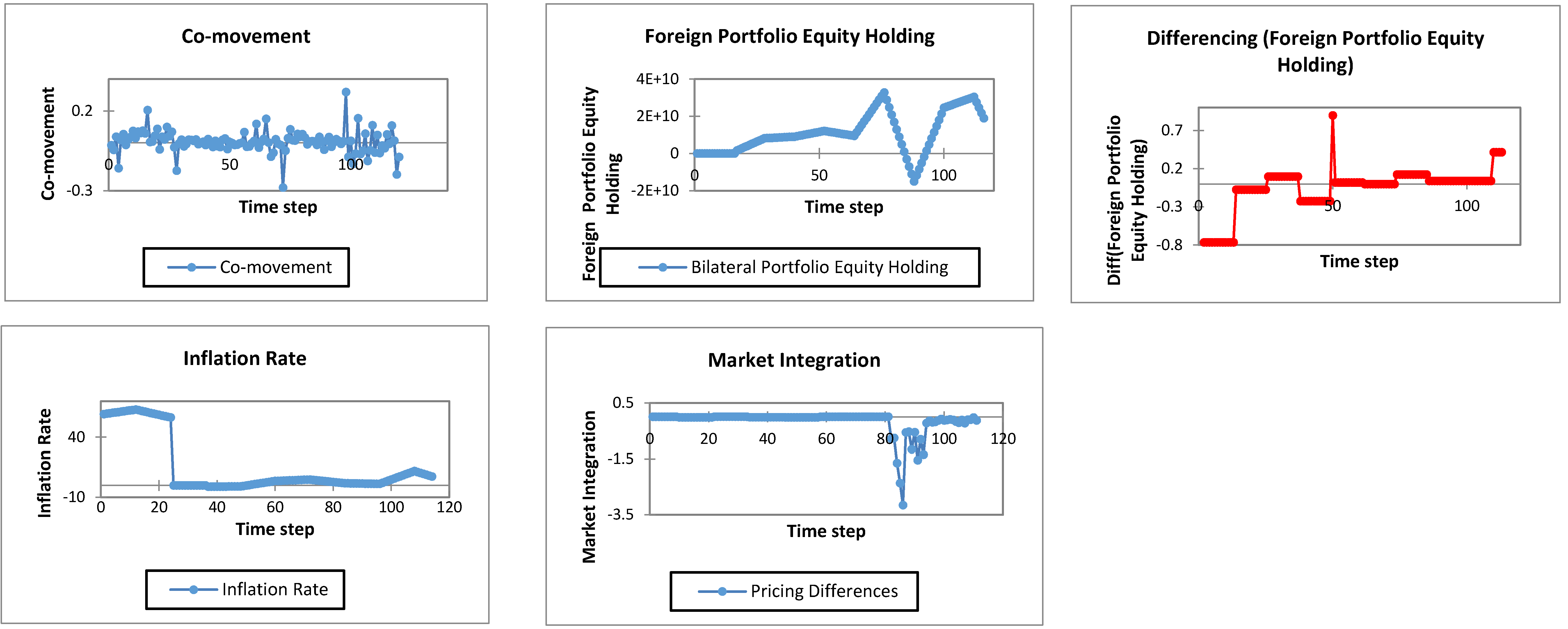
In this paper, we have applied ARDL technique. From

Table 2. ADF statistics and Mackinnon (1996) one-sided p-values.

Variables	At-Level	At First Difference
Return Co-movement	−9.4557 *
Foreign Portfolio Equity Holding	−1.2174	−4.4369 *
Market Integration	−4.5892 *
Inflation Rate	−3.3950 *

Notes: * represents the rejection of null hypothesis at one percent level.

, it is evident that our variables exhibited stationarity at different levels. Foreign portfolio equity holding was stationary at first difference, whereas all the other variables are stationary at level. ARDL techniques deal with this issue of stationarity at different levels. This is the reason we applied ARDL technique. If all of our variables were stationary at the same level, we would have applied Johansen cointegration technique. Further illustration of the stationarity properties of included variables is presented in Figure 1.

As all the variables are stationary at level and first difference, we have applied auto regressive distributed lag (ARDL) model to check the short and long run relationship among them. The application of ARDL approach has many benefits and ease of operation as compared to the traditional co-integration approaches. The traditional co-integration tables require the same level of integration among the associated variables whereas we can apply auto regressive distributed lag (ARDL) model at different levels of stationarity2. Another benefit of the application of ARDL model is its application on short time series as compared to the co-integration techniques that require long time series data sets [38]. The ARDL approach helps in capturing the long run relationship among the associated variables integrated at different levels. Further, the application of unrestricted error correction model (UECM) can capture the dynamics of both short and long term relationship.

We have applied ARDL3 bound testing for analyzing the relationship between Indian and Pakistani stock markets.

Table 3. Lag order selection criteria.

Lag	LR	FPE	AIC	SC	HQ
0	NA	0.001	3.871	3.968	3.910
1	1042.06	0.000	−5.582	−5.097	−5.385
2	355.355	0.001 *	−0.008 *	−0.007 *	−0.008 *
3	16.860	0.000	−8.631	−7.369	−8.119
4	11.863	0.000	−8.470	−6.820	−7.801
5	39.653	0.000	−8.620	−6.581	−7.793
6	14.742	0.000	−8.504	−6.077	−7.519
7	27.540 *	0.000	−8.550	−5.735	−7.408
8	12.003	0.000	−8.416	−5.212	−7.116

LR represents Sequential Modified Test Statistics; FPE represents the Final Prediction Error; AIC represents Akaike Information Criteria; SC represents Schwarz Information Criteria; HQ represents Hannan Quinn Information Criteria; * represents the lag order selected.

shows the lag selection criterion that has been applied to ARDL approach and lags up to second term is included based on Sequential modified test statistics, Schwarz information criteria and Hannan information criteria. The resultant equation4 that is estimated after the above-mentioned lag selection is presented below.

$$\Delta SM{C}_t={\alpha }_0+{\alpha }_{1}SM{C}_{t-1}+{\alpha }_{2}M{I}_{t-1}+{\alpha }_{3}FPE{H}_{t-1}+{\alpha }_{4}I{R}_{t-1}+{\displaystyle \sum _{i=1}^p}{\theta }_1\Delta SM{C}_{t-i} {\displaystyle \sum _{i=0}^q}{\theta }_2\Delta M{I}_{t-i}+{\displaystyle \sum _{i=0}^u}{\theta }_3\Delta FPE{H}_{t-i}+{\displaystyle \sum _{i=0}^w}{\theta }_4\Delta I{R}_{t-i}+trend+{\mu }_t$$

(4)

The null hypothesis presented above states that there is no long term relation among the associated variables in lights of the values presented by Pesaran et al. [34]. For long term relationship between these variables, the critical value mentioned in

Table 4. ARDL bound test critical values.

Critical Values	90 Percent		95 Percent		99 Percent
	Lower Bounds	Upper Bounds	Lower Bounds	Upper Bounds	Lower Bounds	Upper Bounds
	I(0)	I(1)	I(0)	I(1)	I(0)	I(1)
Return Co-movement	2.68	3.53	3.05	3.97	3.81	4.92

has lower bound value of 3.05 and an upper bound value of 3.97 at five percent significance level. The value that we have obtained from Wald test statistics gives us a value of 21.021 significant at five percent level greater than the critical value at upper bound indicating long term relation among the variables. Results of

Table 5. ARDL Model.

Regressor (1,1,2,1) Based on SBC	Coefficient	Standard Error	T Ratio
Constant	0.013	0.013	1.042
D(SMC(−1))	0.179	0.095	1.883
D(MI)	0.0232 *	0.0159	1.4591
D(MI(−1))	0.0538 *	0.0047	11.447
D(FPEH)	0.0012	0.0198	0.0606
D(FPEH(−1))	1.295 *	1.664	0.778
D(FPEH(−2))	−3.950 *	1.686	−2.344
D(IR)	−0.068 *	0.047	−1.455
D(IR(−1))	0.004 *	0.062	0.061
TREND	−0.0002 *	0.0002	−1.0612
R-squared	0.6206
Adjusted R-squared	0.5908
Akaike info criterion	−2.1593
Schwarz criterion	−2.9829
F-statistic	12.546
F-significance	0.0000
Durbin-Watson stat	1.9439
Breusch-Godfrey LM test	0.2991
Wald Test	21.0208 *

Notes: * represents the rejection of null hypothesis at one percent level.

shows that coefficient value of all the included variables is statistically significant.

The above table presents the critical values given by Pesaran et al. [34] in the presence of restricted trend and unrestricted intercept term in the equation. The hypothesis that is be tested for the ARDL bound testing in this and the subsequent section is presented below.

$$\begin{array}{ccc}{H}_0:{\alpha }_1={\alpha }_2={\alpha }_3={\alpha }_4=0& & (\text{No cointegration})\end{array}$$

(5)

Results of long term coefficients in

Table 6. Estimated long run coefficients for selected ARDL model.

Regressor	Coefficient	Standard Error	T Ratio
MI	0.0129	0.120	0.108
FPEH	1.7326 *	0.961	1.803
IR	1.2306 *	0.010	123.1

Notes: * represents the rejection of null hypothesis at one percent level.

under the ARDL approach shows that in long run inflation rate differential and Foreign portfolio equity holding between India and Pakistani equity markets has significant positive relationship with the bilateral stock market co-movement. Market integration between the two countries are positively related but with insignificant values. We have also checked our model for serial correlation through Breusch-Godfrey LM test and it can be seen that its value is insignificant at one percent significance level, accepting the null hypothesis of no serial correlation.

Table 6 shows us the long run of bilateral stock market co-movement with all of the included independent variables (i.e., market integration, financial integration and inflation rates). In Table 6, there is a long run relationship between co-movement and inflation rate differential. This relationship indicates that if the inflation rate differences between the associated countries increases, bilateral stock market co-movement will also increases. This might be attributed to the shifting of investors due to differing interest rates thereby resulting in stock market synchronicity.

Table 7. Error correction representation for the selected ARDL model.

Regressor	Coefficient	Standard Error	T Ratio
Constant	0.0189	0.0098	1.9397
D(SMC(−1))	0.1703	0.0940	1.8114
D(MI)	0.0022 *	0.0061	0.3700
D(MI(−1))	−0.0009 *	0.0060	−0.1481
D(FPEH)	0.0068 *	0.0036	1.8917
D(FPEH(−1))	0.3204*	0.1892	1.6935
D(FPEH(−2))	1.295	1.664	0.778
D(IR)	−3.950 *	1.686	−2.344
D(IR(−1))	−0.068 *	0.047	−1.455
TREND	0.004 *	0.062	0.061
ECT(−1)	−0.7659 *	0.1348	−9.2074
R-squared	0.5883
Adjusted R-squared	0.5451
Akaike info criterion	−3.2507
Schwarz criterion	−2.9674
F-statistic	13.6384
F-significance	0.0000
Durbin-Watson stat	1.9179
Breusch-Godfrey LM test	1.9800
Wald Test	4.4636 *

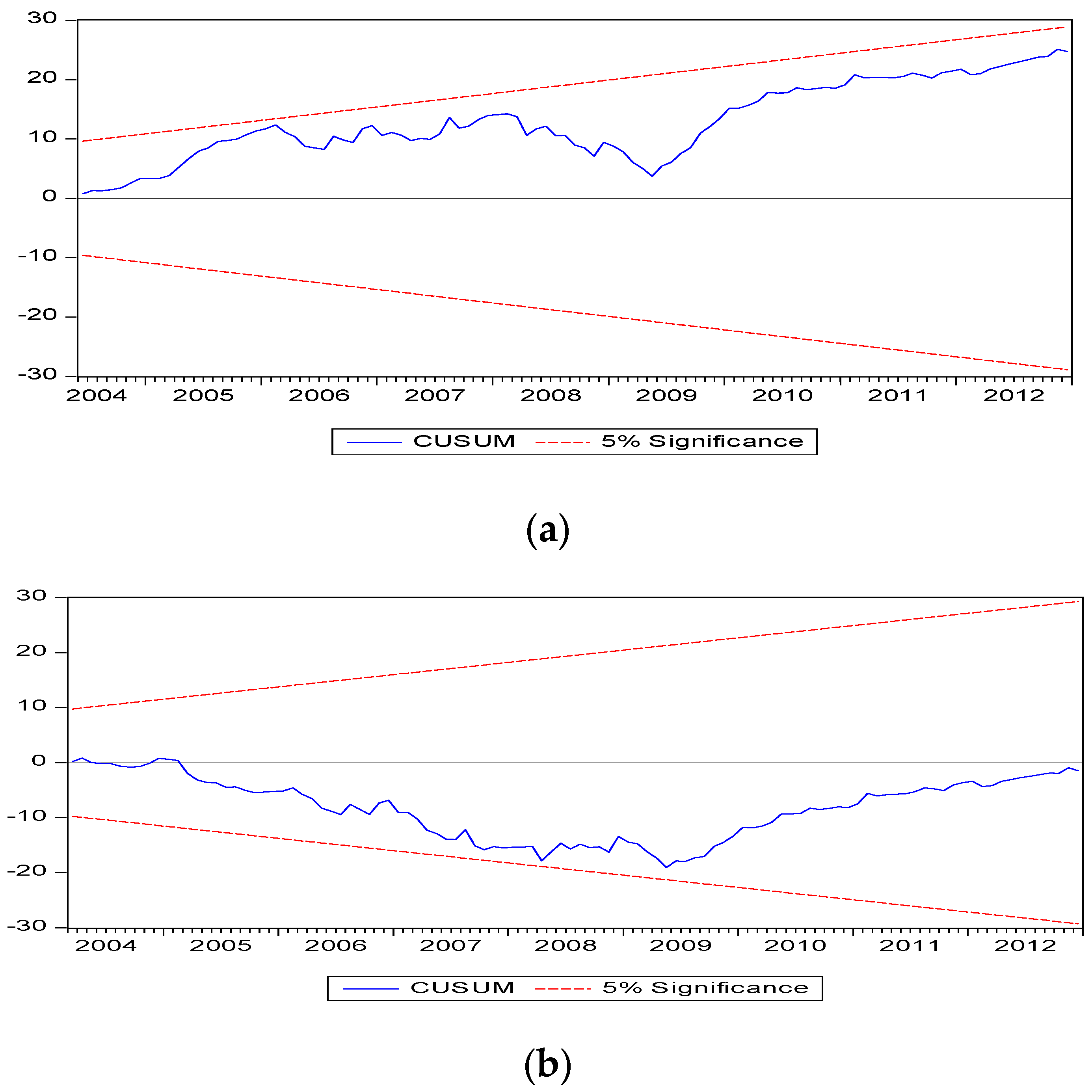
Notes: * represents the rejection of null hypothesis at one percent level.

also reports significant short run relationship between bilateral co-movement and inflation rate differential but only for a single lag value. It can be seen in Figure 2a that our model is quite stable as the line is sandwiched between the two boundaries in both upper and lower levels. Furthermore, we have introduced Error Correction Term (ECT) in our model to check the short term relationship between our variables. The expression for the error correction term in our model is presented below.

$$\Delta SM{C}_t={\alpha }_0+{\sum }_{i=1}^p{\theta }_1\Delta SM{C}_{t-i}+{\sum }_{i=0}^q{\theta }_2\Delta M{I}_{t-i}+{\sum }_{i=0}^u{\theta }_3\Delta FPE{H}_{t-i}+{\sum }_{i=0}^w{\theta }_4\Delta I{R}_{t-i}+trend+{\beta }_{1}EC{T}_{t-i}+{\mu }_t$$

(6)

where,

$$EC{T}_{t-i}={\alpha }_{1}SM{C}_{t-1}+{\alpha }_{2}M{I}_{t-1}+{\alpha }_{3}FPE{H}_{t-1}+{\alpha }_{4}I{R}_{t-1}$$

Error correction coefficients of the above mentioned short term representation is reported in Table 7. Foreign portfolio equity holding is the only variable that has significant positive relationship with bilateral stock market co-movement.

The value of coefficient in the error correction term is −0.6791 with high significance level and the speed of adjustment is 77 percent. The short term relationship among the included variables, represented by Wald test, is 1.9800. Breusch-Godfrey test suggests that our model including error correction term has no serial correlation and Figure 2b also shows that our model is quite stable.

3.3. Variance Decomposition Analysis

Table 8. Variance decomposition analysis.

Period	S.E.	SMC	MI	FPEH	IR
1	0.047	93.393	0.349	0.000	0.047
2	0.049	90.783	1.992	4.957	0.049
3	0.050	87.066	5.366	7.618	0.050
4	0.051	84.197	7.484	9.173	0.051
5	0.051	82.570	8.716	10.477	0.051
6	0.052	81.478	9.442	11.376	0.052
7	0.052	80.745	9.784	11.938	0.052
8	0.052	80.262	9.872	12.273	0.052
9	0.052	79.896	9.844	12.451	0.052
10	0.052	79.542	9.810	12.527	0.052

S.E. represents Standard error; SMC represents Stock Market Co-movement; MI represents Market Integration; FPEH represents Foreign Portfolio Equity Holding; IR represents Inflation Rate Differential value.

presents the result of variance decomposition test in explaining the bilateral stock market co-movement. In the short run, self-variance of return co-movement is almost 100 percent, which reduces to almost 80 percent in the long term. Aside from self-variation by bilateral stock market co-movement, none of the variables has induced notable variation in bilateral co-movement in short term.

In the long run, maximum variation of 9.81 percent is provided by market integration. Foreign portfolio equity holding has 13 percent variation, whereas market integration has a nominal variation of one percent in the bilateral stock market co-movement. All of the above statistics suggest that as far as the Pakistani investors are concerned with making equity investments in India stock markets, Foreign portfolio equity holding provide maximum variation in the bilateral co-movement in long run; however, no significant variation is provided either by market integration and inflation rate differential. Therefore, as far as diversification benefits are concerned, the model captures variation only from foreign portfolio equity holding in bilateral stock market co-movement unlike rest of the variables.

4. Conclusions and Discussion

The purpose of this study is to explore the factors playing important roles in bilateral stock market co-movement between Indian and Pakistani stock markets. In the case of developed markets under the efficient market hypothesis, stock markets are considered as an economic indicator, whereas in the case of developing and emerging markets, other factors can be influential. This study aims to capture the role of market integration, foreign portfolio equity holding and inflation rate differences on bilateral stock market co-movement. Findings of this study suggest that both long and short term relationship exists among these variables with positive effect of both market integration and foreign portfolio equity holding. This study highlights that with an increasing gap of inflation rates between these two countries, co-movement tends to increase so investors should monitor the changes in inflation rates before making any long and short term investments. Similarly, market integration and foreign portfolio equity holding tends to increase the bilateral equity co-movement. As both of these markets are categorized as emerging markets (Morgan Stanley Classification Index), these factors are very important to predict the bilateral return co-movement among the stock markets of Pakistan and India. Future research in the same area can also include more countries in the analysis in the form of panel which can be generalized to the overall Asian region including all the emerging and frontier markets. Furthermore, the co-movement pattern of Asian emerging and/or frontier markets with the developed markets, i.e., European and the US markets can be determined. Finally, many of the other financial, market or macroeconomic variables can be included in the analysis.