Abstract
Undiversifiable (or systematic risk) has long been an enemy of investors. Many countercyclical strategies have been developed to counter this. However, like all insurance types, these strategies are generally costly to implement, and over time can significantly reduce portfolio returns in long and extended bull markets. In this paper, we discuss an alternative technique, founded on the premise of physiological bias and risk-aversion. We take a behavioral discussion in order to contextualize the insurance like characteristics of option pricing and discuss how this can lead to a mispricing of the asymmetric relationship between the VIX and the S&P 500. To test this, we perform studies in which we find statistical inefficiencies, thereby making it possible to implement a method of hedging index option premium in a way that has displayed no monthly drawdowns in bullish periods, while still providing large returns in major sell-offs. The three versions of the strategy discussed have negative betas to the S&P 500, while exhibiting similar risk-adjusted excess returns over both bull and bear markets. Further, the performance generated over the entire period, for all three strategies, is highly statistically significant. The results challenge the weak form of the Efficient Market Hypothesis and provide evidence that the methods of hedging could be a valuable addition to an equity rich portfolio for the purpose of counteracting systematic risk.
JEL Classification:
G01; G02; G11; G14
1. Preface
At the time of writing (Q1, 2015), interest rates are near record lows and “all major economies have higher levels of borrowing, relative to GDP, than they did in 2007” [1]. The authors argue that an alternative investment approach, such as the one presented in the paper, may be particularly attractive if the market turns out to have too much debt; which may force market participants into protective (but costly) hedging. This paper explores a proactive approach to this problem that has shown evidence of working well in the past. The results, applicability and considerations are set in light of a behavioral finance approach, leading to discussions that are intended to help market practitioners make more informed decisions in the context of counteracting systematic risk.
Note: The original study was performed in late 2014, a follow up “out of sample” study has now been performed, showing continued performance against systematic risk. This section is included after the conclusion.
2. Introduction
Recent developments in the behavioral sciences have shown that losses create a negative physiological impact of approximately double the magnitude of the positive impact we would experience from an equal gain. This finding showed that we are inherently loss averse and is in essence the basis of Tversky and Kahnemans Prospect Theory. As the options market is fairly new, and still developing in terms of various pricing models, we thought it would be interesting to test whether the predictable loss aversion preference is evident and accurately priced into the market. In this article, we set out to achieve this through the empirical study of three strategies, all of which take positions in put options on the S&P 500 ETF (ticker: SPY) hedged against call options in the VIX, or VXX (which is a ETN that closely follows the movement of the VIX, as it holds positions in front and back month VIX futures).
The VIX (commonly referred to as the fear index) and the S&P 500 are known to have a strong inverse relationship. However, what makes this relationship interesting is that the VIX derives its price from the options on the S&P 500, which is something that gives these two products a fundamental link. The VIX is calculated by the CBOE in such a way to give a forecast of the coming 30-day volatility in the S&P 500. As options are well known for their “insurance like” characteristics, the level of the VIX can be seen as a measure of the cost to insure the S&P 500 at a given point in time. There are two main aspects of this relationship that make for an interesting study. First, given its common name of “the fear index”, is this relationship susceptible to loss aversion? Second, if loss aversion does influence the interpretation of the relationship, do prior gains or losses frame the choice set and lead to a miss-pricing of risk? To put this in context, one of the corner stone principles of Neoclassical Economics and the assumptions made in the Efficient Market Hypothesis are that market participants are rational. If this were indeed the case, the pricing of the relationship would not be predictably affected by loss aversion in such a way that one could beat the benchmark by trying to take advantage of it, as the risk would be accurately priced into the market. This would support a null hypothesis that no significant risk-adjusted excess returns could be generated by specifically trying to exploit this relationship.
As an alternative to this, we put forth that: (1) loss aversion is likely to drive the VIX to spike more than it “rationally” should during a market crash, as it causes market participants to evaluate the probability and weight of future outcomes incorrectly, which increase the demand for insurance (put options); and, (2) prior to such an event occurring, positive market developments may frame the choices and lead to market participants underestimating the likelihood and psychological impact of an extreme event. Such a case would likely lead to an underpricing of VIX and VXX out-of-the-money call options relative to out-of-the-money SPY put options.
This study examines whether this alternative hypothesis can be substantiated, and if so, understand whether such strategies can be used to combat systematic risk on a month-to-month basis.
3. Literature Review
As examined by a multitude of scholars [2,3,4,5,6,7], the demand for increased protection during market declines results in an asymmetric relationship between implied volatility and the underlying price—a phenomenon known as volatility asymmetry. We find that despite this relationship being well documented, option prices on the S&P 500 and the VIX have inadequately reflected these dynamics, even after similar observations were previously noted [7] 1. This has given rise to the strategies discussed in this paper, all of which have functioned as an effective counter to systematic risk.
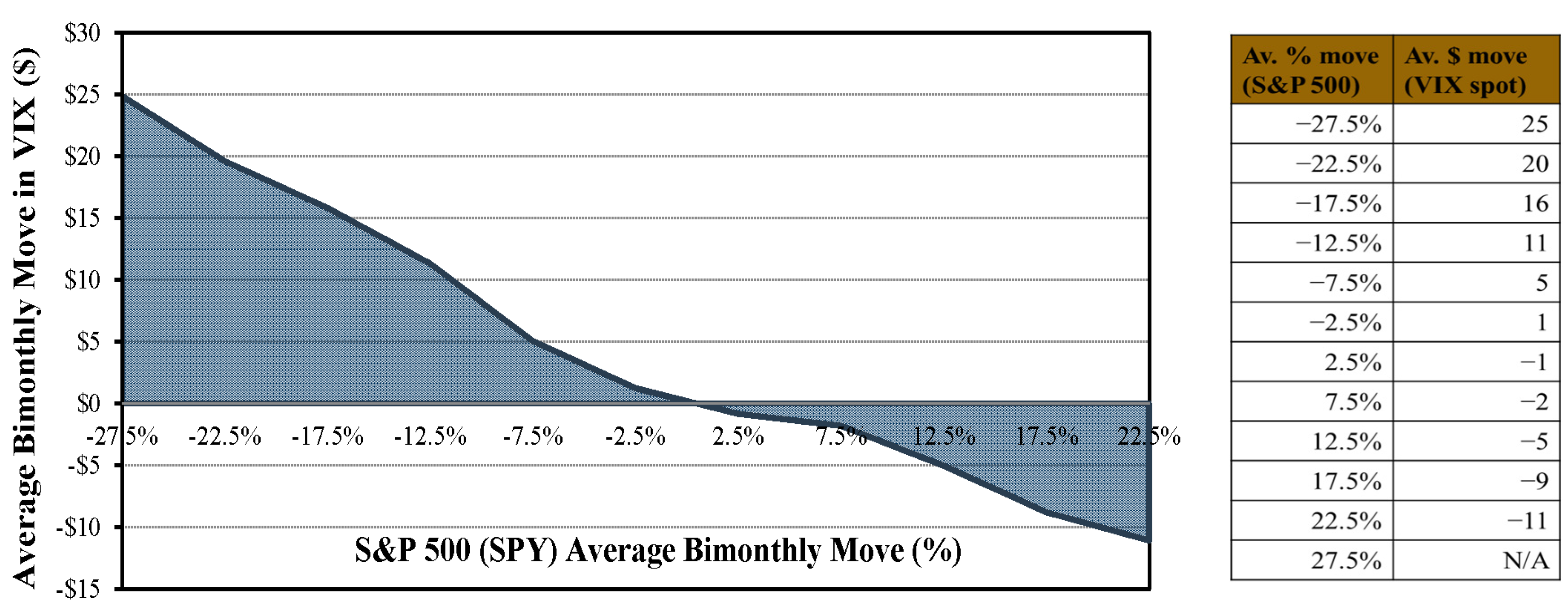
As can be seen below in Figure 1, the VIX has a tendency to rise and fall with a disproportionate magnitude to that of the market, even before the 2008 crisis.

Figure 1.
Bimonthly Asymmetric Relationship—Spot VIX to S&P 500 (1993–2006). This chart shows the asymmetric relationship of the VIX and S&P 500 (1993–2006) prior to the study period of the strategies dealt with in this paper (2006–2014). The reason for visualizing this particular time period is to show that this asymmetric relationship was present before VIX futures, or VIX options, were available for trading—thereby implying that it should be priced into the subsequent VIX derivatives to the extent where consistent significant risk-adjusted excess returns are impossible to achieve by specifically trying to take advantage of it. The pricing of this subsequent relationship is central to this paper. Sources: CRSP and CBOE.
Furthermore, it is common knowledge that option prices are largely dependent on perceived probabilities and demand for certainty, and thus can be used as a form of insurance. We argue that is in line with the work of Jackwerth [6] who, in his paper on recovering risk aversion, notes that a relationship exists between the aggregate risk-neutral probability, the subjective probability distributions and the risk aversion functions across wealth. Based on these factors an equation was formulated, which we have tailored into the notation below:
where P is risk-neutral probability; is subjective probability; and R is risk aversion adjustment.
Jackwerth [6] explained that the risk neutral probability (P) is the price that the investor would pay to receive one dollar, taking into account the risk free rate of return at a specified point in time. The subjective probability ( is the investor’s biased evaluation of likelihood of occurrence, and the risk aversion adjustment (R) relates directly to the individual risk profile of the investor. Further, he noted the differences in the risk-neutral distributions before and after the crash in 1987. Finding that implied risk aversion functions were dramatically altered to an extent where investors were exhibiting greater risk aversion after this crash. In Figure 1, we see a similar dynamic risk averse pattern emerge in the form of the demand for protection in market declines. This is reflected by an almost twofold increase in implied volatility (VIX) in market declines vs. the decrease in market inclines. What we put forth is that P has a large effect on option pricing due to, (1) the reliance on variables that are highly dependent on the subjective interpretation of the relative frequency of past events; (2) their projection as a predictor of future probabilities; and (3) the degree of loss aversion that the investor is displaying. If we examine the variables that comprise this risk-neutral probability , it becomes apparent that their interplay (when determining the risk-neutral probability in changing market environments) can bring about interpretational biases specifically with regards to the pricing of risks. Further, it was noted that initial losses tend to increase the temerity with which we can say that people become increasingly risk-averse [8], which reflects the relationship we see between volatility and the market. We argue that this could become even more apparent in economies of high leverage, due to a forced demand of protective hedging in order to meet debt obligations, which is especially likely if sell-offs threaten the livelihoods of investors. This is in line with Shiller’s thoughts from his book Irrational Exuberance, in which he states, “More and more electronic markets are being created every year, trading a wider and wider range of risks, and more and more people, in both advanced and emerging countries, are being drawn in to participate in these markets. People will increasingly fear that their livelihoods really depend on their wealth, wealth that is highly unstable because of market changes. People increasingly believe that they must defend their private property and doubt that they can depend on social institutions if things turn out badly” [9].
The Shiller P/E (CAPE) ratio, at the time of writing, is at 2007 levels (27,67) [10] and high global economic leverage has been documented by the McKinsey Global Institute [1]. Given these measures, it is perhaps a reasonable concern that any correction of valuations may result in an amplified risk-aversion adjustment. Therefore, we consider it an appropriate time to discuss alternative techniques that are likely to benefit from such conditions.
The strategies subsequently evaluated and discussed, have delivered small but consistent total returns during bullish conditions, and significantly greater returns in large market wide sell-offs. The core hedge principles of the strategies are built around the asymmetrical relationship between the S&P 500 and the VIX. We show that these strategies have been consistently profitable through a range of market conditions, arguably due to the failure of the market participants to accurately price in this asymmetric relationship. The strategies function as a means to achieve statistical arbitrage from the market’s relationship with its implied volatility, and therefore termed Volatility Beta-Arbitrage. All positions are constructed exclusively from contract options on the underlying assets: SPY, VIX and VXX. All three of the evaluated versions of the strategy exhibit risk-adjusted excess returns that are robust over varying market conditions and are highly statistically significant.
4. Strategy Methodology
Three separate strategies with different properties were tested, we refer to each of them by the notations below:
VBA (NH): Volatility Beta-Arbitrage—Normal Hedge strategy (using VIX options for hedging index premium).
VBA (TH): Volatility Beta-Arbitrage—Tail Hedge strategy (using VIX options, but with adjustments to VBA (NH) strike parameters).
VBA (NHTL): Volatility Beta-Arbitrage—Normal Hedge, Triple Leverage strategy (using VXX options. The strike selection is based on the same parameters as VBA (NH), but performance is calculated with one third of the margin allocation).
As a means of reducing errors, option data were compared between two different sources (Option Metrics and the CBOE). CRSP was used as the source for the underlying assets SPY and VXX, while the CBOE was used to obtain VIX futures prices 2. In order to obtain our results, positions on the SPY and VIX or VXX options, with two months until expiration, were calculated for each variation of the strategy on a monthly basis. Trades were opened on the first Monday (or closest business day) after the monthly option expiration cycle (the third Friday of each month) and held until their expiry. An exception to this was when utilizing VIX options, as these options expire on the Wednesday before (or after) SPY option expiration. In these cases, to prevent any strategy from being unhedged, positions were taken off at the first option expiration date.
In order to measure the compounded performance against the benchmark, the monthly staggered performance of each strategy was tested as a combined portfolio. Meaning that trades were initiated once a month and then held until expiry (approximately 60 calendar days per trade); we refer to this as “staggering”. The profit or loss from the previous month was then reinvested into each subsequent month in order to give a realistic compounded performance progression of each portfolio. The combination of the two parallel trade cycles were then combined, forming one portfolio per strategy (the entire compounded development of each strategy, measured in this manner, is represented in the chart in Appendix D).
An example below (Figure 2) to illustrate trade staggering in a portfolio over a four-month period:

Figure 2.
Trade staggering in a portfolio over a four-month period.
Figure 2.
Trade staggering in a portfolio over a four-month period.

During the data screening, mid-prices were calculated in order to reduce the “bid-ask bounce bias”. Further, transaction costs and possible slippage was accounted for by deducting 20 USD per single monthly position and this was incorporated into the performance evaluation of all of the strategies. The monthly positions were calculated as a trade ratio of the nearest-to-the-money put option for a given position. The following template formula was used to determine the correct ratio of SPY puts to volatility calls to be bought or sold each month:
where:
and:
- = One nearest-to-the-money SPY put option, Z percentage out-of-the-money (constant);
- = The ratio of volatility call option(s), Z percentage out-of-the-money;
- = The ratio of the furthest-from-the-money SPY put option(s), Z percentage out-of-the-money;
- = The price of one nearest-to-the-money SPY put option, Z percentage out-of-the-money;
- = The price of one volatility call option, Z percentage out-of-the-money;
- = The price of one furthest-from-the-money SPY put option, Z percentage out-of-the-money;
- x = A set parameter defining the ratio between the price of a volatility call option and a nearest-to-the-money put option. Referred to as volatility coverage ratio 3.
- y = A set parameter defining the ratio between the price of the furthest out-of-the-money SPY put option to the combined cost of the bought options in the position, therefore referred to as the credit ratio 4.
- Matrix for Z, to denote percentage out-of-the-money.
4.1. Volatility Beta-Arbitrage Strategy Specifics
4.1.1. Strategies Using VIX Options, VBA (NH) and VBA (TH)
In order to calculate the bimonthly return on capital for each position, despite the ratio changes (different prices result in a changing number of option contracts to buy and sell each month), a margin allocation of $35,000 per “single monthly position” was used throughout the test period. The rationale behind choosing this allocation amount was to construct a safe position (concerning the amount of leverage used) that could easily account for ratio fluctuations in a live scenario even with stringent margin requirements. This also has the advantage that if volatility were to rise less than anticipated, the generous capital allocation would keep the risk of the trade to a minimum 5.
Formula specifics for VBA (NH): the ratios for VBA (NH) were based specifically on trades that had shown robust live performance in the market. The strategy specific variables, constant for the entire test period, were as follows: for volatility calls VIX options were used, x and y were both set to 110%. Regarding the appropriate out-of-the-money strike percentage selection, the following parameters for each of the variables were chosen: , and . At the start of each month (from October 2006–October 2014), the nearest possible strike for each of the strike variables were selected and the performance tracked.
Formula specifics for VBA (TH): the adjusted strategy specific variables, constant for the entire test period, were as follows: for volatility calls VIX options was used, x was set to 100% and y set to 150%. Regarding the appropriate strike selection, the following parameters for each of the variables were chosen: , and . At the start of each month (from October 2006–October 2014) the same approach as above was applied.
4.1.2. Strategy Using VXX Options, VBA (NHTL)
For the third strategy VBA (NHTL), approximately one third of the capital was allocated to each position ($11,700). This had the effect of tripling the leverage in the position, making it more volatile, but also increasing potential returns—making for an interesting evaluation study.
Formula specifics for VBA (NHTL): the strategy specific variables were the same as for VBA (NH) except instead of VIX options, VXX options were used, and performance was tracked accordingly (October 2010–October 2014).
5. Performance of the Strategies (Results)
If any meaningful weight is to be attached to a claim of market out-performance of a strategy, it is important to compare the performance relative to that of a relevant benchmark. In this case the S&P 500 ETF (SPY) is the natural choice of benchmark, as the risk of each strategy is derived solely from its price at option expiry. In order to calculate the risk-adjusted excess returns, the bimonthly excess returns of each strategy can be analyzed for their relationship with the benchmark by means of a time-series regression (Equation (3)). If the benchmark fully explains the risk of the strategy, the average risk-adjusted excess return of each strategy should be equal to zero; this is in line with Neoclassical assumptions and EMH. If it is positive, it implies that the strategy is earning returns over and above the risk taken, which should not be consistently possible in a martingale. This would imply our alternative and the susceptibility to behavioral basis as described in the Introduction. If there were doubt as to whether the benchmark (SPY) was fully inclusive of the risk in the strategies, a multi-factor model would be considered as a supplement to the results. However, in this case, the single-factor model fits our purposes because the risk factor is the benchmark return. Given that the realized excess returns of the strategies, at expiration, are being regressed by the model—as compared to the raw excess returns of the benchmark—we consider the model to be appropriate for the purposes of identifying the alpha, beta and significance. With this in mind, the following null and alternative hypotheses are set up in order to test each strategy for its risk-adjusted excess return:
- H0: The mean risk-adjusted excess return of the strategy is zero.
- H1: The mean risk-adjusted excess return of the strategy is not zero.
The null hypothesis is tested for all three strategies by means of the below time series regression (Equation (3)), which examines the relationship between the realized bimonthly excess returns of each strategy and the corresponding excess returns of the benchmark, over the same period.
where:
- R = Bimonthly excess return of the strategy;
- Risk-adjusted excess return of the strategy (x-intercept of the regression);
- Beta coefficient of the strategy’s excess return measured against the benchmark’s excess return (slope of the SML);
- Bimonthly excess return of the market (benchmark);
- e = Standard error of the bimonthly risk-adjusted excess return of the strategy.
5.1. The Performance of the Volatility Beta-Arbitrage (Normal Hedge) Strategy
Table 1 summarizes the key results of the regression for VBA (NH), as well as the risk and return statistics over the entire test period. As can be seen, the average bimonthly risk-adjusted excess return (α) over the 95-month period is 1.5%, with a p-value of 0.00098—which gives the performance statistical significance—permitting us to reject the null hypothesis at a confidence level in excess of 99.90%. A comparison was made between the performance of the strategy under both bearish and a bullish market conditions. For these purposes we considered the period October 2006–October 2010 as being predominantly bearish, in which we found a bimonthly risk-adjusted excess return of 1.38%, while in the subsequent bullish period October 2010–October 2014 we found a very similar bimonthly performance of 1.30%. Based on this, we concluded that the strategy yielded positive risk-adjusted excess returns over varying market conditions.

Table 1.
Bimonthly Performance of Volatility Beta-Arbitrage—Normal Hedge (October 2006–October 2014).
| Key Regression Results | ||
| α (%) | 1.500 | |
| p-value of α (#) | 0.001 | |
| Std. Error (#) | 0.004 | |
| β (#) | −0.340 | |
| Risk and Return | ||
| Measure | M * | VBA (NH) ** |
| Annual compound growth rate (%) | 6.20 | 7.50 |
| Standard deviation, daily returns (%) | 22.10 | 8.10 |
| Sharpe *** (#) | 0.24 | 0.82 |
| Total months traded (#) | 95 | 95 |
| Total return, months positive (#) | 63 | 93 |
| Total return, months negative (#) | 32 | 2 |
* Benchmark (S&P 500); ** Volatility Beta-Arbitrage Strategy (Normal Hedge); *** Average risk free rate over entire test period used for calculation. # denotes numerical form.
Considering the risk and return measures over the eight-year period, the strategy exhibited negative total returns in only two of the 95 months, in contrast to the 32 negative months experienced by the benchmark. This is especially attractive when considering the negative β with the market, and zero negative months during the bullish period. Comparing the return and variance results 6, we see the strategy exhibited lower risk and higher return statistics than the benchmark, resulting in its Sharpe ratio being over three times higher than that of the S&P 500—again pointing to the attractiveness of the strategy.
5.2. The Performance of the Volatility Beta-Arbitrage (Tail Hedge) Strategy
Table 2 summarizes the key results for VBA (TH). With the average bimonthly risk-adjusted excess return over 2% we find a considerable market outperformance over the entire period (October 2006–October 2014), and with a p-value of 0.00169, this is highly statistically significant—again permitting us to reject the null hypothesis with over 99.83% confidence. Performance, when adjusting for market risk, was also positive in both bull and bear markets. Although average bimonthly risk-adjusted excess returns of 1.9% during the bear market was considerably more than average bimonthly performance of 0.5% during the bull market. This “market insurance” characteristic of the strategy is also apparent from the β of close to −0.6.

Table 2.
Bimonthly Performance of Volatility Beta-Arbitrage—Tail Hedge (October 2006–October 2014).
| Key Regression Results | ||
| α (%) | 2.033 | |
| p-value of α (#) | 0.002 | |
| Std. Error (#) | 0.006 | |
| β (#) | −0.596 | |
| Risk and Return | ||
| Measure | M * | VBA (TH) ** |
| Annual compound growth rate (%) | 6.20 | 7.90 |
| Standard deviation, daily returns (%) | 22.10 | 7.20 |
| Sharpe *** (#) | 0.24 | 0.98 |
| Total months traded (#) | 95 | 95 |
| Total return, months positive (#) | 63 | 93 |
| Total return, months negative (#) | 32 | 2 |
* Benchmark (S&P 500); ** Volatility Beta-Arbitrage Strategy (Tail Hedge); *** Average risk free rate over entire test period used for calculation. # denotes numerical form.
What makes this an especially attractive counter to systematic risk, is that despite the substantially negative β, there were no negative months during the bullish period, and returns were of low volatility; note the Sharpe ratio 0.98.
5.3. The Performance of the Volatility Beta-Arbitrage (Normal Hedge, Triple Leverage) Strategy
The results displayed in Table 3 show the performance of the third strategy VBA (NHTL). Due to the increased leverage of the strategy, we see a highly attractive bimonthly performance of close to 5%. This is attained with a p-value of 0.00017, meaning that it has an even higher statistical significance than the previous two strategies, allowing a rejection of the null hypotheses at a confidence level over 99.98%. Due to the leverage, β decreased even further to negative 0.84, which becomes a highly attractive prospective portfolio addition, considering that this was achieved with no realized monthly losses over a 47-month bullish period. The Sharpe ratio is not quite as attractive as that of the market, but when considering that due to the zero negative total returns, most of the volatility occurred to the “up-side”, the strategy makes a strong case to its application and relevance for diversifying a market portfolio.

Table 3.
Bimonthly Performance of Volatility Beta-Arbitrage—Normal Hedge, Trip L. (October 2010–October 2014).
| Key Regression Results | ||
| α (%) | 4.973 | |
| p-value of α (#) | 0.000 | |
| Std. Error (#) | 0.012 | |
| β (#) | −0.840 | |
| Risk and Return | ||
| Measure | M * | VBA ** (NHTL) |
| Annual compound growth rate (%) | 14.70 | 15.90 |
| Standard deviation, daily returns (%) | 15.30 | 19.20 |
| Sharpe *** (#) | 0.95 | 0.82 |
| Total months traded (#) | 47 | 47 |
| Total return, months positive (#) | 37 | 47 |
| Total return, months negative (#) | 10 | 0 |
* Benchmark (S&P 500); ** Volatility Beta-Arbitrage Strategy (Normal Hedge Trip. L.); *** Average risk free rate over test period used for calculation. # denotes numerical form.
5.4. Summary of Performance
The two strategies that were possible to trade during both bull and bear markets, exhibited positive risk-adjusted excess returns over different market conditions and time-periods (this is in contrast to the weak form of EMH, which states that past performance should already be incorporated into prices). Moreover, by adjusting the core hedge (as in VBA (TH)) and using the initial strategy hedged with options on different volatility products (VBA (NHTL)), the chance of the results being down to a statistical anomaly or luck, is vastly reduced. The level of significance that the performance has shown, clearly points to their attractiveness as a quotidian diversification tool in a market exposed portfolio. Nonetheless, it is important to understand the mechanics behind this type of alternative diversification method and the assumptions that need to be made for such performance to continue, so that informed trading decisions can be made.
Considerations: While our study did incorporate the lead up to the 2008 crisis with more “normal” interest rates, a long stretch of higher rates may reduce excess returns. Further, it should also be kept in mind that given that VIX options were only available from 2006 and VXX options from 2010, we are not able to do further studies in generally higher interest rate environments to establish or falsify this.
For readers interested, further statistics are incorporated in the Appendices A–C showing the regression output as well as a visualization of bimonthly returns for all strategies against the benchmark—clearly showing the general push back of drawdown’s in the benchmark. Appendix D shows a visualization of the compounded development of the strategies, accounting for slippage and transaction costs.
6. Volatility Asymmetry Going Forward—A Behavioral Discussion
The argument we make throughout this paper is that the nature of the relationship between the VIX and S&P 500 is likely to continue, and quite possibly become amplified when individuals take on more debt. From a behavioral point of view, Kahneman and Tversky [11,12] documented what they called “framing effects”, which drew attention to our varying sensitivities to gains and losses through what is now known as prospect theory. We find that these concepts of the fallacies of human decision-making reflect what we are observing in the market quite accurately. What is very important to take with from the two concepts, is that different settings or representations of the same problem can result in vastly different outputs, i.e., it can provoke deviations in the rational decision-making process that is normally ascribed to the rational market agent of neoclassical economic theory. If we apply this in the context of options, it becomes apparent that prior occurrences, such as bearish or bullish market conditions, market crashes or rallies; influences decision-making in such a way that it alters both the subjective interpretation of the probability of occurrence () and the degree of “risk aversion adjustment” (R) that intuitively gets applied to the decision. This method is therefore exploiting something that one could label as being hardwired into human cognition; namely that we as human beings are tuned to be more sensitive to losses from a reference point, than gains from a reference point. This then provides good reasoning behind stating that the observed asymmetry between the market and volatility is likely to persist. Factoring this in, we can then decide the relative attractiveness of pricings between the option chains of the market and its implied volatility going forward.
7. Conclusions
From a behavioral standpoint, it is clear that prior outcomes influence investors risk aversion in market sell-offs. The study presented can be viewed as evaluating whether or not market participants have accurately priced the impact of this into the options market. The results of the three countercyclical strategies show abnormal performance through dynamic market conditions. Further, it is evident that all three of the strategies delivered highly significant results over different environments. We therefore conclude that during this time period, the respective option prices failed to accurately account for the asymmetric relationship between the market and its implied volatility. If these inefficiencies continue, the application of such hedging techniques could provide investors with an effective method of combatting systematic risk on a month-to-month basis. However, the continuation of this performance depends on both, (1) the approximate magnitude of the asymmetric relationship holding as well as (2) the market’s general failure to price this relationship into the respective option contracts. We present the arguments from a behavioral standpoint, concluding that the asymmetric relationship that we have seen in the past, is likely to hold in the future—and perhaps become more amplified with higher levels of debt. Understanding this, investors can then determine whether they think the correct magnitude of this relationship is priced into the respective options; an elegant model for pricing this relationship would be an interesting topic for further research.
8. Follow Up
The study discussed in this paper was originally analyzed and formulated late in 2014 and the original version of the paper was subsequently written in the first quarter of 2015. Readers that have been through the paper will quickly find out that it is in regard to how behavioral biases could be exploited in the option markets, in ways that can help investors protect against systematic risk. Now, in late August 2015, close to a year has gone by since the end of the original study period (which is from October 2006 to October 2014) and we have recently experienced a systematic event in the financial market, where markets around the world became correlated in a sharp selloff. As this paper is about three strategies that have shown the possibility to protect from such an event, we thought it would be in the reader’s interest for us to follow up with the same strategies, on the new data, in order to see how they performed in the recent turmoil. Our results showed that all of the three strategies performed well and reacted in ways very much in line with the original study. Appendix E shows five charts (with explanations) as visual representations of this data, making it easy for the reader to see that the strategies have continued to function as a counter to systematic risk since the initial study was performed.
Acknowledgments
The authors thank Richard Graaf for his valuable suggestions towards the formulation of equations.
Author Contributions
The authors contributed equally.
Conflicts of Interest
The authors declare no conflict of interest.
Nomenclature
Bimonthly: referred to as a two (2) month period, measured between two (2) monthly SPY option expirations—due to option contracts expiring on the 3rd Friday of each month, the exact number of days (when referring to a bimonthly period) may fluctuate slightly.
Benchmark/Market: the S&P 500/ETF ticker: SPY.
EMH: the Efficient Market Hypothesis.
ETF/ETN: Exchange Trade Fund/Exchange Traded Note.
Excess return: total return minus the risk free rate.
Furthest-from-the-money: refers to the option contract used in the construction of a position, the strike price of which, is the furthest from the market price on a particular underlying asset.
Nearest-to-the-money: refers to the option contract used in the construction of a position, the strike price of which, is the nearest to the market price on particular underlying asset.
Out-of-the-money: a common term, referring to how far away the strike price is from the market value of the underlying asset.
Risk-adjusted excess return: return achieved by the strategy over and above the level of risk taken (denoted by the benchmark) while also accounting for the risk free rate.
Risk free rate: 90-day Treasury Bill return for the given period.
SML: Security Market Line.
Total return: actual or raw return of the strategy or benchmark without accounting for the risk free rate.
VBA (NH): Volatility Beta-Arbitrage (Normal Hedge).
VBA (TH): Volatility Beta-Arbitrage (Tail Hedge).
VBA (NHTL): Volatility Beta-Arbitrage (Normal Hedge Triple Leverage).
SPY: S&P 500 ETF
CBOE: Chicago Board Options Exchange
VIX: CBOE Volatility Index
VXX: ETF tracking the daily returns of the VIX
P/E: Price-to-earnings ratio
CAPE: Cyclically adjusted price-to-earnings ratio
Appendix A. Normal Hedge, October 2006–October 2014

Figure A1.
The above shows the visualized regression output as well as specific statistics for the normal hedge strategy, in the table. The S&P 500 excess return is on the x-axis, while the strategy is on the y-axis, exhibiting the positive returns described in the paper.
Figure A1.
The above shows the visualized regression output as well as specific statistics for the normal hedge strategy, in the table. The S&P 500 excess return is on the x-axis, while the strategy is on the y-axis, exhibiting the positive returns described in the paper.
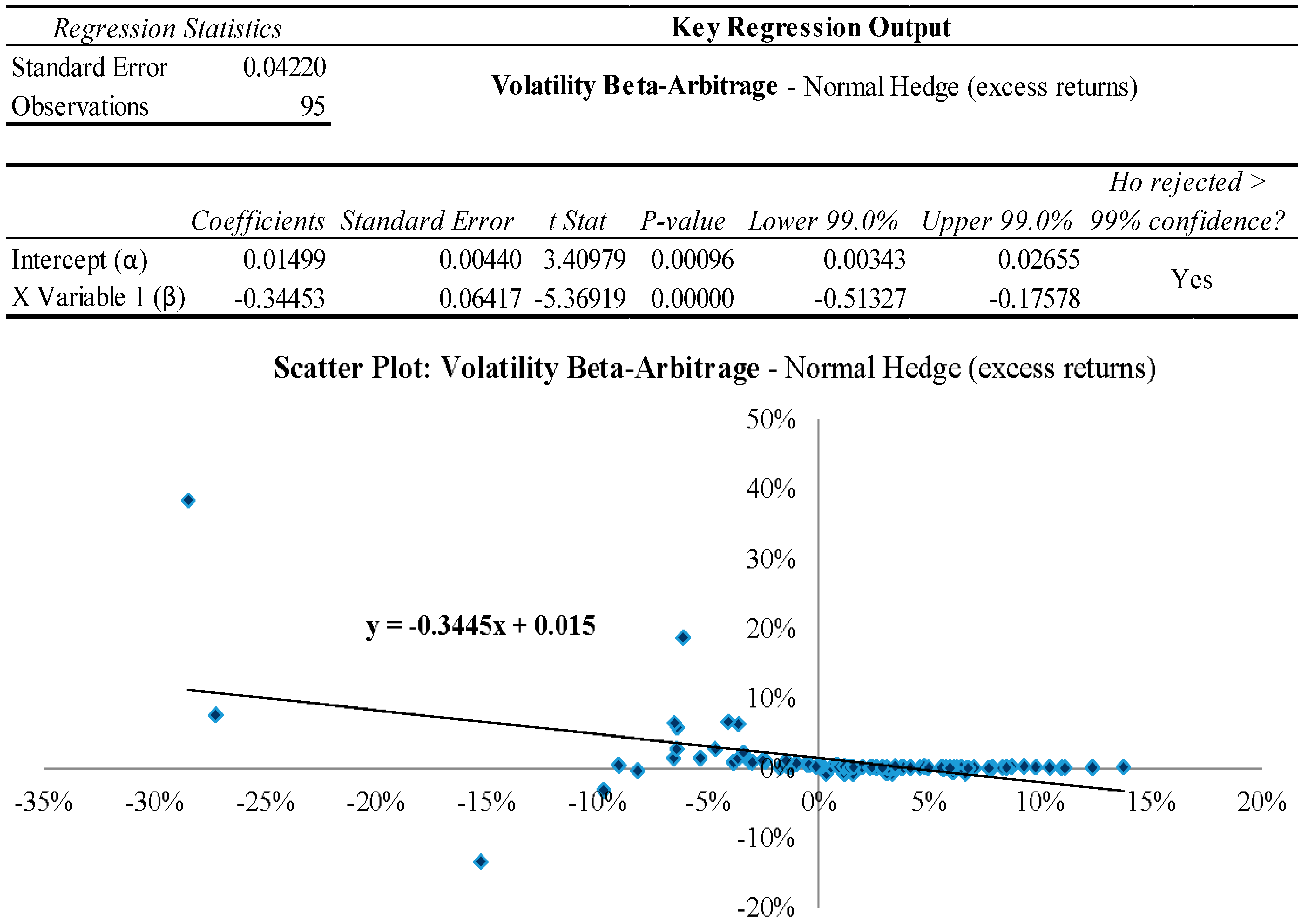

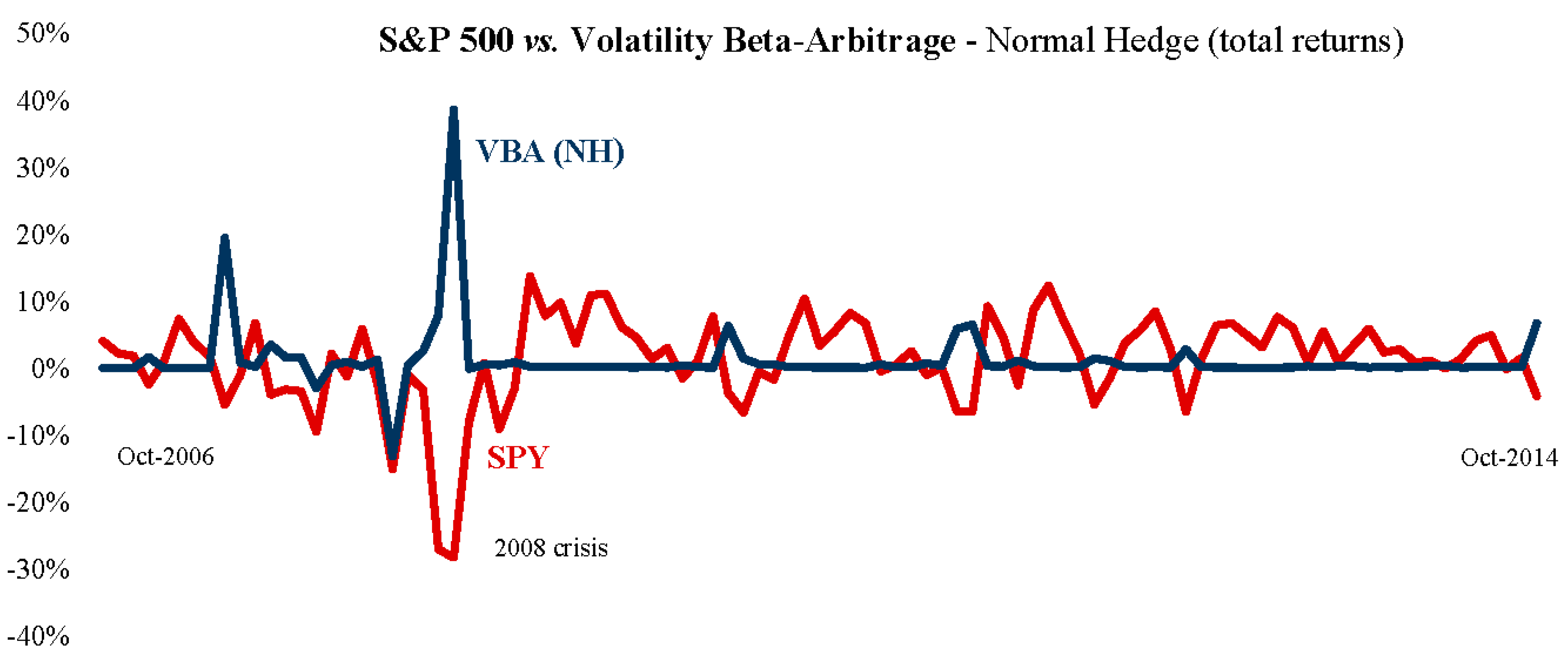
Figure A2.
Note how the strategy gives a general counteraction to the dips in the benchmark, right up until the latest dip in 2014.
Figure A2.
Note how the strategy gives a general counteraction to the dips in the benchmark, right up until the latest dip in 2014.
Appendix B. Tail Hedge, October 2006–October 2014
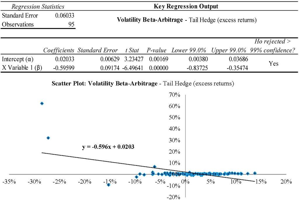
Figure A3.
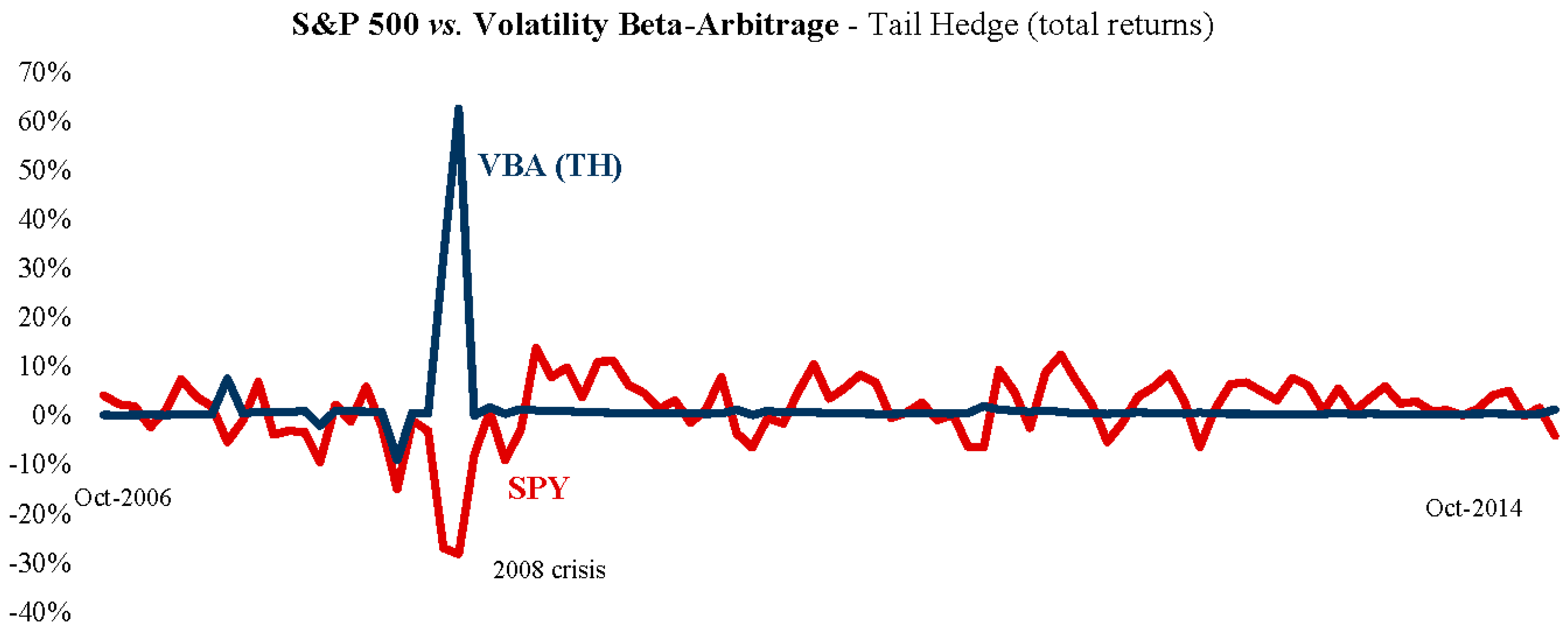
Note how, with this strategy, the counteraction to systematic risk is even more attractive in the sell off of 2008.
Figure A3.
Note how, with this strategy, the counteraction to systematic risk is even more attractive in the sell off of 2008.


Figure A4.
Another visualization of an even greater counter to the 2008 crisis.
Figure A4.
Another visualization of an even greater counter to the 2008 crisis.
Appendix C. Triple Leveraged, Normal Hedge, October 2010–October 2014

Figure A5.
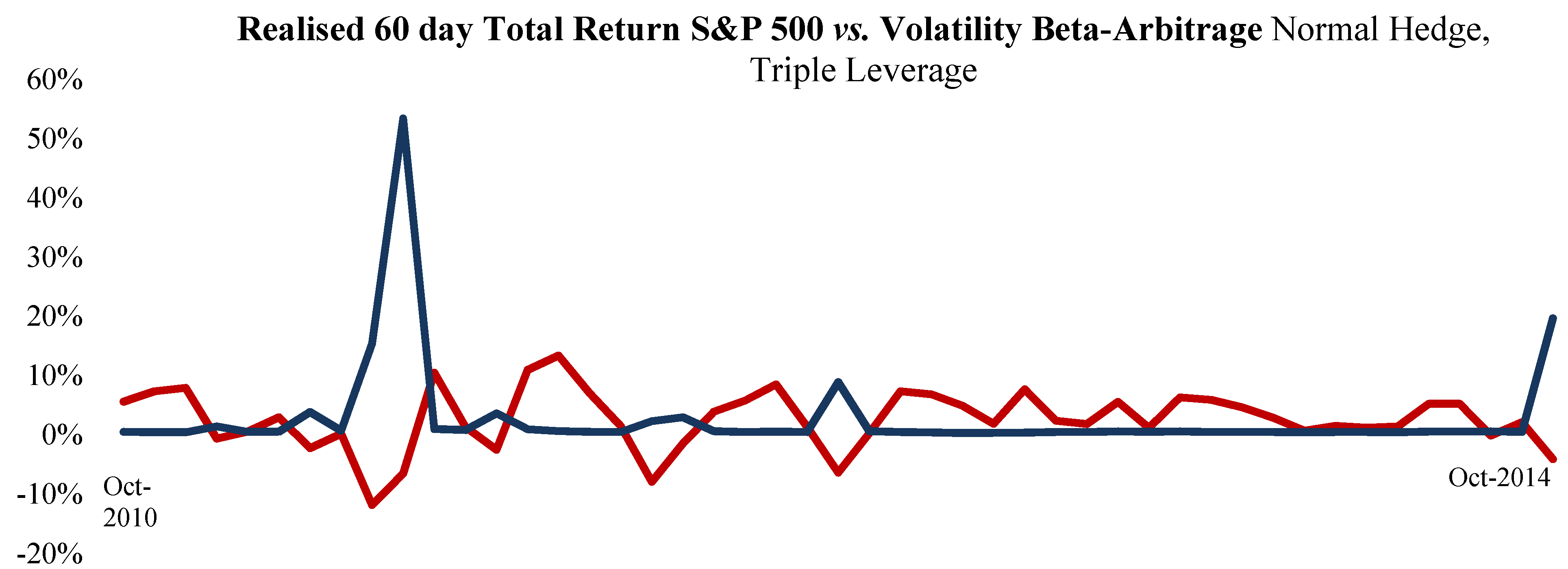
The previous two charts may have instilled doubt of whether the counteraction was specific to the 2008 crisis, the increased leverage with this strategy, show that the same counteraction to systematic risk applies even when the magnitude of the moves were reduced over the more bullish period.
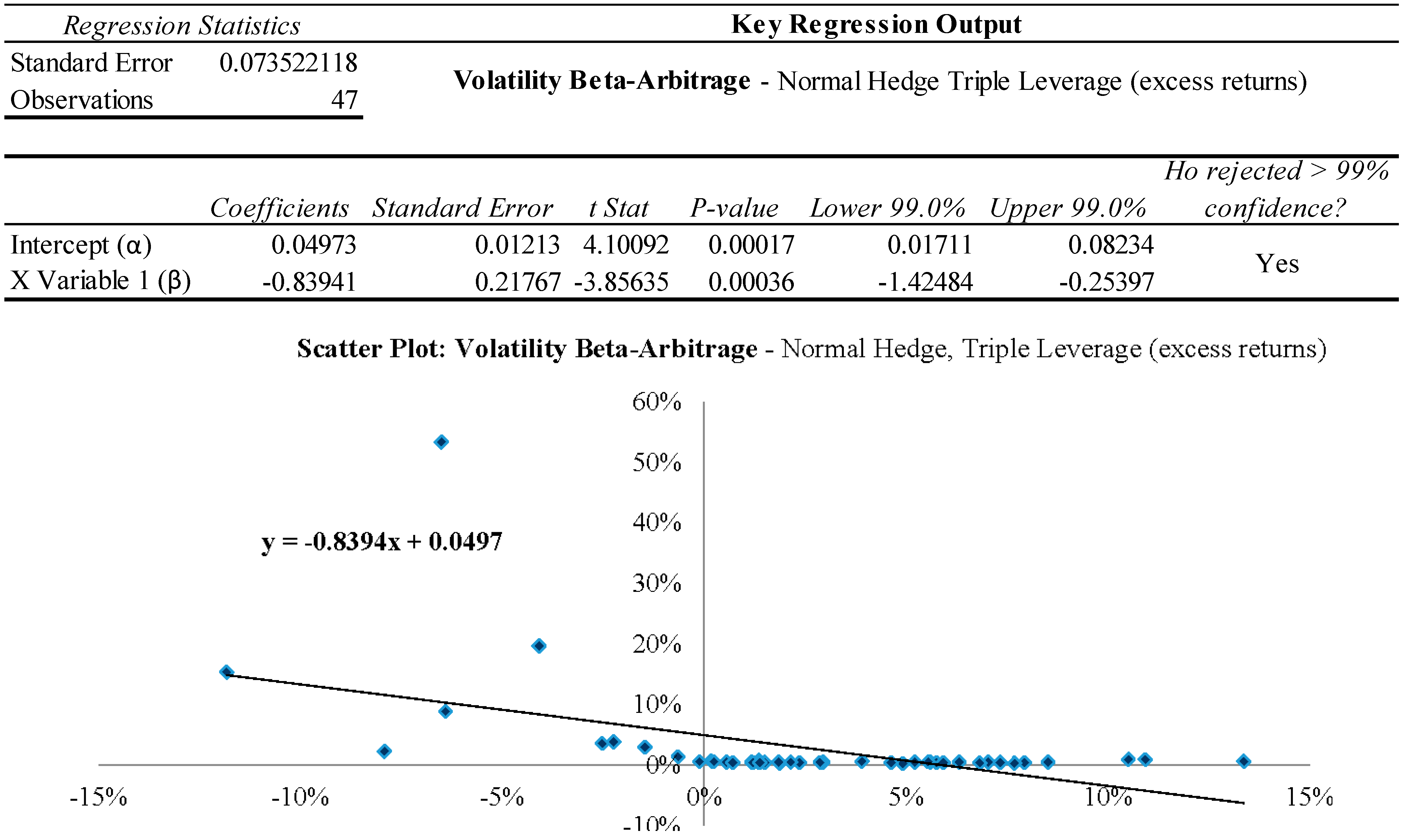

Figure A6.
The chart shows the realized returns with the increased leverage.
Figure A6.
The chart shows the realized returns with the increased leverage.
Appendix D. The Daily Performance Progression of the Strategies
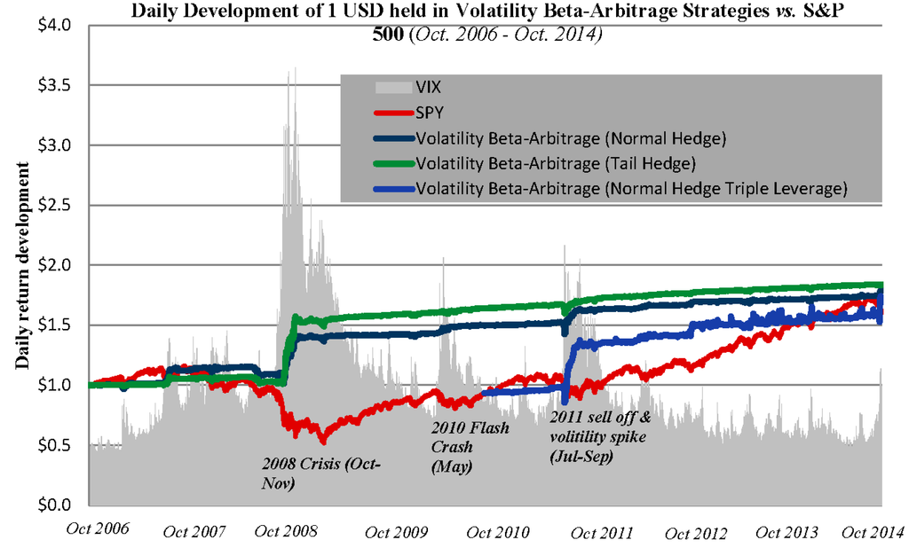
Figure A7.
The above chart gives a visualization of the compounded development for all of the strategies against the benchmark (SPY), accounting for slippage and transaction costs. Note the low volatility of returns and how the strategies are “long” the VIX as they rise with sudden up moves in this index (represented in grey).

Appendix E. Out of Sample Tests

Figure A8.
This chart shows the bimonthly returns, of the strategy vs. the benchmark, in the subsequent 10 months after the original study was performed. What we see is that the Normal Hedge strategy appears to still be performing in a similar manner to the original study as a counter to systematic risk.
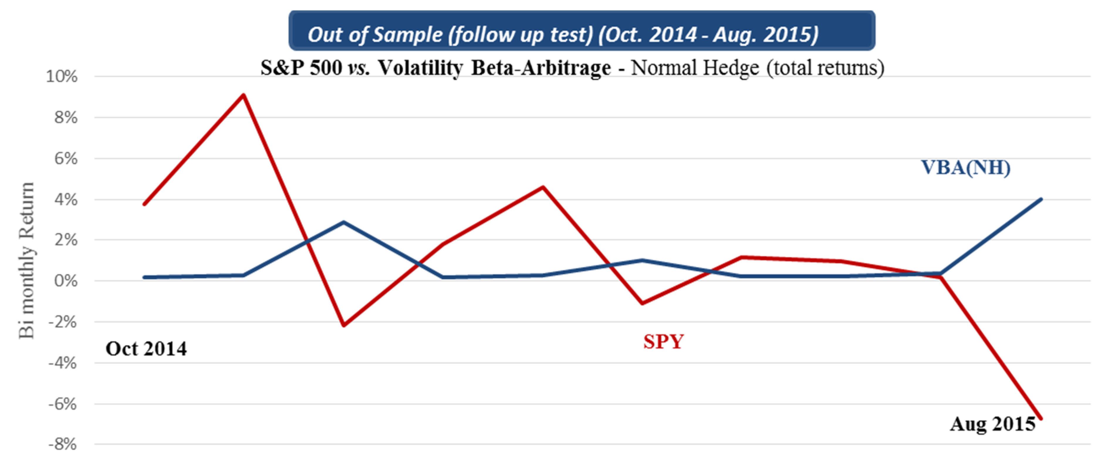
The out of sample tests listed in individual charts (showing bimonthly performance) and in a combined chart (showing daily performance) illustrate the continued performance of the strategies after the initial analysis. The reason for following up on the development of the strategies is to examine whether performance has deteriorated since we identified these possible opportunities. As can be seen, they continue to display characteristics very similar to that of the initial study.

Figure A9.
The Tail Hedge strategy, again appears to be robust in the out of sample test, less sensitive to the dips in the benchmark than the Normal Hedge but overall still performing in the same manner towards systematic risk as the original study.
Figure A9.
The Tail Hedge strategy, again appears to be robust in the out of sample test, less sensitive to the dips in the benchmark than the Normal Hedge but overall still performing in the same manner towards systematic risk as the original study.
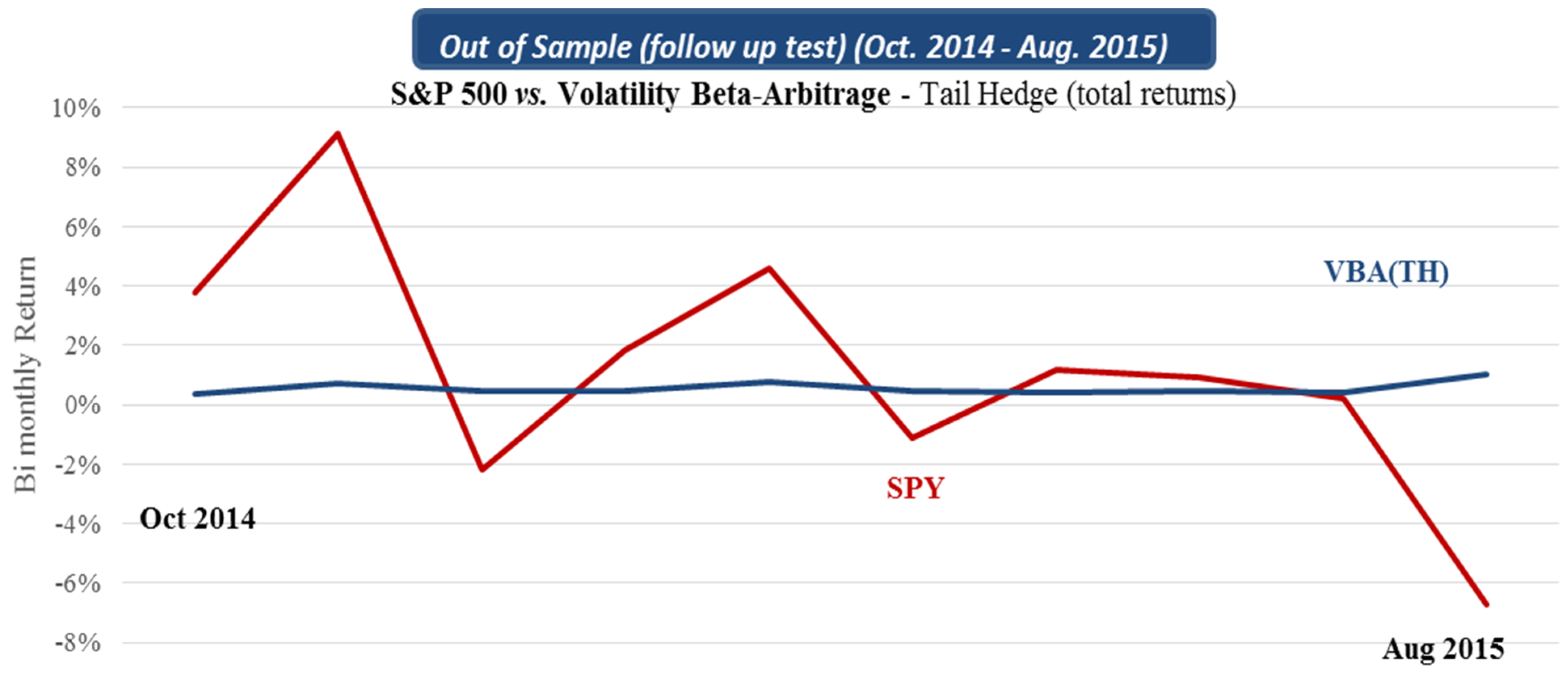

Figure A10.
This chart shows that the Triple Leverage strategy also worked very well in the out of sample period against systematic risk in the market.
Figure A10.
This chart shows that the Triple Leverage strategy also worked very well in the out of sample period against systematic risk in the market.
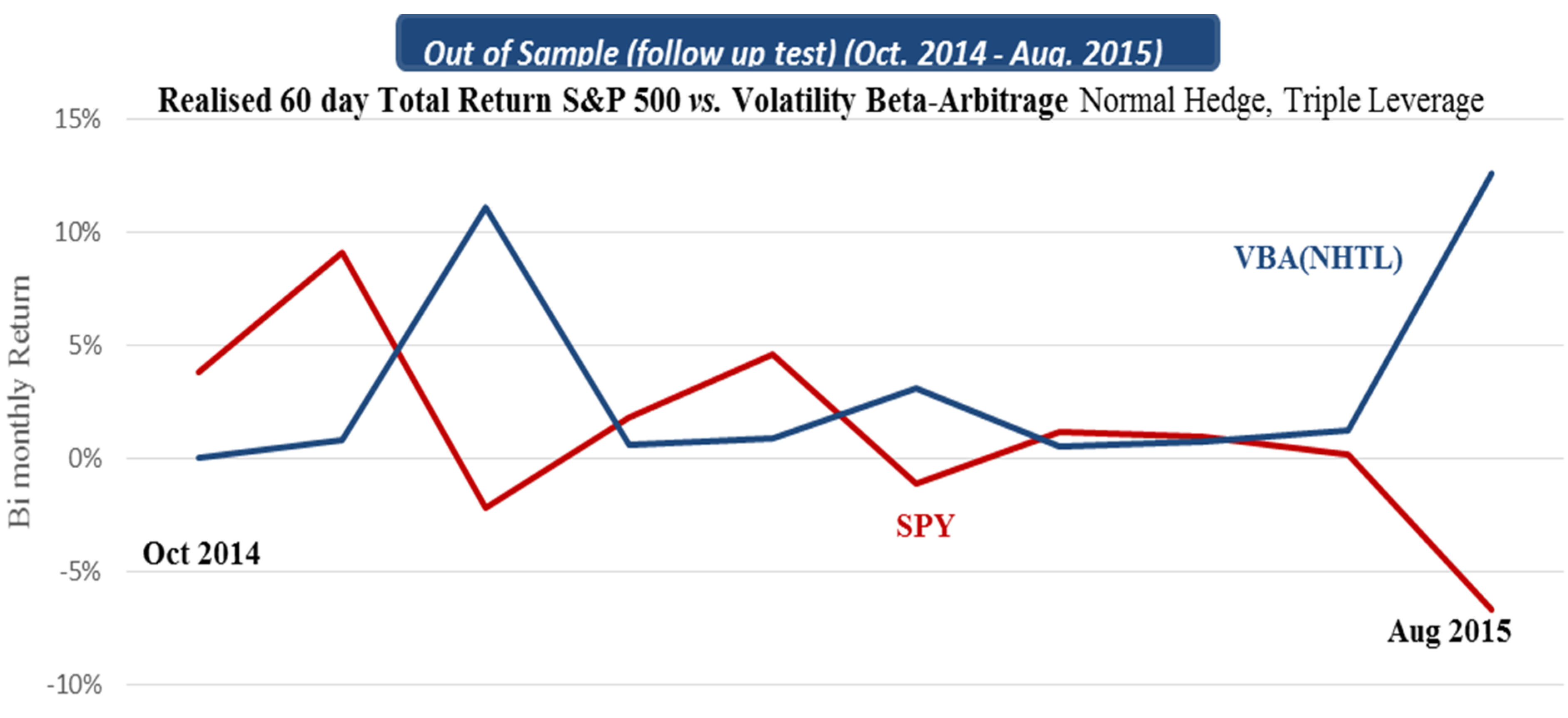

Figure A11.
This chart shows the same return development as in Appendix D, but with the continued development of the out of sample test (October 2014 to August 2015).
Figure A11.
This chart shows the same return development as in Appendix D, but with the continued development of the out of sample test (October 2014 to August 2015).
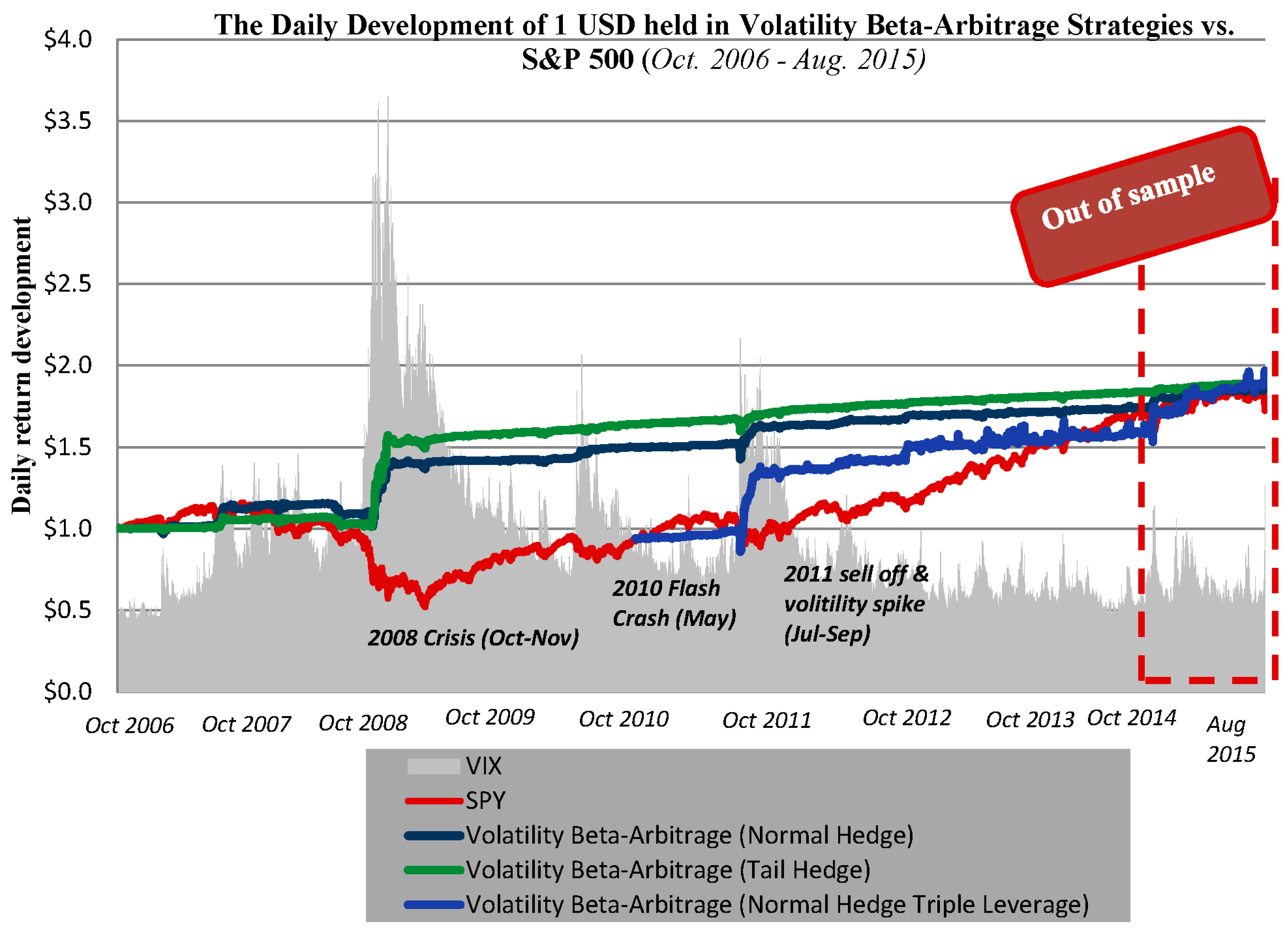
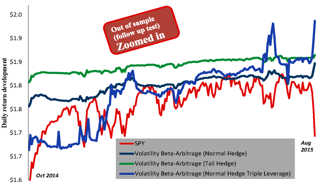
Figure A12.
This chart shows the daily development of the strategies against the benchmark for the out of sample test, and, as can be seen, even on a daily basis, all of the strategies continue to function as generally effective counters to systematic risk, especially in the late August selloff.
Figure A12.
This chart shows the daily development of the strategies against the benchmark for the out of sample test, and, as can be seen, even on a daily basis, all of the strategies continue to function as generally effective counters to systematic risk, especially in the late August selloff.

References
- R. Dobbs, S. Lund, J. Woetzel, and M. Mutafchieva. “Debt and (Not Much) Deleveraging.” Available online: http://www.mckinsey.com/insights/economic_studies/debt_and_not_much_deleveraging (accessed on 1 March 2015).
- I. Badshah. “Asymmetric Return-Volatility Relation, Volatility Transmission and Implied Volatility Indexes.” SSRN Electron. J., 2009. [Google Scholar] [CrossRef]
- A. Chandra, and M. Thenmozhi. “On asymmetric relationship of India volatility index (India VIX) with stock market return and risk management.” Off. J. Indian Inst. Manag. Calcutta 42 (2014): 33–55. [Google Scholar] [CrossRef]
- S. Dash, and M.T. Moran. “VIX as a Companion for Hedge Fund Portfolios.” J. Altern. Invest. 8 (2005): 75–80. [Google Scholar] [CrossRef]
- A.M. Hibbert, R.T. Daigler, and B. Dupoyet. “A behavioural explanation for the negative asymmetric return-volatility relation.” J. Bank. Financ. 32 (2008): 2254–2266. [Google Scholar] [CrossRef]
- J.C. Jackwerth. “Recovering Risk Aversion from Option Prices and Realised Returns.” Rev. Financ. Stud. 12 (2000): 433–451. [Google Scholar] [CrossRef]
- E. Szado. “VIX Futures and Options: A Case Study of portfolio Diversification During the 2008 Financial Crisis.” J. Altern. Invest. 12 (2009): 68–85. [Google Scholar] [CrossRef]
- R.H. Thaler, and E.J. Johnson. “Gambling with the House Money and Trying to Break Even: The Effects of Prior Outcomes on Risky Choice.” Manag. Sci. 36 (1990): 644–660. [Google Scholar] [CrossRef]
- R.J. Shiller. “Preference to the Second.” In Irrational Exuberance Revised and Expanded, 3rd ed. Princeton, NJ, USA: Princeton University Press, 2015. [Google Scholar]
- “Shiller P/E Ratio for the S&P 500.” Available online: http://www.multpl.com/shiller-pe/ (accessed on 3 March 2015).
- D. Kahneman, and A. Tversky. “Prospect Theory: An Analysis of Decision under Risk.” Econometrica 47 (1979): 263–291. [Google Scholar] [CrossRef]
- A. Tversky, and D. Kahneman. “Judgment under Uncertainty: Heuristics and Biases.” Science 185 (1974): 1124–1131. [Google Scholar] [CrossRef] [PubMed]
- 1.Szado [7] noted that the extra leverage provided by deep OTM VIX calls resulted in greater return benefits than SPX/SPY puts in market declines.
- 2.VIX options have parity to the VIX futures of the same expiration date, which is why it is important to use the relevant futures prices as the underlying asset and not the spot VIX index itself (as the VIX cannot be directly traded).
- 3.This parameter tells us, given the value of the respective SPY put and volatility calls, how many volatility calls are needed when initiating a position.
- 4.This parameter expresses the credit to be received as a percentage of the value of the options purchased [Sz + Vz·Kz] in the position.
- 5.Margin Considerations: Since option selling holds risk, an individual or institution needs to put down a certain amount of collateral (usually in the form of cash) to hold a short option position open (margin). Among other possible factors, the amount of margin required can depend on, (1) the calculated risk of the position; (2) government regulations; (3) overall account risk; (4) credit status of individuals or institutions; and (5) account types. This means that the capital requirements for the proposed strategies can differ depending on who is using them and therefore that their implementation may be more/less attractive to some parties than to others.
- 6.The Sharpe ratio, which accounts for the return, over the standard deviation of the strategy, uses daily return data of the compounded portfolios. This insures a risk return measure that is inclusive of Greek risks inherent in options strategies.
© 2015 by the authors; licensee MDPI, Basel, Switzerland. This article is an open access article distributed under the terms and conditions of the Creative Commons Attribution license (http://creativecommons.org/licenses/by/4.0/).
