Article

Convergence Studies on Monte Carlo Methods for Pricing Mortgage-Backed Securities

1
Department of Mathematics, North Carolina State University, Raleigh, NC 27695-8205, USA
2
Department of Mathematics, University of Houston-Clear Lake, 2700 Bay Area Blvd., Houston, TX 77058, USA
3
ZM Financial Systems, 5915 Farrington Road, Unit 201, Chapel Hill, NC 27517, USA
*
Author to whom correspondence should be addressed.
Int. J. Financial Stud. 2015, 3(2), 136-150; https://doi.org/10.3390/ijfs3020136
Submission received: 16 February 2015 / Revised: 22 April 2015 / Accepted: 24 April 2015 / Published: 5 May 2015

Abstract

:
Monte Carlo methods are widely-used simulation tools for market practitioners from trading to risk management. When pricing complex instruments, like mortgage-backed securities (MBS), strong path-dependency and high dimensionality make the Monte Carlo method the most suitable, if not the only, numerical method. In practice, while simulation processes in option-adjusted valuation can be relatively easy to implement, it is a well-known challenge that the convergence and the desired accuracy can only be achieved at the cost of lengthy computational times. In this paper, we study the convergence of Monte Carlo methods in calculating the option-adjusted spread (OAS), effective duration (DUR) and effective convexity (CNVX) of MBS instruments. We further define two new concepts, absolute convergence and relative convergence, and show that while the convergence of OAS requires thousands of simulation paths (absolute convergence), only hundreds of paths may be needed to obtain the desired accuracy for effective duration and effective convexity (relative convergence). These results suggest that practitioners can reduce the computational time substantially without sacrificing simulation accuracy.

1. Introduction

From trading to risk management, Monte Carlo methods are widely used in pricing MBS instruments. A successful implementation of a Monte Carlo method should be able to calculate the full risk profile of an MBS instrument in addition to its price. More details about the Monte Carlo method can be found in Glasserman [1]. In many situations, it is the risk profile, not the price, that is the focus of most practitioners.
In order to obtain the risk profile of an MBS instrument, one first needs to be able to price the MBS instrument. Under certain market environments, one can calculate the implied option-adjusted spread (OAS) at a given market price. Using the calculated OAS, one can then calculate the prices of the MBS instrument under different interest rates and volatility scenarios. These prices allow the Greeks to be calculated numerically. For example, we can calculate prices with interest rates shifting up and down and, therefore, obtain the effective duration (DUR) and the effective convexity (CNVX), which are the first and second derivatives of the price to the interest rates, respectively. For more information about MBS, OAS, DUR and CNVX, we refer readers to Fabozzi [2].
In this process, it is very natural to obtain OAS with desired accuracy first and to calculate the Greeks using OAS afterwards. Unfortunately, given the high dimensionality and slow convergence of MBS instruments, using the Monte Carlo method to price a MBS instrument is generally time consuming. It is not unusual that it requires tens of thousands of simulation paths before the convergence of the OAS of a MBS instrument can be reached. On the other hand, for many practitioners, the goal is to find the associated Greeks and to obtain the risk profile of an MBS instrument. OAS is merely an intermediate vehicle in this practice. We know that the value of OAS and its convergence depend on the selection of stochastic models, random number generators, as well as the number of paths. However, should we expect the same for the Greeks like DUR and the CNVX? This is the question answered by this paper.
This paper is organized as the follows. In Section 2, we introduce the concept of the coefficient of variation (CV) to measure the rate of the convergence. We define two types of convergence—absolute convergence and relative convergence—and we show that it is mathematically feasible to establish relative convergence without absolute convergence. In Section 3, we describe our pricing methodology, as well as model selections and parameters. In Section 4, the numerical results of OAS, DUR and CNVX for a selection of MBS instruments and our analysis of the results are presented. We conclude our findings in Section 5.

2. Absolute Convergence and Relative Convergence

In this section, we will give a way to measure the speed of convergence of estimators of OAS, DUR and CNVX. Then, we will give the definition of relative convergence and absolute convergence. In addition, we explore the feasibility of the relative convergence mathematically.

2.1. Measure of Convergence: Coefficient of Variation

Because we are going to look at the rate of convergence of the random estimators of OAS, DUR and CNVX, we need to specify how to measure the rate of convergence.
Usually, if we have two non-biased statistical estimators μ ^ 1 and μ ^ 2 for a variable μ, we only need to compare the standard variations of μ ^ 1 and μ ^ 2 . The smaller the standard deviation is, the better the estimator is. When we use Monte Carlo simulations, for a given number of paths, we can compare the standard deviations to determine which estimator converges faster than the other.
However, in our situation here, we need to estimate three quantities, OAS and two Greeks, DUR and CNVX. The mean value of the OAS and those two Greeks may be significantly different from each other. Therefore, a similar standard deviation may not mean the same degree of dispersion for the estimators of OAS, DUR and CNVX. For example, a standard deviation of five for a normal distribution with a sample mean of 1000 will give us a 95% confidence interval of [ 990 , 1010 ] , only a 1% fluctuation around its sample mean value. However, a standard variation of five for a normal distribution with sample mean 10 will only give us a 95% confidence interval of [ 0 , 20 ] , a 100% fluctuation around its sample mean value. Therefore, using their standard deviation directly to compare the rates of convergence will not make much sense.
In order to solve this issue, we normalize the standard deviations by virtue of their sample means. Here, we use the coefficient of variation (CV), which is defined as:
c v = σ ^ μ ^
where σ ^ is the sample standard variation and μ ^ is the sample mean. The CV is a normalized measure of the dispersion of a probability distribution.
For a given number of paths, we will calculate the CV’s for the estimators of OAS, DUR and CNVX. The smaller CV means a better estimator; therefore, it implies a faster convergence.

2.2. Absolute Convergence and Relative Convergence

To describe the connection between the convergence of OAS and DUR/CNVX, here, we define two types of convergence: absolute convergence and relative convergence for Monte Carlo simulations. As we mentioned earlier, to obtain DUR/CNVX, we need to obtain OAS first. For a given degree of accuracy, such as a given CV, if both OAS and DUR/CNVX reach the desired accuracy, we call this absolute convergence. Quantitatively, the absolute convergence is measured by the number of paths needed for both OAS and DUR/CNVX to reach the desired CV, which is called the degree of the absolute convergence. On the other hand, for the relative convergence, we only look at the convergence of DUR/CNVX, regardless of the convergence of OAS, the intermediate vehicle. In other words, for a given degree of accuracy (CV), when the estimators of DUR/CNVX reach the desired accuracy, no matter how OAS converges, we call it the relative convergence. Quantitatively, the relative convergence can be measured with the number of paths for DUR/CNVX to converge or to reach the desired CV, which is called the degree of relative convergence for the given CV.
For a given CV, if the degree of absolute convergence is large than that of the relative convergence, the number of paths needed to reach the absolute convergence is larger than that to reach the relative convergence. In other words, a longer computation time is needed when we seek absolution convergence. In the mean time, to obtain DUR/CNVX with desired accuracy, we can seek relative convergence instead of absolute convergence in order to save computational time.
In our paper, we found that for MBS instruments, the degree of absolute convergence is much larger than the degree of relative convergence, for a given desired accuracy. Actually, according to our results, by seeking the relative convergence instead of the absolute convergence, we can save computational time by 50% to 99%.

2.3. Mathematical Feasibility

Let us give a simple example to illustrate why the relative convergence is possible. Assume that X is a normal random variable with mean μ and variance σ 2 . We consider a function of X, Y = f ( X ) = X 2 , and its derivative function, Z = f ( X ) = 2 X . If we use Monte Carlo simulation to estimate E [ Y ] and E [ Z ] , we can use the following non-bias estimators:
Y ^ X 1 2 + X 2 2 + + X N 2 N
Z ^ 2 X 1 + 2 X 2 + + 2 X N N
where X 1 , X 2 , X N are i.i.d. r.v.with the same distribution of X.
Now, for a given number of simulations, N, we calculate the rate of convergence in terms of CV. For the estimator Y ^ , we can get:
c v ( Y ^ ) = σ ( Y ^ ) E [ Y ^ ] = V a r ( X 2 ) N E [ X 2 ] = E [ X 4 ] - ( E [ X 2 ] ) 2 N E [ X 2 ] = μ 4 + 6 μ 2 σ 2 + 3 σ 4 - ( μ 2 + σ 2 ) 2 N ( μ 2 + σ 2 ) = σ 4 μ 2 + 2 σ 2 N ( μ 2 + σ 2 )
On the other hand, for the estimator Z ^ , we have:
c v ( Z ^ ) = σ ( Z ^ ) E [ Z ^ ] = V a r ( 2 X ) N E [ 2 X ] = σ μ N
From the above results, we can see that if σ 4 μ 2 + 2 σ 2 N ( μ 2 + σ 2 ) > σ μ N or, equivalently, μ > σ 5 - 1 4 , the CV of the estimator Z ^ will be smaller than the CV of the estimator Y ^ . In other words, for a given CV, the number of simulations required for the estimator Z ^ to reach the desired CV will usually be less than that for the estimator Y ^ . This means that the convergence of the estimator Z ^ is faster than that of the estimator Y ^ .
Of course, the situation for OAS and the DUR/CNVX of MBS instruments is much more complicated than the example given above. However, as the example indicated, it is possible that the convergence speed of DUR/CNVX is faster than the convergence speed of OAS. That being said, if the values of DUR/CNVX are the final goals of the simulation, we can reach the desired accuracy for a relatively small number of paths, even though OAS may not be very close to its real value.
Our main result in this paper is that relative convergence does exist for MBS and MBS derivatives. In other words, to achieve the desired accuracy of DUR/CNVX, it is not necessary to achieve very good accuracy for OAS first. The error of OAS does not have too much influence on DUR/CNVX. Usually, more than 10 4 interest rate paths are needed to see the convergence of OAS. However, according to our study, only hundreds of paths are needed to see the convergence of DUR/CNVX, even though we use the not-so-accurate OAS as our input in the computation of DUR/CNVX. Given this result, practitioners can save computational time significantly.

3. Pricing Methodology and Model Selection

To price an MBS instrument using Monte Carlo simulation, we first need to specify an interest rate model and a prepayment model. For every interest rate path, the prepayment speeds, the cash flow and, therefore, the price will be calculated. By taking average of the prices of many randomly-generated interest rate paths, we can obtain the price of the MBS instrument. For more information about the MBS pricing and Monte Carlo simulations, we refer readers to Fabozzi [2], Caflisch, Morokoff and Owen [3], Richard and Roll [4], Glasserman [1] and the references therein.

3.1. Pricing Methodology

Once we know how to price an MBS instrument using a particular interest rate model, we can calculate its DUR and CNVX. In particular, to calculate effective duration and CNVX, the following six-step valuation procedure is used:
  • Calibrate interest rate and volatility term structures to the market yield curves (Treasury, LIBOR and Swap), and interest rate derivatives (Caps, Floors and Swaptions).
  • Generate stochastic interest rate paths using calibrated interest rate and the volatility term structure.
  • Generate cash flows for the MBS for each stochastic path.
  • Calculate prices for each stochastic path. By the strong law of large numbers, the MBS price is given by:
    V = lim N 1 N i = 1 N V i
  • Iterate Step 1 to Step 4 by changing OAS until the calculated price equals the market price.
  • Apply the calculated OAS to obtain prices for interest rates up and down 100 basis points, and DUR and CNVX are given by:
    DUR = V - - V + 2 V 0 Δ y
    CNVX = V - + V + - 2 V 0 V 0 ( Δ y ) 2
    where V 0 , V - , V + are the prices of the underlying MBS bond when the interest rates are current, down by 100 basis points and up by 100 basis points, respectively. In addition, Δ y = 100 basis points.
In this study, we use the Black–Karasinski interest rate model proposed in [5]:
d ln r t = θ [ a - ln r t ] d t + σ d w t
where θ , a , σ are constants and w t is a standard Brownian motion. This is a very popular interest rate generating procedure with mean reversion θ = 0 . 005 .
Simulation results of this paper are generated using the MBS pricing engine of ZMFinancial Systems’ Asset Liability Management (ALM) model. The ZM Financial Systems’ proprietary prepayment model is used to project prepayment speeds on each stochastic path. The market data used are as of the market close of 6 December 2007.

3.2. Pseudo-Random Number Generators

Computers cannot generate real random numbers, because they generate numbers in a deterministic fashion based on some arithmetic algorithms. If the computer sequence has no or tolerable correlation, then this computer-generated sequence is called pseudo-random.
There are several widely-used random number generators to generate uniform distributions over [ 0 , 1 ] . The NR1 (Ran1) in [6] is the usual linear congruent generator with the minimal standard presented by Park and Miller [7]. It was found that this algorithm has a period around of 10 9 . Later, NR2 (Ran2) [6] was often used, which has a period of more than 10 18 . NR3 (Ran3) [6] is a subtractive method with a portable routine [8,9]. Mersenne twister (MT) is a very recently developed pseudo-random number generator (see Matsumoto and Nishimura [10]). It is based on a matrix recurrence over a finite binary field F 2 , which provides for fast generation of very high quality pseudo-random numbers. Its period can be as large as 2 19937 - 1 , and it has a very high order of dimensional equi-distribution.
In this paper, we will use Ran3 (NR3) and MT as our random number generators. Numerical experiments using Ran1 and Ran2 gave us similar results to the results using Ran3, so we omit Ran1 and Ran2 here.
Those generators are used to generate random numbers that are uniformly distributed over [ 0 , 1 ] . To convert these pseudo-uniform random numbers into pseudo-normal random numbers, we consider two methods, namely Box–Müller (BM) [6] and inverse cumulative distribution function (INV).
To test the robustness of our method, we consider the combinations of two random number generators, NR3 and MT, and two methods to convert uniform random variables into normal random variables, BM and INV. The combinations are referred to as NR3-INV, NR3-BM, MT-INV and MT-BM.

3.3. Convergence Analysis

In this paper, we report the numerical results (see Section 4) for a representative selection of three MBS instruments. These are:
  • A planned amortization class (PAC) bond (CUSIP: 31396UY46);
  • A Support (CUSIP: 31397HLJ5, “Support”);
  • A pass-through MBS bond (FNCL6.0).
In order to test the convergence of the random estimators for OAS and DUR/CNVX, we consider eight random seeds in each pricing process:
A s = { - 26 , 810 , - 6 , 108 , - 30 , 650 , - 90 , 254 , - 66 , 368 , - 50 , 401 , - 97 , 973 , - 36 , 457 }
which are generated using the random number generator in MS-Excel.
We first use Monte Carlo simulations to price the OAS of the three selected MBS instruments with those eight initial random seeds. Then, based on OAS obtained, we compute the DUR and the CNVX of the MBS instruments. These results about DUR and CNVX are very important, as they tell us how the MBS prices change as the interest rates change.
For any given number of paths, we navigate the speed of convergence for all scenarios by virtue of the coefficient of variation defined earlier. More particular, for a given number of paths, n, we use the Monte Carlo method and the eight difference random seeds mentioned above to obtain eight values for an estimator P n s , s A s , which can be the estimator for OAS, DUR or CNVX. Then, using the eight values obtained, the standard variation for the given number of paths will be calculated in the following way:
σ ^ n = 1 7 s A s ( P n s - P ^ n ) 2
where:
P ^ n = 1 8 s A s P n s
Given the sample standard variation σ ^ n and the sample mean P ^ n , we can calculate the CV for the given number of paths:
c v ( P ^ n ) = σ ^ n P ^ n
For each pricing process, we consider the following numbers of paths:
A p = { 50 , 100 , 200 , 300 , , 1 , 000 , 2 , 000 , 3 , 000 , , 10 , 000 }
For any of the given number of paths, we will calculate the CVs of OAS, DUR and CNVX for the selected MBS instruments. By comparing their CVs, we can determine the degree of convergence for those three variables.
This procedure will be repeated for all three market-traded securities, the PAC, the Support and the FNCL, and for all four pseudo-random number generators, MT-BM, MT-INV, NR3-BM and NR3-INV. The numerical results and analysis will be given next.

4. Numerical Results and Analysis

In this section, we present the numerical results about the convergence behaviors of the OAS, the DUR and the CNVX of the three selected MBS instruments. For each selected MBS instrument, we compare the convergence of OAS, DUR and CNVX using different random number generator combinations. We find that for all scenarios, the degree of absolute convergence is larger than the degree of relative convergence for all three MBS instruments. Therefore, by seeking relative convergence instead of absolute convergence, we can save computational time. Details will be given in the following parts.

4.1. Convergence of OAS

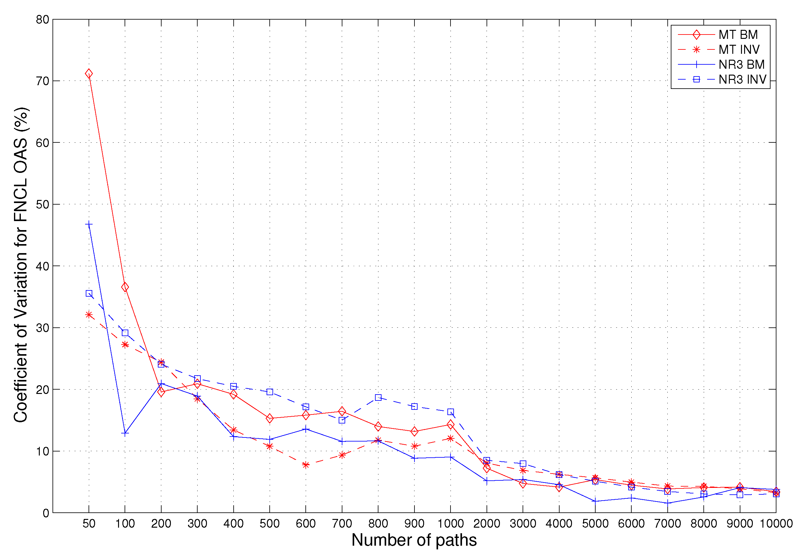
For the three MBS instruments we consider, we calculate the CV of the OAS using four random number generator combinations, MT-BM, MT-INV, NR3-BM and NR3-INV. We give the numerical results for FNCL, which are shown in Figure 1. The convergence pattern for PAC and Support are very similar, and we omit them here.
Figure 1. The convergence of OAS for the FNCL. The vertical axis is for the coefficient of variation (%). The horizontal axis is the number of paths.
Ijfs 03 00136 g001
As we can see from the figure, for all four random number generators, OAS does show the convergence properties, and the convergence patterns are very similar to each other. On the other hand, we can tell from the graph that, to reach an accuracy with a CV of 5%, we need about 4,000–6,000 paths. For 10,000 paths, the CVs are about 3% for all four random generators. In other words, the convergence of the OAS of FNCL is not very fast.
Next, we will look at the convergence behaviors of DUR, effective duration, and CNVX, effective convexity of FNCL.

4.2. The Effective Duration and the Effective Convexity

Using OAS obtained by calibrating to the market prices of any selected MBS instrument, we can price the MBS instrument with the interest rate shifting up or down by 100 basis points. Then, by virtue of Equations (6) and (7), we can evaluate the DUR and the CNVX of the MBS instrument, which describe the sensitivity of the MBS price against the changes in interest rate. This will also help determine where the value goes and where the risk goes in the MBS structure.
DUR measures the price sensitivity of the MBS with respect to the changes of interest rates. It can be described by the first derivative of the MBS price w.r.t. interest change. CNVX is the second derivative of the MBS price w.r.t. the interest rate change. It measures the sensitivity of DUR to the changes of the interest rate.
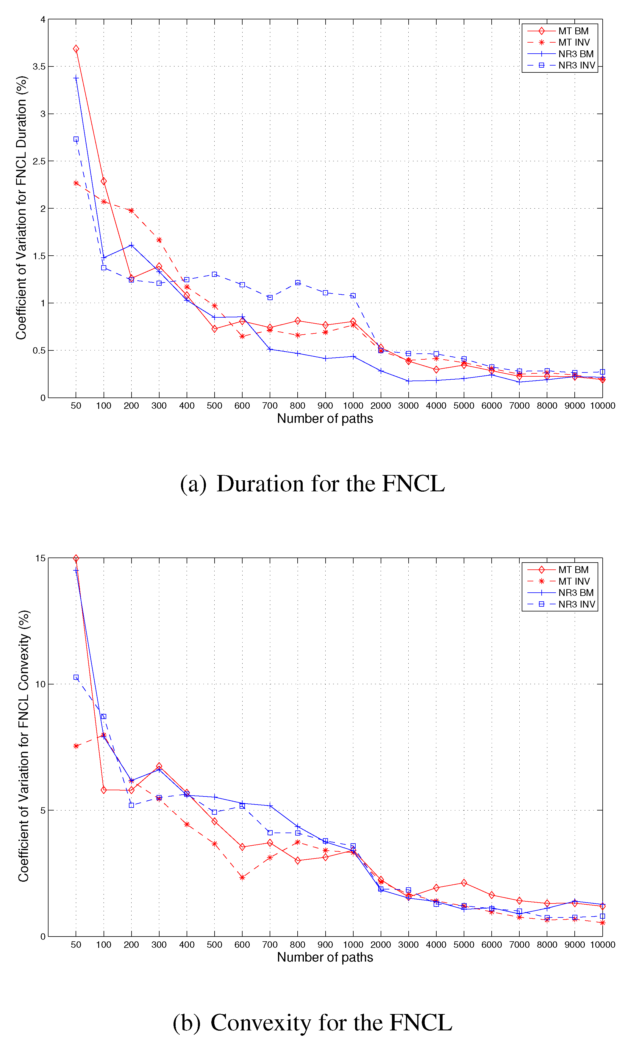
The convergence behaviors of DUR and CNVX for FNCL using the four different random number generators are given in Figure 2.
Figure 2. The Convergence of DUR and CNVX of the FNCL. The vertical axis is for the coefficient of variation (%). The horizontal axis is the number of paths.
Ijfs 03 00136 g002
As we can tell from the figure, both DUR and CNVX show the convergence property for different random number generators, and the patterns are very similar for different random number generators. On the other hand, we can see that the convergence speeds of DUR and CNVX are faster than that of OAS. For example, if we use 6000 paths, the CV of OAS is only 5%, for which the CV for DUR is about 0.4% and the CV for CNVX is about 1.5% for all random number generators. We will compare their convergence speeds in the next subsection.
In addition, we ran the same numerical experiments for the PAC and the Support, too. The numerical results are similar to that of the FNCL. There are some minor difference. We will present the numerical results later in Subsection 4.4, the robustness test part.

4.3. Relative Convergence and Absolute Convergence

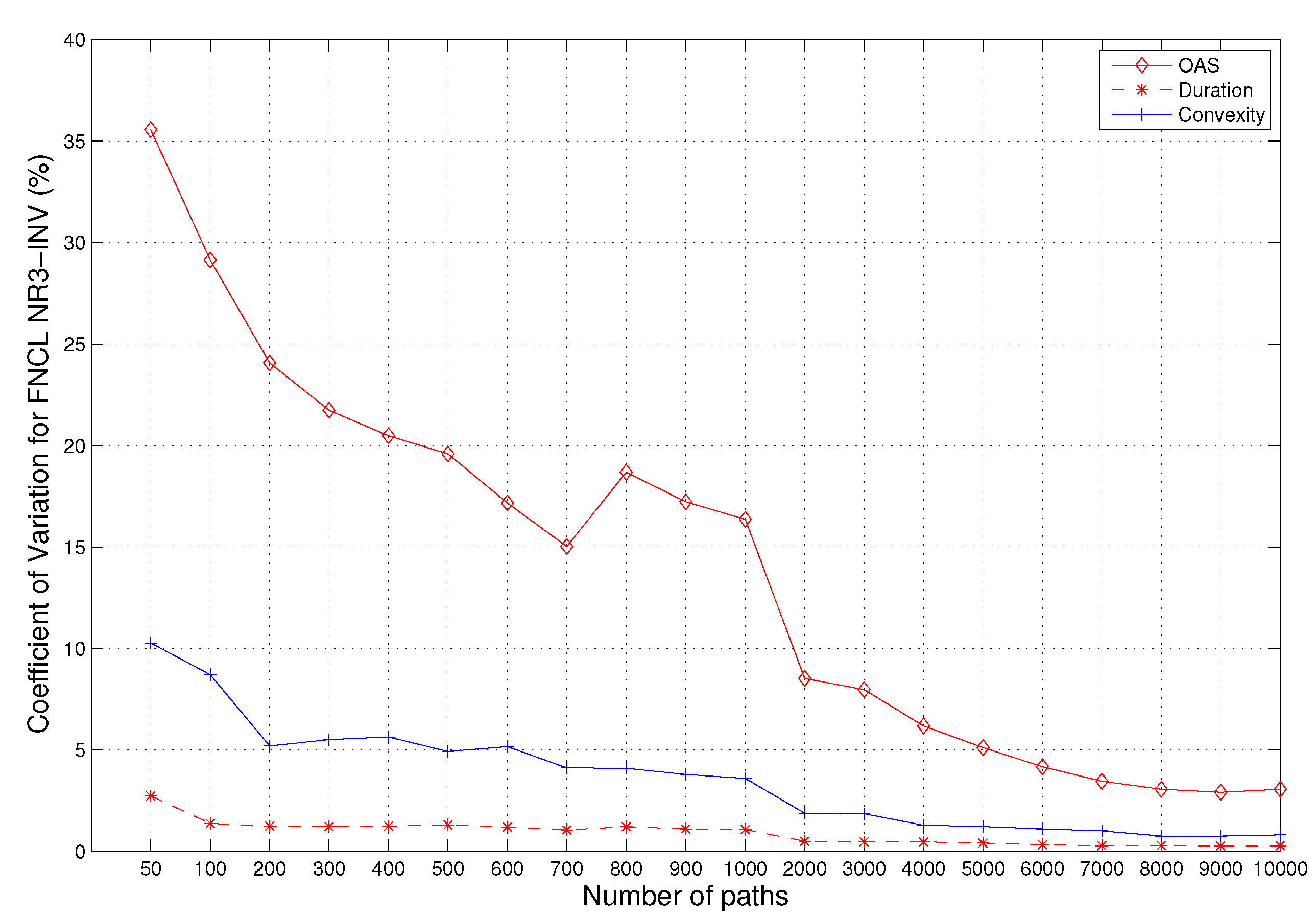
For any given random number generator combination and any of the three MBS instruments we consider, although OAS, DUR and CNVX all show convergence behavior as the number of paths increases, their convergence speeds are different. To indicate this, we consider a particular combination, NR3-INV, for an MBS instrument, FNCL. The convergence behaviors for OAS, DUR and CNVX are shown in the Figure 3.
Figure 3. The Comparison of the convergence of OAS, DUR and effective convexity for the FNCL using NR3-inverse cumulative distribution function (INV). The vertical axis is for the coefficient of variation (%). The horizontal axis is the number of paths.
Ijfs 03 00136 g003
As we can see from the figure, although OAS does show convergence as the number of paths becomes bigger, the convergence speed is very slow, compared to the convergence of DUR and CNVX.
To quantitatively measure the speed of the convergence, we consider the relation between the CV and the number of paths that are needed to reach the required accuracy measured by the CV. The results are summarized in Table 1.
Table 1. Convergence results for FNCL using NR3-INV.
CV ( % ) 201052.510.50.1
OAS5002,0006,000 10 4 + 10 4 + 10 4 + 10 4 +
Duration50-50-50-1002,0002,000 10 4 +
Convexity50-1005002,0006,000 10 4 + 10 4 +
Degree of Absolute Convergence
(OAS, DUR/CNVX)5002,0006,000 10 4 + 10 4 + 10 4 + 10 4 +
Degree of Relative Convergence
(OAS, DUR/CNVX)50-1005002,0006,000 10 4 + 10 4 +
As we can see from Table 1, for the FNCL, the convergence speeds for its DUR and CNVX are much faster than its OAS. For example, from Table 1, we can see that, if we use the random generator NR3-INV, to reach an accuracy of 5 % for OAS, i.e., C V 5 % , the required number of paths are at least 6 , 000 . On the other hand, under the same conditions, to reach the accuracy of 5 % for DUR or CNVX, the number of paths is much less than that for OAS. From the table, we can see that, for FNCL, only 50 paths are needed to reach the accuracy of 5 % for DUR and only 500 paths are needed for the effective convexity.
In addition, from the table, we can see that, for a given number of paths, if the number is small, OAS may not demonstrate good convergence properties. Although OAS obtained at this moment is not so accurate, we can still use it to calculate DURs and CNVXs, which can show very good convergence properties even if we use the same number of paths to calculate them.
To obtain a good approximative value for OAS, we need to use many paths (at least 10 4 ). Then, we can use OAS to calculate DUR and CNVX. There is no doubt that with the ‘accurate’ OAS and relative large number ( 10 4 ) of paths, we can get ‘accurate’ values for durations and convexity. This is the absolute convergence, which can always be guaranteed by virtue of the law of large numbers. However, it takes a long time, which is not bearable in the industry.
However, from our numerical results for FNCL, we can see that even if the numbers of paths are small and OAS does not show a very decent convergence property, DUR and CNVX can show a very nice convergence behavior. This is the relative convergence.
In Table 1, we also give the degrees of absolute convergence for OAS and DUR/CNVX, which are the number of paths that are needed for both OAS and DUR/CNVX to reach certain accuracy (CV) levels. The degrees of relative convergence, the numbers of paths that are needed for DUR/CNVX to reach certain accuracy (CV) levels, are given in Table 1, too. As we can see, the degree of absolute convergence is always larger than the degree of relative convergence, unless both of them are beyond 10 4 . For the latter case, although we do not have accurate values for the degrees of absolute convergence and relative convergence, we can tell from Figure 3 that the degree of absolute convergence is always larger than the degree of relative convergence. Therefore, if our final goal is to get DUR/CNVX only, we can seek relative convergence instead of absolute convergence to save computational time.

4.4. Robustness

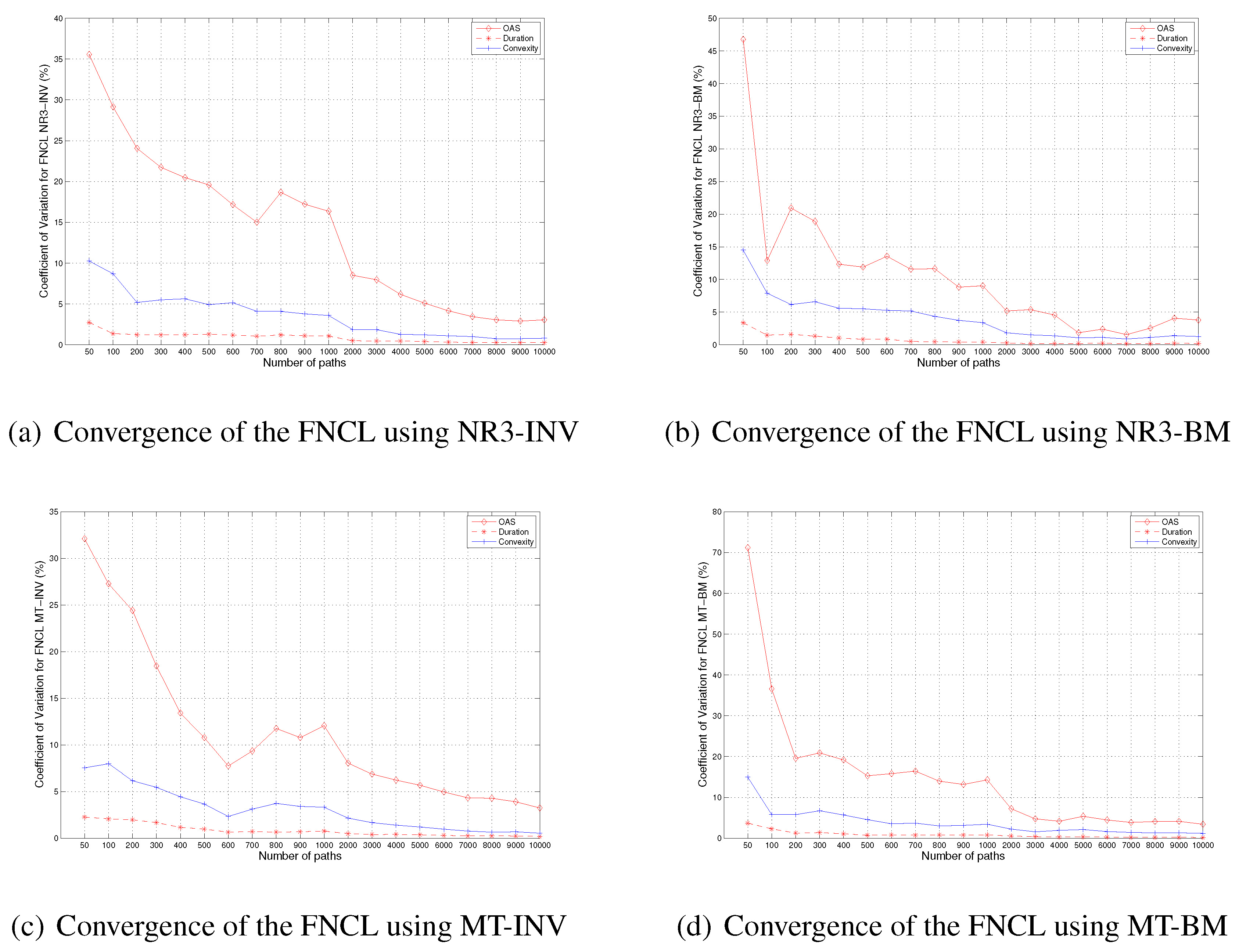
In the last subsection, we presented the numerical results for an MBS instrument, FNCL, using the random number generator combination RN3-INV. To test the robustness of the method, we also use another three random number generator combinations, NR3-BM, MT-INV and MT-BM, for our numerical experiments of FNCL. The numerical results are shown in Figure 4 (we put the results for NR3-INV here also for comparison purposes).
Figure 4. The Convergence of OAS, DUR and CNVX of the FNCL using different random number generator combinations, NR3-INV, NR3-Box–Müller (BM), Mersenne twister (MT)-INV and MT-BM. The vertical axis is for the coefficient of variation (%). The horizontal axis is the number of paths.
Ijfs 03 00136 g004
As we can see from the figure, for NR3-BM, MT-INV and MT-BM, the convergence patterns of OAS, DUR and CNVX are very similar to the pattern when we use NR3-INV.
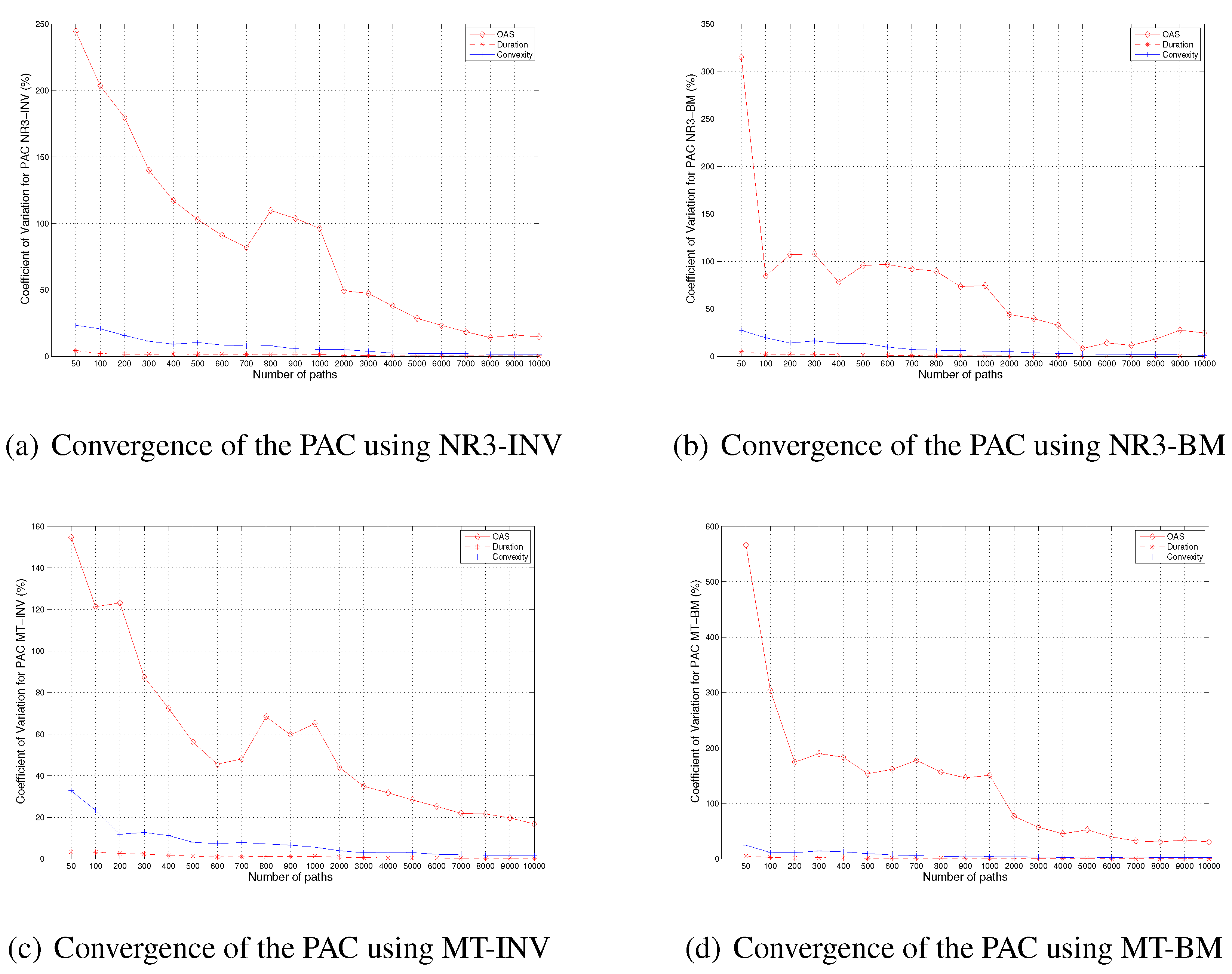
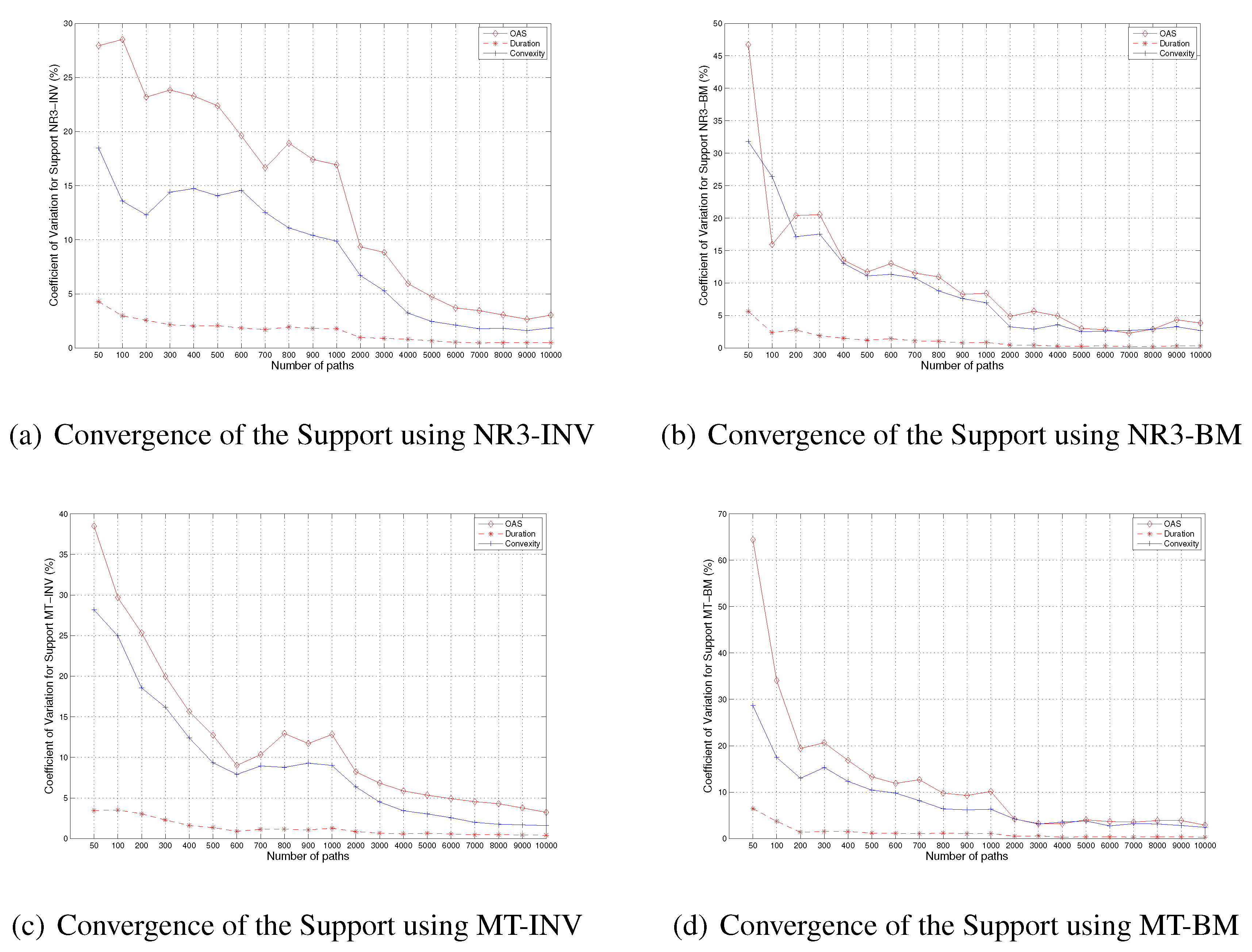
In addition, we repeat the numerical experiment for the other two MBS instruments, the PAC and the Support. The numerical results are given in Figure 5 and Figure 6.
As we can see from all of those figures, for all scenarios that we considered, we do observe the phenomenon that DUR and CNVX converge faster than OAS. Therefore, it is safe to say that relative convergence does exist for MBS securities when we use the typical pseudo-random number generators for our Monte Carlo Simulation.
Figure 5. The Convergence of OAS, DUR and CNVX of the planned amortization class (PAC) using different random number generator combinations, NR3-INV, NR3-BM, MT-INV and MT-BM. The vertical axis is for the coefficient of variation (%). The horizontal axis is the number of paths.
Ijfs 03 00136 g005
We want to point out that the relative convergence patterns for the FNCL, the PAC and the Support are somewhat different from each other. Although the DURs for all three MBS instruments have strong relative convergence patterns, the situation for CNVX is very different. From the figures, we can see that the convergence of CNVX is very fast for PAC. For the FNCL, the convergence of CNVX is slower than that of the PAC, but faster than that of the Support. This is not very surprising since PAC is the senior tranche and its duration is less sensitive to the prepayment and interest rate change, compared to the pass-through and the Support. On the other hand, the Support absorbs most of the prepayment, and its price and duration are more sensitive to the interest rate movement.
In addition, we observe that the relative convergence of DUR is stronger than that of CNVX for all three MBS instruments that we considered. In other words, to obtain the desired accuracy in terms of CV, the number of paths needed for DUR is less than that needed for CNVX, while the number of paths needed for OAS is the largest. Therefore, the convergence speed for DUR is the fastest, followed by that for CNVX and OAS. This is true for all three MBS instruments that we considered.
From our numerical results, we can see that if our final goal is to calculate the effective duration and CNVX for an MBS instrument, it is not necessary to use tens of thousands of paths to obtain an ‘accurate’ OAS first. Instead, in most cases, several thousands or several hundreds of paths are enough to get very accurate values of DUR and CNVX.
Figure 6. The Convergence of OAS, DUR and CNVX of the Support using different random number generator combinations, NR3-INV, NR3-BM, MT-INV and MT-BM. The vertical axis is for the coefficient of variation (%). The horizontal axis is the number of paths.
Ijfs 03 00136 g006

5. Conclusions

In this paper, we study the convergence behaviors of OAS, DUR and CNVX for three MBS instruments using Monte Carlo simulation. Instead of seeking very good accuracy for OAS before calculating DUR and CNVX, we propose a method to seek the the accuracy of DUR and CNVX directly.
We perform numerical studies for three different types of MBS instruments (pass-through, PAC, Support) and four random number generator combinations. The numerical results indicate that there does exist a phenomenon of relative convergence for all of the scenarios that we consider. In other words, although we need to use OAS to obtain DUR and CNVX, DUR and CNVX can reach a desired accuracy (measured in terms of CV) even though OAS has not reached very good accuracy. Therefore, if we just want to obtain good estimation of DUR or CNVX, it is not necessary to obtain good estimation for OAS first.
Given our results, now practitioners in the industry can save tremendous time and computational time when they evaluate the DUR and the CNVX of MBS instruments. For example, from Table 1, to reach an accuracy of 2 . 5 % for the DUR of the FNCL bond, instead of using 10 4 paths to obtain a good value of OAS, we can just use 100 paths to calculate OAS and then use OAS and 100 paths to obtain DUR, which has our desired accuracy. Put differently, it can save computation time by 99% in this particular example.

Author Contributions

All three authors contributed to the writing of this paper. In addition, the first author and the third author initiated this research project. The first author also provided the mathematical modeling for the project. The second author contributed to the simulations and data collection. The third author also provided the software platform for doing the simulations.

Conflicts of Interest

The authors declare no conflict of interest.

References

  1. P. Glasserman. Monte Carlo Methods in Financial Engineering. New York, NY, USA: Springer, 2003. [Google Scholar]
  2. F.J. Fabozzi. Fixed Income Mathematics, 4th ed. New York, NY, USA: McGraw-Hill, 2006. [Google Scholar]
  3. R.E. Caflisch, W. Morokoff, and A. Owen. “Valuation of Mortgage Backed Securities Using Brownian Bridge to Reduce Effective Dimension.” J. Comput. Financ. 1 (1997): 27–46. [Google Scholar]
  4. S.F. Richard, and R. Roll. “Prepayments on Fixed-Rate Mortgage Backed Securities.” J. Portf. Manag. 15 (1989): 73–82. [Google Scholar] [CrossRef]
  5. F. Black, and P. Karasinski. “Bond and Option Pricing when Short Rates are Lognormal.” Financ. Anal. J. 47 (1991): 52–59. [Google Scholar] [CrossRef]
  6. W. Press, S. Teukolsky, W. Vetterling, and B. Flannery. Numerical Recipes in C, 2nd ed. Cambridge, UK: Cambridge University Press, 1992. [Google Scholar]
  7. S.K. Park, and K.W. Miller. “Random number generators: Good ones are hard to find.” Commun. ACM 31 (1988): 1192–1201. [Google Scholar] [CrossRef]
  8. D. Kahaner, C. Moler, and S. Nash. Numerical Methods and Software. Englewood Cliffs, NJ, USA: Prentice Hall, 1989. [Google Scholar]
  9. D.E. Knuth. The Art of Computer Programming, Volume 2: Seminumerical Algorithms, 2nd ed. Boston, MA, USA: Addison-Wesley, 1981, Chapter 3.2–3.3. [Google Scholar]
  10. M. Matsumoto, and T. Nishimura. “Mersenne twister: A 623-dimensionally equidistributed uniform pseudorandom number generator.” ACM Trans. Model. Comput. Simul. 8 (1998): 3–30. [Google Scholar] [CrossRef]

