Abstract
In this paper, based on Generalized Autoregressive Conditional Heteroskedasticity (GARCH) model, five financial serials are dynamically weighted, and then China’s Financial Conditions Index is synthesized to measure China’s financial cycle. After that, using the monthly data of 2000–2023 as sample space, this paper utilizes the Markov Switching (MS) model to analyze the characteristics of China’s financial cycle and to investigate the four-zone system. Then, the Vector Autoregression (VAR) model focuses on investigating the macroeconomic effects of China’s financial cycle. The findings are as follows: Firstly, the dynamic weighting approach based on GARCH model is more suitable for valuating China’s financial cycle. Secondly, China’s financial cycle has a strong inertia at the state of transition and the imbalance of China’s overall financial situation is very common. Additionally, China’s financial cycle is distinctly characterized by the double asymmetry of fewer contractions and more expansions, shorter expansions, and longer expansions. Thirdly, China’s financial expansion offers a nine-month short-term stimulus to output and exerts lasting upward pressure on prices.
1. Introduction
The role of finance in the economy is complex, acting as both a catalyst for growth and a potential source of risk. A well-functioning financial system can significantly enhance the allocation of resources, fostering economic development. However, the financial system also harbors inherent instability that can lead to crises and economic imbalances. Despite its importance, the destabilizing effects of financial factors were largely overlooked in mainstream economic research until the global financial crisis of 2008. The crisis brought to light the deep interconnections between financial stability and broader economic health. Following this, scholars like Y. Chen and Ma (2013) and C. Borio (2014) have worked to incorporate financial stability into macroeconomic theory, recognizing its crucial role in ensuring long-term economic equilibrium.
China’s financial system has undergone a complex transformation since the country’s reform and opening up. The overall financial operation in China can be characterized by a dynamic balance between periods of relative stability and phases of heightened risk. However, the inherent volatility of China’s financial system poses significant systemic risks, which presents a formidable challenge for the government’s ability to regulate and stabilize the economy. In this context, understanding the underlying trends of China’s financial fluctuations, as well as their broader economic implications, becomes critical. A comprehensive assessment of these financial conditions is essential for formulating effective macroeconomic policies that not only safeguard financial stability but also ensure sustainable economic growth in the long run.
On the basis of existing studies, this paper focuses on accurately measuring China’s financial cycle. Then, it pays more attention to the analysis of the characteristics and macroeconomic effects of China’s financial cycle. Compared with the earlier literature, the main contribution of this paper is as follows. Firstly, GARCH model for dynamic empowerment is used to synthesize China’s FCI for the first time, which is a new exploration for the measurement of China’s financial cycle. Secondly, MS model, often used in the field of economic cycle but still less used in the field of financial cycle, is used to analyze the nonlinear dynamic characteristics of China’s financial cycle. Additionally, this paper deals with the issue of four-zone systems, such as the boom, recession, depression and recovery system, which can offer a beneficial supplement to the existing research.
In the following sections, this paper will first present the literature review on financial cycle measurement and characteristics, providing a theoretical foundation for the subsequent analysis. Section 3 details the methodology employed in this study, highlighting the dynamic weighting approach used for constructing China’s Financial Cycle Index (FCI). Section 4 investigates the distinctive characteristics of China’s financial cycle, utilizing a Markov Switching (MS) model to analyze its phase transitions. Section 5 explores the macroeconomic effects of the financial cycle, specifically examining its impact on output and price fluctuations through a Vector Autoregressive (VAR) model. Finally, Section 6 concludes the paper by summarizing the key findings and offering policy recommendations aimed at enhancing the stability and sustainability of China’s financial system.
2. Literature Review
The theory of financial cycle can be traced back to the 19th century. According to Niemira and Klein (1994), Mill divided the credit cycle into several stages early in 1867. Then, Wicksell took advantage of his natural rate hypothesis to explain the expansion and contraction of capital accumulation, which vigorously encouraged scholars to focus on the financial factors of economic fluctuation. Based on the related theories of Keynes and Fisher, Minsky (1977) put forward the theory of financial instability, which is aimed at directly studying financial cycles. At the late end of last century, Niemira and Klein (1994) first proposed the concept of financial cycle, observed monetary cycle, credit cycle, and interest rate cycle. Since 2008, the number of related empirical studies rapidly grew, but overall studies are still very limited, mainly focused on two aspects: measuring financial cycles and exploring the characteristics of financial cycles.
The measurement of financial cycles generally follows two paths. Firstly, many scholars use the concept of economic cycle defined by Burns and Mitchell (1946) to define financial cycles, taking financial cycles to mean periodic fluctuations among a large number of financial series rather than among a handful of financial series. Goodhart and Hofmann (2001) selected interest rate, exchange rate, house price, and stock price to meet the synthesis of the FCI among G7 countries. Schüler et al. (2015), from the Central Bank of Europe, selected credit, house price, stock price, and yield rate on bonds to extract common components. Ma and Zhang (2016) selected seven indicators, including real effective exchange rate, the growth rate of M2, house price, stock price, bank interest margin, long-term interest rate, and risk premium to synthesize the financial cycle index among the US, UK, China and Japan. Balfoussia et al. (2018), from the European Central Bank system, valuated the volatility of seven financial series in several countries in the Euro-zone, emphasizing the importance of ‘a high number of series moving together at business-cycle frequencies’ in the evaluation of financial cycles. C. E. Borio et al. (2019) argue that financial cycles, which capture periodic fluctuations across multiple financial variables, like credit, property prices, and leverage, serve as better predictors of recession risks compared to the term spread, especially for advanced and emerging economies. Xiong and Zhang (2018) elected 14 indicators to synthesize China’s FCI. Wang (2005), J. Lu and Liang (2007), Feng et al. (2012), Deng and Xu (2014), Liu and Li (2018) used four to seven quantitative indicators to synthesize China’s FCI, respectively. Miao et al. (2018) directly described China’s financial cycle by the respective fluctuations of multiple financial series. X. Lu et al. (2024) constructed China’s financial cycle index using key indicators like credit, credit-to-GDP ratio, housing prices, and stock prices, finding that financial cycles reflect periodic fluctuations across multiple financial variables, with dynamic interactions between financial and economic cycles. Secondly, according to C. Borio (2014), some scholars define financial cycles by seeking for the smallest set of variables to reflect financial fluctuations. C. Borio (2014), an expert from the Bank of International Settlement, argues that financial cycles areself-reinforcing interactions between perceptions of value and risk and attitudes towards risk and financing constraints. In addition, credit and property prices are the smallest set of variables needed to adequately replicate the mutually reinforcing interaction between financing constraints and perceptions of value and risk. Drehmann et al. (2012), another expert from BIS, Praet (2016), European Central Bank Executive Boarder, and Claessens et al. (2012), from IMF, favor this kind of definition and measurement. Meanwhile, many Chinese scholars such as Yi and Zhang (2016), Fan et al. (2017), and Zhu and Huang (2018), adopted this definition and made use of it to measure China’s financial cycle.
During the process of measuring financial cycles, the selection of representative variables is very crucial. The above-mentioned definition and measurement from Borio takes into account all financial activities, such as the interaction between credit and property prices. Its essence is to define the financial cycle from the portfolio behavior of economic entities. This approach has a good micro-foundation and the strength of convenient calculation, but it cannot avoid the risk of missing important information. Additionally, the heterogeneity among financial markets in different countries makes it difficult to apply the variables selected from a certain country to other countries. In fact, financial activity is extremely extensive and, using fluctuations among a large number of financial variables to characterize financial cycles, can effectively avoid the risk of missing important information. Meanwhile, the above-mentioned literature also demonstrates that many scholars have neglected the connection between financial cycle and monetary policy during the process of the selection of financial variables. The purpose of constructing FCI is not only to serve financial and economic forecasting but also to find a suitable substitute for the existing intermediate objectives of central banks’ monetary policy. Therefore, FCI’s compositional variables should have the dual attributes of the intermediate objectives for monetary policy: (1) Relevance: they are able to affect prices and output. (2) Controllability: they are at the control of the central bank. For this reason, synthesizing FCI with more variables is not preferred.
In addition to the selection of financial variables, variable weighting is also a key step to measure financial cycle. Up until now, the literature has mainly adopted the following methods: (1) Large-scale macroeconomic model. Dudley and Hatzius (2000) made use of the Fed’s macroeconomic model to construct America’s FCI by estimating the impact of variables on GDP and realized the variables’ weighting. (2) Simplified aggregate demand model. Goodhart and Hofmann (2001) incorporated asset prices into the standard aggregate demand simplified equation to allocate weights by estimating the impact of financial variable gaps on output gap. After that, Swiston (2008) synthesized America’s FCI. J. Lu and Liang (2007) synthesized China’s FCI. (3) Impulse response functions in VAR model. Goodhart and Hofmann (2001), Gauthier et al. (2004), respectively, constructed VAR models and used impulse response to analyze and to determine variable weights. Feng et al. (2012) used VAR model to test and synthesize China’s FCI. Nakajima et al. (2011) developed TVP-VAR model, which offers tools for the dynamic weighting of FCI’s compositional variables. Then, Koop and Korobilis (2014) constructed UK’s FCI, and Deng et al. (2016) and Liu and Li (2018) set up China’s FCI. Jabeenm and Qureshi (2019) constructed Pakistan’s FCI using a time-varying method involving models like TVP-FAVAR and FA-TVP-VAR. (4) Principal component analysis. Principal component analysis turns the original component variables of FCI into a group of unrelated comprehensive indicators. Then, the contribution rate of each principal component is taken as the corresponding weight to synthesize FCI. For example, Vonen (2011) developed a monthly FCI for Norway by employing principal component analysis on 13 financial variables and demonstrated its effectiveness as a leading indicator of GDP growth. Angelopoulou et al. (2014) constructed FCIs for the Eurozone from 2003 to 2011, incorporating various financial variables and studying the impact of monetary policy on financial conditions. Deng and Xu (2014), Xiong and Zhang (2018) respectively synthesized China’s FCI.
The above-mentioned empowerment approaches have both advantages and disadvantages. The weighting results of the large-scale macroeconomic model are often convincing if the model itself can accurately simulate the economic reality. But, the current macro models various central banks use have not included the key element-asset prices. Additionally, it involves a large amount of data collection and complex data processing work, which greatly limits the scope of its application. The set including the simplified aggregate demand model is firmly based on the theory of monetary policy transmission mechanism, but the endogenous issue of variables brings many obstacles to identification and parameter valuation. Impulse response functions in VAR model are not subject to specific economic theory and their parameter valuations are easy to realize by impulse response analysis, but it cannot acquire any structural explanation in terms of parameter valuation. Principal component analysis can realize the observation in a wide range of financial variables by dimension reduction processing, and it is not subject to specific theory. However, the economic meaning of principal components is difficult to explain and the contribution of each primitive variable in FCI is difficult to decompose. At the same time, aside from the empowerment approach of TVP-VAR model, the other approaches all belong to methods of fixed weighting, which cannot match with reality. In essence, a country’s economic structure, financial system, and even the efficiency of each transmission channel of monetary policies are in a dynamic process. In different periods, the financial variables in the overall financial situation of a country tend to change in terms of the relative importance. Therefore, the variable weighting in measuring the financial cycle should be a kind of dynamic approach and the results obtained by the fixed weighting method may greatly deviate from the reality.
As for the exploration of the characteristics among financial cycles in the existing literature, an important method is to observe the international co-movement. For example, Balfoussia et al. (2018), X. Chen and Zhang (2017), and Han (2018) observed the consistency among financial cycles in different countries and regions. Sun et al. (2020) also found significant co-movement among financial cycles in different countries and regions, especially in terms of cross-border capital flows. Another important branch is the identification of different components with different frequencies in financial fluctuations and the relative importance of different components. C. Borio (2014) used BP filters to extract short-term components and medium-term components in terms of the credit and social financing scale, emphasizing that the medium-term component is more important than the short-term component. Using univariate filters, Drehmann et al. (2012) and Aikman et al. (2014) found evidence of mid-cycle among credit and house prices. Using turning point analysis, Claessens et al. (2012) drew similar conclusion. Balfoussia et al. (2018) used band-pass filter and wavelet analysis to investigate the basic attributes of seven financial series’ cyclical components in several countries in the euro-zone. They also used the multivariate structural time series model (STSM) to examine house price cycle, credit cycle, and GDP cycle. Their study found that there were no medium cycles of house price fluctuation and credit fluctuation in some countries. Meanwhile, the characteristics of house price fluctuation and credit fluctuation in different countries may be related to the inherent structural characteristics of the housing market. Using BP filter, Yi and Zhang (2016) extracted and compared the medium-term component and short-term component of China’s financial fluctuation. They pointed out that there was no evidence that the former is more important than the latter. Fan et al. (2017) directly extracted and observed the medium-term component of China’s financial fluctuation. Zhu and Huang (2018) pointed out that there were obvious deviations in the bandwidth setting of BP filter in previous research. They clearly demonstrated that China’s financial fluctuation was different from the financial fluctuations in developed countries. They concluded that the short-term component was more important than the medium-term component in terms of China’s financial fluctuation. Using the bandpass filter approach, Ali Hardana et al. (2023) found that an increase in credit growth over the past century has always been accompanied by an increase in the probability of a banking crisis. Similarly, studies such as Tian et al. (2024) have used BP filters to extract medium-term financial cycles, particularly in credit and housing prices, and found that these cycles were more stable and had longer durations compared to asset price cycles. The study highlighted the synchronization of medium-term cycles across countries, especially during global financial crises, confirming the interconnectedness of financial systems globally. In addition, few scholars utilized the MS model to observe the characteristics of China’s financial cycle. For example, Deng and Xu (2014) observed the expansion and contraction of the two-zone system and the three-zone system, that is, the low, medium and high area. However, it cannot reflect the four-zone system, that is, boom, decline, depression and recovery, which is often a topic in economic cycle study. Yao et al. (2021) extracted financial cycles based on the financial conditions index and BP filter, and used the MS model to analyze the nonlinear effects of financial cycles on systemic financial risks across different financial industries under various market states.
According to the literature summary above, it can be concluded that the measurement of financial cycles has undergone significant development, particularly in the context of emerging markets. Fixed-weight composite indices have long been a cornerstone for capturing cyclical co-movements, but their static nature fails to account for volatility clustering and time-varying risk spillovers, especially in the context of China’s financial system. Recent approaches, such as regime-switching models, have improved phase identification but rely on subjective thresholds and fail to capture policy-driven inertia. Additionally, while studies on macroeconomic spillovers emphasize the nonlinear effects of financial shocks, few address the temporal asymmetry between short-term output boosts and long-term inflationary pressures, a critical gap given China’s cyclical stimulus policies. The lack of focus on these dynamics motivates the following hypotheses:
Hypothesis 1.
The dynamic weighting method, based on the GARCH model, provides a more accurate representation of China’s financial cycle compared to fixed-weight models.
Hypothesis 2.
China’s financial cycle exhibits a four-phase structure (boom, decline, depression, and recovery), reflecting significant inertia in financial conditions, which differs from the more frequently studied two-phase or three-phase systems.
Hypothesis 3.
The financial cycle significantly influences macroeconomic indicators such as output and price fluctuations.
These hypotheses aim to address the gaps in the existing literature by introducing dynamic weighting and a four-phase financial cycle framework to more accurately measure the volatility of China’s financial cycle and explore its macroeconomic effects. By testing these hypotheses, this study seeks to provide new insights and evidence for both the theory of financial cycles and the policy implications for China’s economic regulation.
Moving forward, as a kind of exploration and necessary supplement to the existing research, this paper selects appropriate variables to reflect China’s overall financial situation based on the analysis of monetary policy transmission channels. Additionally, it uses the GARCH model to dynamically weigh the variable gap values for the first time. Then, it brings the synthesis of China’s FCI, which can realize the calculation of China’s financial cycle. After that, this paper uses the MS model to analyze the nonlinear dynamic characteristics of China’s financial cycle and, for the first time, to observe the boom, decline, depression, and recovery in China’s financial cycle. Finally, this paper uses the VAR model to examine the macroeconomic effects of China’s financial cycle. All these works can offer credible and empirical evidence for real-time monitoring on China’s overall financial situation and policy selections for China’s macroeconomic regulation.
3. Measurement of China’s Financial Cycle, Based on Dynamic Weighing Approach
3.1. Synthesis of China’s FCI on Variable Selection
Different financial variables have impacts on economic running through specific channels. The central bank uses monetary policy instruments to influence these financial variables. Accordingly, there are many channels for monetary policy transmission as follows. The first one is credit. The central bank uses required reserve ratio, re-loans, and other tools to regulate the scale of credit, which affects enterprise investment and household consumption, then ultimately makes a difference to prices and output. The second one is interest rate. The central bank uses open-market operation and rediscount policy to guide the changes of short-term interest rate in financial markets, which can then affect the return on investment. After that, it can affect investment, which ultimately affects output and prices. The third one is exchange rate. It contains two branches, such as foreign trade and capital flow. In terms of foreign trade, exchange rate fluctuations under the regulation of central bank can lead to export fluctuations, which can change aggregate demand, which ultimately affects output and prices. In terms of capital flow, exchange rate fluctuations under the regulation of central bank affect the inflow and outflow of foreign capital, which can change the domestic money supply. After that, it affects aggregate demand and ultimately changes prices and output. The fourth one is asset prices. The asset prices affect economic running through the “wealth effect” and “balance sheet effect”. The fluctuations of asset prices mean that household wealth levels fluctuate, which affects consumer demand. After that, it ultimately affects output and prices. The fluctuation of asset prices also means that the changes in household assets and liabilities, and the changes in financing constraints, affect consumption, investment, and ultimately, output and prices. The above-mentioned four channels play an important role in China’s monetary policy. Meanwhile, it should be noted that money supply has always served as an intermediate target for China’s monetary policy during the process of economy regulating since 2000, and it has an extremely important position in China’s financial system. The change in money supply not only reflects the direction of monetary policy but also directly reflects the changes in the overall liquidity of financial markets. Therefore, in the process of constructing China’s FCI, we cannot ignore its influence.
Based on the above-mentioned analysis, taking credit and monetary supply with a high degree of overlap into consideration, this paper finally chooses five variables as variable sets, such as monetary supply, social financing scale, stock price, interest rate and exchange rate. After the synthesis of the FCI, it can reflect the financial cycle of China.
3.2. Explanation of Data Source and Processing Method
According to the criteria of rationality and availability, this paper takes the monthly data of various series from 2000 to 2023 as the sample space. There are 288 observation points in total. This paper contains seven indicators all together: (1) Five indicators, such as monetary supply, social financing scale, stock price, interest rate, and exchange rate are used to synthesize China’s FCI. (2) Two indicators, such as the rate of output growth and the rate of the inflation, are used to reflect China’s macroeconomic conditions. As for the seven indicators, we take, in turn, M2, Social Financing Scale Index, Shanghai Composite Index (closing price), the weighted average interest rate of inter-bank lending (7 days), real effective exchange rate index, the growth rate of the added value of financial sector, and the consumer price index (CPI) as proxy indicators. Because real quantity rather than nominal quantity makes a difference to the behavior of economic subjects, it is necessary to turn the nominal quantities into real ones. Among the seven indicators, it is not necessary to remove the impact of inflation in terms of the CPI. Meanwhile, the social financing scale index, the real effective exchange rate index, and the growth rate of the added value of financial sector are already real quantities. Therefore, it is necessary for the other three indicators to experience de-inflation processing: (1) Real interest rates are obtained by deducting year-on-year CPI inflation from nominal interest rates. (2) Taking 2000 as the base period, M2 and stock price CPI are deflated by fixed base price index, respectively. Then, we can obtain the actual M2 and stock price. Moving forward, the actual quantities of the seven indicators have experienced seasonal adjustment by X12. There is some information in Table 1.

Table 1.
Symbol of the indicators, data source, and processing method.
3.3. The Synthesis and the Results of China’s FCI
3.3.1. Dynamic Weighting of Compositional Variables in China’s FCI
1. To obtain the gap value of each variable and to make them dimensionless, time series consists of multiple components and the measurement of financial cycle focuses on the cyclical component. Therefore, according to the suggestion from Drehmann and Yetman (2018), the seven series from Table 1 experienced the process of the HP filter (matching with monthly data filtering, the value of the parameter is 14,400). Then, we can obtain the absolute gap—the periodic component and the equilibrium value-trend component. Moving forward, before the synthesis of the FCI, it is necessary to root out the difference of dimension among variables. Therefore, as for the four variables, M2, social financing scale index, stock price index and real effective exchange rate index, the absolute gap is divided by the corresponding equilibrium value, respectively, to obtain the relative gap (similar to growth-rate or yield rate). It can be shown in the formula as follows.
Among them, represents the actual value and means the equilibrium value in terms of the variable at the time stage of . Where is the absolute gap, is the relative gap. For the short-term interest rate, the absolute gap is considered as the gap value, because it is already relative in percentage. The expression is as follows.
The gap values of all variables are obtained after the mentioned processing, which is unified as a dimensionless percentage. ADF test shows that they are all stable series and meet the premise of stable sequence required for time series analysis. The results can be reflected in Table 2 in detail. In order to be more convenient, GAP_M2, GAP_SFC, GAP_SP, GAP_REER and DEL_IR represent the gap value of five variables, such as M2, SFC, SP, REER and IR.
Table 2.
Unit Root Test of ADF among the Five Gap Value from Financial Sequence.
2. Dynamic Weighting based on Approach of GARCH model. The GARCH model, which was originally proposed by Bollerslev (1986), is widely used for analyzing financial time series with heteroskedasticity. Since financial variables such as stock prices, exchange rates, and interest rates often exhibit time-varying volatility, GARCH models provide a better estimation of dynamic risk structures compared to constant variance models. In particular, this paper employs the GARCH(1,1) specification, as it is the most commonly used and parsimonious form of GARCH models, capturing both short-term persistence and long-run volatility clustering effectively. Compared with higher-order models like GARCH(2,1) or GARCH(1,2), the GARCH(1,1) model provides a balance between flexibility and efficiency, avoiding potential overfitting while still accurately modeling the conditional variance of financial indicators. Also, it can measure the fluctuation of each sequence. This paper uses the GARCH (1,1) model to estimate the hetero-scedasticity. The expression is as follows.
Among them, is the current conditional variance, which can be taken as the weight of the residual squares of (), lagging for one period, and the variance of (), lagging for one period. This paper uses this model to estimate the gap values of the GAP_M2, GAP_SFC, GAP_SP, GAP_REER and DEL_IR. Then, it can reflect the conditional variance at different periods. On the basis of this, Ma and Zhang utilize the dynamic factor index model to construct the dynamic weighting. The dynamic weight is expressed as follows.
Among them, is the conditional variance for variable at the stage of . is the dynamic weight for variable at the stage of during the synthesis of FCI, which can be shown as , i = 1, 2, 3, 4, 5.
3.3.2. The Expression and the Synthesis of China’s FCI
1. The expression of China’s FCI. As for the quantities, China’s FCI is the weighted average of the gap values among five variables after seasonable adjustment. Economic theory and a lot of empirical research show that interest rate and real effective exchange rate (from BIS) are the reverse of overall financial conditions, while the others are consistent with them. Therefore, before the synthesis of China’s FCI, the two indicators, interest rate and exchange rate, are treated in reverse process (taking the opposites of their gap values), which can obtain the expression of China’s FCI.
There are four meanings behind Formula (7). Firstly, the combined fluctuation of the five indicators determines the fluctuation of China’s overall financial situation. Secondly, M2 fluctuation, social financing scale fluctuation, and stock price fluctuation all lead to the same direction of China’s overall financial situation. Thirdly, fluctuations in real interest rate and real effective exchange rate of RMB can lead to the reverse direction of China’s overall financial situation. Fourthly, the relative importance of the five indicators in China’s overall financial condition changes as time changes.
2. The results and the explanation of the synthesis of China’s FCI. This paper takes the gap values at different periods, such as GAP_M2, GAP_SFC, GAP_SP, DEL_IR and GAP_REER, and their dynamic weights into Formula (7). Then, there is the sequence of China’s FCI, shown in Figure 1.
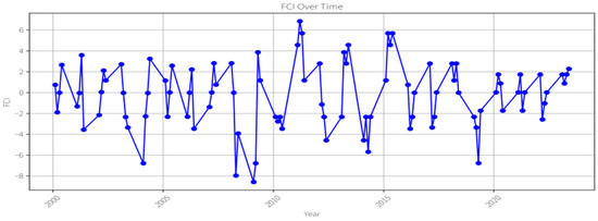
Figure 1.
The Trend of China’s FCI.
The synthesis of the FCI can reflect the gap values in terms of the variables expressed as a percentage. Therefore, the gap value of the FCI is expressed as a percentage. When the value of the FCI is equal to, greater than or less than zero, it can reflect the stages of equilibrium, loose and tense. Additionally, from the direction of the transmission, the expansion value of the FCI means the extension of the overall financial situation while the shrink value of the FCI means the shrink of the overall financial situation.
From the updated figures covering the period from 2000 to 2023, the FCI in China exhibits multiple fluctuations, characterized by rising, falling, and sustained cycles. The index ranges from approximately −8.57 (2009Q3) to 6.84 (2011Q2), indicating substantial volatility. (1) 2000Q1–2005Q4: period of high volatility. In early 2000, the FCI stood at 0.75 (2000Q1) but experienced a sharp decline to −1.89 (2000Q2), indicating a rapid tightening of financial conditions. By the fourth quarter of 2000, the FCI rebounded to 2.65, reflecting an expansionary phase, but this was followed by frequent fluctuations over the next few years. The lowest point in this phase occurred in the first quarter of 2004, with the FCI dropping to −6.8, showing a highly restrictive financial environment. This was likely due to tightening monetary policies and financial regulations during this period. (2) 2006Q1–2010Q4: expansion and the global financial crisis. From 2005 to 2009, the FCI showed a general upward trend. From 2006Q3, the FCI turned positive at 2.21, signaling improving financial conditions. By 2008Q1, the FCI peaked at 2.70, reflecting the financial expansion associated with booming stock markets and economic growth in China. However, after the 2008 global financial crisis, the FCI plummeted to its lowest point at −8.57 in 2009Q1. This sharp decline aligns with the crisis-induced liquidity crunch and global economic downturn. (3) 2011Q1–2015Q4: post-crisis adjustment and market cycles. After the post-crisis rebound, the FCI showed cyclical movement. It peaked at 6.84 in 2011Q2, reflecting the effects of financial stimulus and increased credit supply. However, the index then experienced a downturn, reaching −2.33 in Q4 2014, which coincided with regulatory tightening, deleveraging, and increasing concerns over financial stability. (4) 2016Q1–2023Q4: stabilization and recent trends. A significant drop occurred in 2019Q3 (−6.77), driven by factors such as slowing GDP growth (6.0%), U.S.–China trade tensions, tightened financial regulations, moderate monetary policies, stock and bond market volatility, real estate financing restrictions, and global economic uncertainty. However, since 2021Q1, the index has shown a steady recovery, reaching 2.28 in 2023Q4, reflecting policy adjustments aimed at stabilizing financial markets and supporting economic growth. These trends highlight the dynamic nature of China’s financial landscape, shaped by domestic policies and external economic forces. Overall, the updated FCI trends align with key economic and financial events in China, demonstrating the interaction between government policies, financial regulations, and global economic influences.
3. Comparison with the results of fixed weighting. Moving forward, based on the GARCH model, this paper estimates the dynamic weights of five gap values such as GAP_M2, GAP_SFC, GAP_SP, L_IR, and GAP_REER. According to the existing references, this paper uses the weighting method based on the simple arithmetic mean and the fixed weighting method based on homo-variance assumption, respectively. Then, there are the series of the FCI. Compared with the series of China’s FCI obtained by the dynamic weighting of GARCH model, the results can be reflected from Figure 2a,b. Among them, three weighs, that is, the dynamic weight obtained by the GARCH model, fixed weight obtained by simple arithmetic mean, and fixed weight obtained on the assumption of co-variance, are marked, respectively, as FCI1, FCI2, and FCI3.
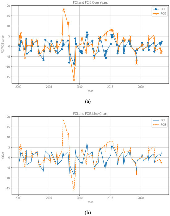
Figure 2.
The trend of China’s FCI. (a) The comparison between heteroscedasticity dynamic weight and simple average fixed weight. (b) The comparison between heteroscedasticity dynamic weight and co-variance fixed weight.
According to Figure 2a, in most periods, FCI2 and FCI1 (FCI) are not only similar in trend but also align in the timing of many peaks and troughs. However, in certain periods, such as 2008–2010, 2015–2016, and 2020–2021, it can be observed that FCI2 has the opposite sign and misinterprets the overall financial conditions. Furthermore, the maximum and minimum values of FCI2 are 18.4 and −16.5, respectively, while the maximum and minimum values of FCI1 (FCI) are 6.84 and −8.57, indicating that FCI2 overestimates the actual fluctuations. According to Figure 2b, the trend of FCI3 is similar to that of FCI1 (FCI), suggesting that the results of FCI1 (FCI) are relatively stable. However, during 2009–2010 and 2016–2017, FCI3 exhibits an opposite sign, misinterpreting the overall financial conditions. Additionally, the maximum and minimum values of FCI3 are 17.9 and −17.1, respectively, showing that, while it provides a reasonable estimation of financial fluctuations, certain deviations still exist in specific periods. Therefore, compared with other methods, the dynamic weighting approach based on the GARCH model used in this paper to synthesize China’s FCI better aligns with the reality of financial conditions in China.
4. The Analysis of the Characteristics in China’s Financial Cycle, Based on MS Model
4.1. The Applicability and Settings of MS Model
Since 2000, China’s financial cycle Composite Index (FCI) has experienced many significant ups and downs, and these changes are not only frequent but also drastic, which fully demonstrates the characteristics of phase transition in financial cycle. Faced with such data characteristics, we recognized the need for an analytical tool that could capture such discreteness and nonlinearity. Therefore, this paper refers to the method of Wang et al. (2020) and adopts the MS model proposed by Hamilton (1989) to explore the characteristics of China’s financial cycle. A significant advantage of the model is its ability to effectively simulate discrete changes in time series data, which is particularly important for describing the dynamic characteristics of economic variables during phase transitions. In the financial market, the pace of the country’s financial opening, macro-control policies and market sentiment may fluctuate sharply in different periods, which reflects the complexity and variability of the financial cycle. The details of this model are as follows.
Among them, N is the number of the system (N = 2, 3 or 4). Where is state variable (i = 1, …, N), the variable is from state to state and the probability is . And the expected time in the state is 1/(1 − pii).
4.2. The Characteristics of China’s Financial Cycle
The regional division method of financial cycle is a complex and delicate process. One method is based on Markov regional transfer model, which divides the first-order difference series of financial situation index into two regions and obtains the start and end time of financial cycle in expansion state and contraction state, respectively. According to the connection between the start and end time of these two states (the intersection point of expansion and contraction is the peak, and the intersection point of contraction and expansion is the valley), the occurrence time of the inflection point of financial cycle can be determined so as to realize the investigation of the volatility characteristics of financial cycle. The other method is based on the combination of monetary cycle and credit cycle to form four different stages of “wide money + tight credit”, “wide money + wide credit”, “tight money + wide credit”, and “tight money + tight credit” to reflect the different regional systems of the financial cycle. In order to avoid the one-sidedness of a single method, this paper uses a two region system, three region system, and four region system for maximum likelihood estimation and obtains smooth probability graphs under the following three cases.
From Figure 3, The phase transition of China’s financial cycle is clearly described in the MS model under the two-zone system, three-zone system, and four-zone system, and these phase transition processes show high stability. Specifically, the self-sustaining probability of each system is high, which reflects the strong inertia of the phase transition of China’s financial cycle.
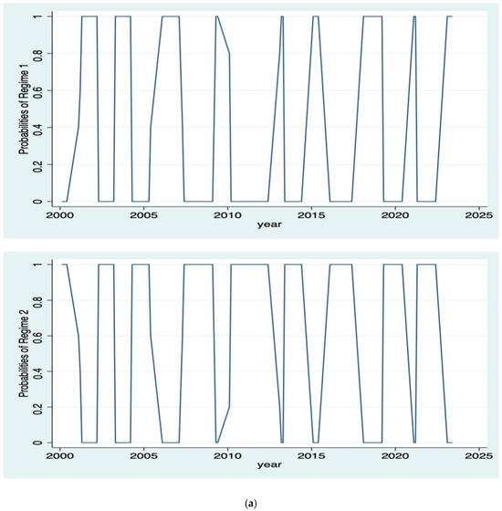
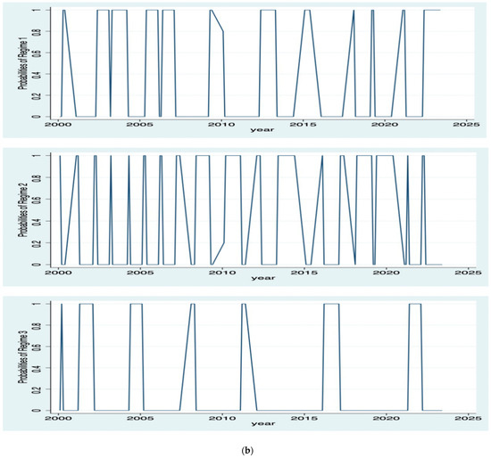
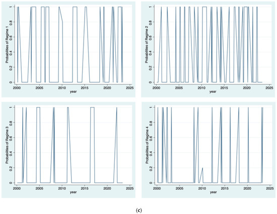
Figure 3.
(a) The probability results of the two-zone pattern in China’s FCI. (b) The probability results of the three-zone pattern in China’s FCI. (c) The probability results of the four-zone pattern in China’s FCI.
As shown in Table 3, in the two-zone system, the self-sustaining probabilities of economic contraction and expansion are 0.9179 and 0.9750, respectively. Based on these probabilities, we can calculate that the expected duration of the economic contraction is 12.18 months, and the expected duration of the economic expansion is 28.61 months.
Table 3.
China’s financial cycle in different systems.
Turning to the three-zone system, the self-sustaining probabilities of tension, moderation, and loose state are 0.9090, 0.8888, and 0.8965, respectively. Accordingly, the duration of the tension period is expected to be 10.99 months, the duration of the easing period is expected to be 8.99 months, and the duration of the easing period is expected to be 9.67 months.
In the four-zone system, the self-sustaining probabilities of recession, depression, recovery and prosperity are 0.8918, 0.7635, 0.7884, and 0.8931, respectively. Based on these probabilities, the recession is expected to last 9.24 months, the depression is expected to last 4.23 months, the recovery is expected to last 4.73 months, and the boom is expected to last 9.35 months.
To sum up, no matter what kind of system, each stage of China’s financial cycle shows a strong transition state inertia, which can be confirmed by the expected duration of each stage.
Moving forward, China’s financial cycle exhibits a distinct dual-asymmetry pattern under the Two-zone framework. Contraction phases occur with a probability of 31.59%, significantly lower than the 68.41% likelihood of expansion phases. This imbalance is further amplified by duration disparities, where expansion periods persist far longer than transient contractions. Such cyclical behavior underscores a structural bias toward growth, coupled with self-reinforcing inertia in state transitions, reflecting a financial ecosystem prone to prolonged expansions and abrupt, short-lived contractions. The three-zone diagnostic system reveals that imbalanced financial conditions prevail in 49.65% of observed periods, exceeding the frequency of stable moderation phases. This dominance of abnormal states—marked by either excessive tightness or looseness—highlights systemic vulnerabilities. The recurring imbalance suggests inherent instability in China’s financial operations, necessitating proactive monitoring to mitigate risks associated with prolonged deviations from equilibrium. Expanding to a four-zone framework, nearly half of all periods (48.25%) fall into extreme states (depression or boom), illustrating the system’s propensity for over-contraction or over-expansion. This polarization underscores the challenges of maintaining moderation, as extreme monetary conditions frequently dominate. Addressing this volatility requires countercyclical policies tailored to curb excessive fluctuations, particularly during extended booms, while ensuring targeted interventions to stabilize abrupt shifts between states.
In short, China’s financial cycle presents three outstanding characteristics: double asymmetry, normal imbalance, and extreme state polarization. First, the periodic operation follows the double asymmetric law of “low frequency short contraction” and “high frequency long expansion” (contraction probability 31.59% vs. expansion probability 68.41%), which reflects the characteristics of strong internal inertia and high policy dependence in the expansion stage. Second, the imbalance of the system became the norm, and 49.65% of the period deviated from the equilibrium state, reflecting the frequent overshoot of the financial environment between tightening and easing, and the weakness of the internal stability mechanism. Third, nearly half of the cycle stage (48.25%) fell into the “depression-overheating” extreme range, highlighting the structural contradictions of easy excessive policy transmission and difficult market expectation management. These characteristics together point to the operational nature of China’s financial cycle of “expansion leading, inertia strengthening, volatility polarization”, which requires the construction of differentiated macro-prudential tools, focusing on strengthening the risk mitigation mechanism between the expansion period and the transition calming mechanism between the extreme state.
5. The Macro-Economic Effects of China’s Financial Cycle
The fundamental goal of the synthesis of FCI is to serve as an important indicator for the government to offer the macro-economic policy, which can control financial risks and ensure smooth operation of the macro-economy. And, it demands that financial fluctuation precedes economic fluctuation and has a stable quantitative relationship with economic fluctuation. Therefore, this paper must take the macro-economic effects of China’s financial cycle into consideration. At the same time, the FCI is composed of multiple variables and not predictable, which means no systematically theoretic analyses of the core indicators among the output and price in terms of the fluctuation in financial cycle. For this reason, unconstrained VAR model is used for observation.
5.1. The Setting of Model and Stability Test
The month-on-month growth rate of the financial sector and the month-on-month growth rate of the CPI are considered as the proxies for the fluctuation of output and the fluctuation of price, which are expressed as R_FIN and R_CPI. This paper takes the mentioned FCI as the proxy of the fluctuation in China’s financial cycle and puts the two variables in VAR model, such as FCI1 and R_FIN, which can observe that the fluctuation of China’s financial cycle affects the fluctuation of the output and the fluctuation of the price. FCI1, R_FIN and R_CPI are stable series, and the unit root test is shown in Table 4.
Table 4.
The unit root test of ADF on output fluctuation and price fluctuation.
The meaning of C, T, and P is the same as in Table 2. The result of the R_CPI’s unit root test is a catastrophe point of the unit root test.
5.2. Granger Causality Among China’s Financial Cycle, Price Fluctuation and Output Fluctuation
Based on Model 1 and Model 2, this paper uses the Granger causality test to observe preceding relation and lag time in China’s financial cycle, price fluctuation and output fluctuation. The results are listed in Table 5.
Table 5.
Results of Granger causality test in China’s financial cycle, price fluctuation and output fluctuation.
Using the rule of the information among AIC, HQ and FPE, the above-mentioned two models can be determined as the fifth period and the fourth period in terms of the lagging term. From the Figure 4, the two models are very stable and can experience the analysis of the effective impulse response, which can be shown in Figure 4a,b.
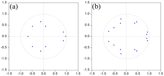
Figure 4.
AR Root Test. (a) Test in Model 1. (b) Test in Model 2.
From Table 5, (1) in Model 1, the null hypothesis that the change in FCI1 does not granger causes the change in R_FIN is rejected at 1% significant level and the original hypothesis that the change in R_FIN does not granger causes the change in FCI1 is rejected at 10% significant level. This reflects how there is a bilateral granger causality between the financial fluctuation and output fluctuation. China’s financial fluctuation is a leading indicator of output fluctuation, which can serve as an early warning of output fluctuation. (2) In Model 2, the null hypothesis that the change in FCI1 does not granger causes the change in R_CPI is rejected at 5% significant level and the null hypothesis that the change in R_CPI does not granger causes the change in FCI1 is rejected at 1% significant level. This reflects how there is bilateral granger causality between financial fluctuation and price fluctuation. The above-mentioned conclusion matched with the prediction of theory. Additionally, it is in line with the fact that China’s economy is always in a cyclical fluctuation with multiple phases.
5.3. The Effect of Financial Cycle on Output Fluctuation and Price Fluctuation
From Figure 5a, the response of R_FIN to FCI1’s shock reaches the largest degree at the fifth period, which means the optimal forecasting period for financial fluctuation on output fluctuation is 5 months earlier. From Figure 5b, the response of R_CPI to FCI1’s shock arrives at the maximum at the sixth stage, which means the optimal forecasting period for financial fluctuation on price fluctuation is 6 months earlier.
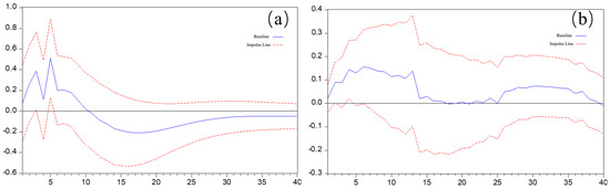
Figure 5.
Impulse response. (a) The impulse response of industrial growth rate to FCI. (b) The impulse response of price growth to FCI.
Moving forward, from Figure 5a, in the first nine periods, the response of financial sector growth rate to FCI’s impulse is positive. But, from the tenth stage, it is negative. This could reflect how the effect of financial expansion on output is a short-term stimulus which lasts for nine months. Then, it turns into a lasting restraint. From Figure 5b, the degree of the response of R_CPI to the impulse of a standard deviation from FCI1 varies in different periods, but it is a positive response from the beginning to the end. Among them, from the 1st period to the 14th period, the degree of response is relatively higher, and then gradually decays to zero. From the 25th period, the degree of response has increased gradually. This could demonstrate that the financial expansion can stimulate the price inflation for a long time, but the effect mainly focuses on the former 14 months.
6. Conclusions
6.1. Research Contributions
This study provides a systematic analysis of China’s financial cycle, integrating a dynamic weighting approach based on the Generalized Autoregressive Conditional Heteroskedasticity (GARCH) model, a Markov Switching (MS) model, and a Vector Autoregression (VAR) model. By constructing a Financial Conditions Index (FCI) with dynamically adjusted weights, this research offers a refined perspective on the measurement and characteristics of financial fluctuations in China, as well as their macroeconomic implications.
The findings highlight several key insights: (1) A more-accurate measurement of China’s financial cycle. Unlike previous studies that predominantly rely on fixed-weight methods, this study demonstrates that a dynamic weighting approach better reflects real-world financial fluctuations. By applying a GARCH-based dynamic weighting method, this research effectively captures the changing importance of financial indicators over time, addressing a key limitation in prior financial cycle measurements. This methodological refinement is particularly relevant in the context of China, where economic structure, financial regulations, and policy priorities evolve dynamically. (2) Identification of a four-phase financial cycle. By employing the MS model, this study identifies a four-zone financial cycle structure (boom, decline, depression, and recovery), a classification rarely applied to financial cycles in the existing literature. Prior studies (e.g., Deng & Xu, 2014; C. Borio, 2014) have typically focused on two-zone (expansion-contraction) or three-zone (tension-moderation-looseness) classifications. Our findings reveal that China’s financial cycle exhibits strong inertia, frequent imbalances, and a pronounced double asymmetry—characterized by fewer contractions but longer expansions. This distinction suggests that China’s financial cycle does not strictly conform to patterns observed in mature market economies, where financial contractions tend to be more frequent but shorter in duration. (3) Empirical evidence on the macroeconomic effects of financial cycles. Through the VAR model, we examine the macroeconomic effects of financial cycles and find that financial expansion stimulates output growth for approximately nine months before its effects begin to fade, whereas its impact on inflation is more prolonged, with the strongest effects occurring within the first 14 months. These findings not only offer a quantitative perspective on the lagged effects of financial cycles on macroeconomic variables but also reinforce the importance of proactive financial regulation in mitigating inflationary pressures and macroeconomic instability.
6.2. Research Limitations and Future Directions
Despite the contributions of this study, certain limitations should be acknowledged. First, while the dynamic weighting approach improves financial cycle measurement, it remains dependent on the selection of financial indicators, which may not fully capture all aspects of China’s financial conditions. Future research could explore alternative variable selection methods, such as incorporating high-frequency financial market data or leveraging machine learning techniques for enhanced weighting precision.
Second, although the MS model effectively captures the nonlinear characteristics of China’s financial cycle, its estimation relies on historical data, which may not fully account for structural shifts in China’s financial system. Expanding this framework to incorporate time-varying transition probabilities or state-dependent macroeconomic shocks could provide deeper insights into the dynamic interactions between financial and business cycles.
Third, this study primarily examines the financial cycle at the national level, yet regional disparities in financial development and policy responses may lead to heterogeneity in financial fluctuations. Future research could investigate regional financial cycles within China, assessing how financial conditions vary across different provinces or economic zones.
6.3. Policy Implications
The findings of this study carry significant policy implications. On the one hand, it demonstrates the need for macro-prudential financial regulation. Given the strong inertia and prolonged expansion phases of China’s financial cycle, policymakers must exercise caution in managing prolonged financial expansions, which can lead to excessive risk accumulation. Proactive macroprudential policies should be implemented to prevent financial overheating and ensure long-term stability.
On the other hand, the financial cycle can serve as an early warning indicator, ahead of output and price fluctuations, and evidence suggests that the inclusion of a financial volatility index in China’s macroeconomic policy framework can enhance the policy response to financial imbalances and can serve as a leading indicator of monetary policy adjustment.
Finally, the prolonged inflationary effects of financial expansion underscore the necessity for a balanced monetary policy that considers both short-term economic stimulus and long-term price stability. This highlights the importance of coordinating monetary and fiscal policies to achieve sustainable financial and economic development.
In conclusion, this study contributes to the literature by refining financial cycle measurement, offering new empirical insights into its macroeconomic effects, and providing a nuanced understanding of its nonlinear characteristics. While limitations exist, they also point to fruitful avenues for future research, particularly in refining financial cycle modeling and understanding regional financial dynamics. As China’s financial system continues to evolve, ongoing research in this area will remain essential for ensuring financial stability and sustainable economic growth.
Funding
This research received no external funding.
Informed Consent Statement
Not applicable.
Data Availability Statement
Data are available upon reasonable request.
Conflicts of Interest
The author declares no conflicts of interest. The funder had no role in the design of the study; in the collection, analyses, or interpretation of data; in the writing of the manuscript; or in the decision to publish the results.
References
- Aikman, D., Haldane, A. G., & Nelson, B. D. (2014). Curbing the credit cycle. The Economic Journal, 125, 1072–1109. [Google Scholar] [CrossRef]
- Angelopoulou, E., Balfoussia, H., & Gibson, H. D. (2014). Building a financial conditions index for the euro area and selected euro area countries: What does it tell us about the crisis? Economic Modelling, 38, 392–403. [Google Scholar] [CrossRef]
- Balfoussia, H., Burlon, L., Buss, G., Comunale, M., Backer, B. D., Dewachter, H., Guarda, P., Haavio, M., & Hindrayanto, I. (2018). Real and financial cycles in eu countries: Stylised facts and modelling implications. ECBS Occasional Papers, Eesti Pank. [Google Scholar]
- Bollerslev, T. (1986). Generalized auto-regressive conditional heteroscedasticity. Journal of Econometrics, 31, 307–327. [Google Scholar] [CrossRef]
- Borio, C. (2014). The financial cycle and macroeconomics: What have we learnt? Journal of Banking & Finance, 45, 182–198. [Google Scholar] [CrossRef]
- Borio, C. E., Drehmann, M., & Xia, F. D. (2019). Predicting recessions: Financial cycle versus term spread. Bank for International Settlements. [Google Scholar]
- Burns, A. F., & Mitchell, W. C. (1946). Measuring business cycles. National Bureau of Economic Research. [Google Scholar]
- Chen, X., & Zhang, F. (2017). Study on financial cycle convergence between china and east Asian and southeast Asian countries and regions. Studies of International Finance, 11, 3–12. [Google Scholar]
- Chen, Y., & Ma, Y. (2013). Dajinrong lungang. Renmin University of China Press. [Google Scholar]
- Claessens, S., Kose, M. A., & Terrones, M. E. (2012). How do business and financial cycles interact? Journal of International Economics, 87, 178–190. [Google Scholar] [CrossRef]
- Deng, C., Teng, L., & Xu, M. (2016). Analysis of the fluctuation characteristics and its macroeconomic effects of china’s financial situation. Studies of International Finance, 3, 17–27. [Google Scholar]
- Deng, C., & Xu, M. (2014). Financial cycle fluctuation and its macro economic effects. Studies of Quantitative Economy and Technical Economy, 9, 75–91. [Google Scholar]
- Drehmann, M., Borio, C., & Tsatsaronis, K. (2012). Characterising the financial cycle: Don’t lose sight of the medium term! Bank for International Settlements. [Google Scholar]
- Drehmann, M., & Yetman, J. (2018). Why you should use the hodrick-prescott filter——At least to generate credit gaps. Bank for International Settlements. [Google Scholar]
- Dudley, W., & Hatzius, J. (2000). The goldman sachs financial conditions index: The right tool for a new monetary policy regime. Goldman Sachs. [Google Scholar]
- Fan, X., Yuan, M., & Xiao, L. (2017). Understanding china’s financial cycle: Theory, measurement and analysis. Studies of International Finance, 1, 28–38. [Google Scholar]
- Feng, S., Jiang, F., Xie, Q., & Zhang, W. (2012). Mechanism and empirical analysis of inflation trends forecasting by financial conditions index. China Industrial Economics, 4, 18–30. [Google Scholar]
- Gauthier, C., Graham, C., & Liu, Y. (2004). Financial conditions indices for Canada. Bank of Canada. [Google Scholar]
- Goodhart, C., & Hofmann, B. (2001, March 2–3). Asset prices, financial conditions and the transmission of monetary policy. Conference on Asset Prices, Exchange Rates and Monetary Policy, Stanford, CA, USA. [Google Scholar]
- Hamilton, J. D. (1989). A new approach to the economic analysis of nonstationary time series and the business cycle. Econometrica, 57, 357–384. [Google Scholar] [CrossRef]
- Han, T. (2018). A comparative study of international convergence in financial cycles. Inquiry into Economic Issues, 10, 130–139. [Google Scholar]
- Hardana, A., Windari, W., Efendi, S., & Harahap, H. T. (2023). Comparing credit procyclicality in conventional and Islamic rural banks: Evidence from Indonesia. In Annual international conference on islamic economics and business (Vol. 3, pp. 188–197). Faculty of Islamic Economics and Business (FEBI) & State Institute for Islamic Studies (IAIN) Salatiga. [Google Scholar]
- Jabeenm, H., & Qureshi, M. N. (2019). Financial condition index (FCI) for the Pakistan. Indian Journal of Science and Technology, 12(21), 1–8. [Google Scholar] [CrossRef]
- Koop, G., & Korobilis, D. (2014). A new index of financial conditions. European Economic Review, 71, 101–116. [Google Scholar] [CrossRef]
- Liu, Y., & Li, N. (2018). The construction of china’s financial condition index in post crisis era. Economic Theory and Business Management, 1, 46–60. [Google Scholar] [CrossRef]
- Lu, J., & Liang, J. (2007). The construction of china’s financial condition index. The Journal of World Economy, 3, 36–52. [Google Scholar]
- Lu, X., Wang, P., & Hou, C. (2024). The financial cycle in China: Index construction and its interaction with the economic cycle. Management Review, 11, 50–60. [Google Scholar]
- Ma, Y., & Zhang, J. (2016). Financial cycle, business cycle and monetary policy: Evidence from four major economies. International Journal of Finance & Economics, 21, 502–527. [Google Scholar] [CrossRef]
- Miao, W., Zhong, S., & Zhou, C. (2018). Financial cycle, industrial technology fluctuation and economic structure optimization. Journal of Financial Research, 3, 36–52. [Google Scholar]
- Minsky, H. P. (1977). The financial instability hypothesis: An interpretation of Keynes and an alternative to “standard” theory. Nebraska Journal of Economics & Business, 16, 5–16. [Google Scholar]
- Nakajima, J., Kasuya, M., & Watanabe, T. (2011). Bayesian analysis of time-varying parameter vector autoregressive model for the Japanese economy and monetary policy. Journal of the Japanese and International Economies, 25, 225–245. [Google Scholar] [CrossRef]
- Niemira, M. P., & Klein, P. A. (1994). Forecasting financial and economic cycles. John Wiley & Sons. [Google Scholar]
- Praet, P. (2016). Financial cycles and monetary policy. European Central Bank: Speech Given at the Panel on International Monetary Policy, Beijing. [Google Scholar]
- Schüler, Y. S., Hiebert, P. P., & Peltonen, T. A. (2015). Characterising the financial cycle: A multivariate and time-varying approach. German National Library of Economics, Leibniz Information Centre for Economics. [Google Scholar]
- Sun, T., Wang, X., & Shang, X. (2020). A structural perspective on the procyclicality of cross-border capital flows. Finance & Trade Economics, 41, 70–85. [Google Scholar]
- Swiston, A. J. (2008). A U.S. financial conditions index putting credit where credit is due (WP/08/161). International Monetary Fund. [Google Scholar]
- Tian, X., Jacobs, J. P., & de Haan, J. (2024). Alternative measures for the global financial cycle: Do they make a difference? International Journal of Finance & Economics, 29(4), 4483–4498. [Google Scholar]
- Vonen, N. H. (2011). A financial conditions index for Norway. Norges Bank. [Google Scholar]
- Wang, C., Chen, L., & Li, Y. (2020). Characteristics of China’s financial cycle and its macroeconomic effects. Chinese Management Science, 12, 12–22. [Google Scholar]
- Wang, Y. (2005). An empirical analysis of china’s financial condition index. Shanghai Finance, 8, 29–32. [Google Scholar]
- Xiong, Y., & Zhang, Z. (2018). China-macro: Launching a financial conditions index (FCI) for China. Deutsche Bank Market Research. [Google Scholar]
- Yao, D., Shi, T., & Liu, Z. (2021). The state transition effect of systemic financial risk in China from the perspective of the financial cycle. Journal of Financial Economics, 2, 3–17. [Google Scholar]
- Yi, N., & Zhang, B. (2016). Measuring China’s financial cycle. Studies of International Finance, 6, 13–23. [Google Scholar]
- Zhu, T., & Huang, H. (2018). China’s financial cycle: Indicators, methods and empirical research. Journal of Financial Research, 12, 55–71. [Google Scholar]


Disclaimer/Publisher’s Note: The statements, opinions and data contained in all publications are solely those of the individual author(s) and contributor(s) and not of MDPI and/or the editor(s). MDPI and/or the editor(s) disclaim responsibility for any injury to people or property resulting from any ideas, methods, instructions or products referred to in the content. |
© 2025 by the author. Licensee MDPI, Basel, Switzerland. This article is an open access article distributed under the terms and conditions of the Creative Commons Attribution (CC BY) license (https://creativecommons.org/licenses/by/4.0/).