Figure 1.
GARCH-XGBoost diagram workflow.
Figure 1.
GARCH-XGBoost diagram workflow.
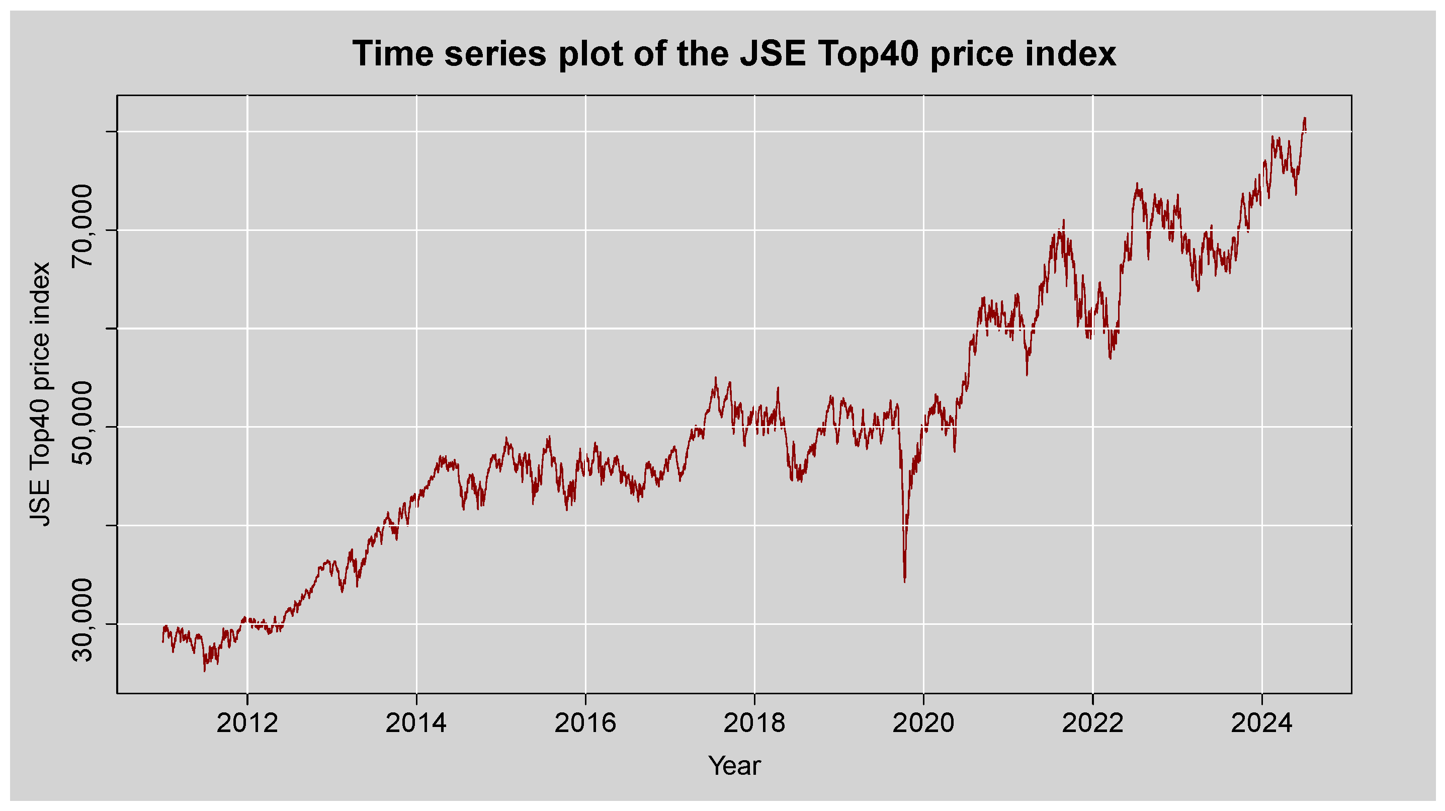
Figure 2.
Time series plot of the JSE Top40 Price Index.
Figure 2.
Time series plot of the JSE Top40 Price Index.
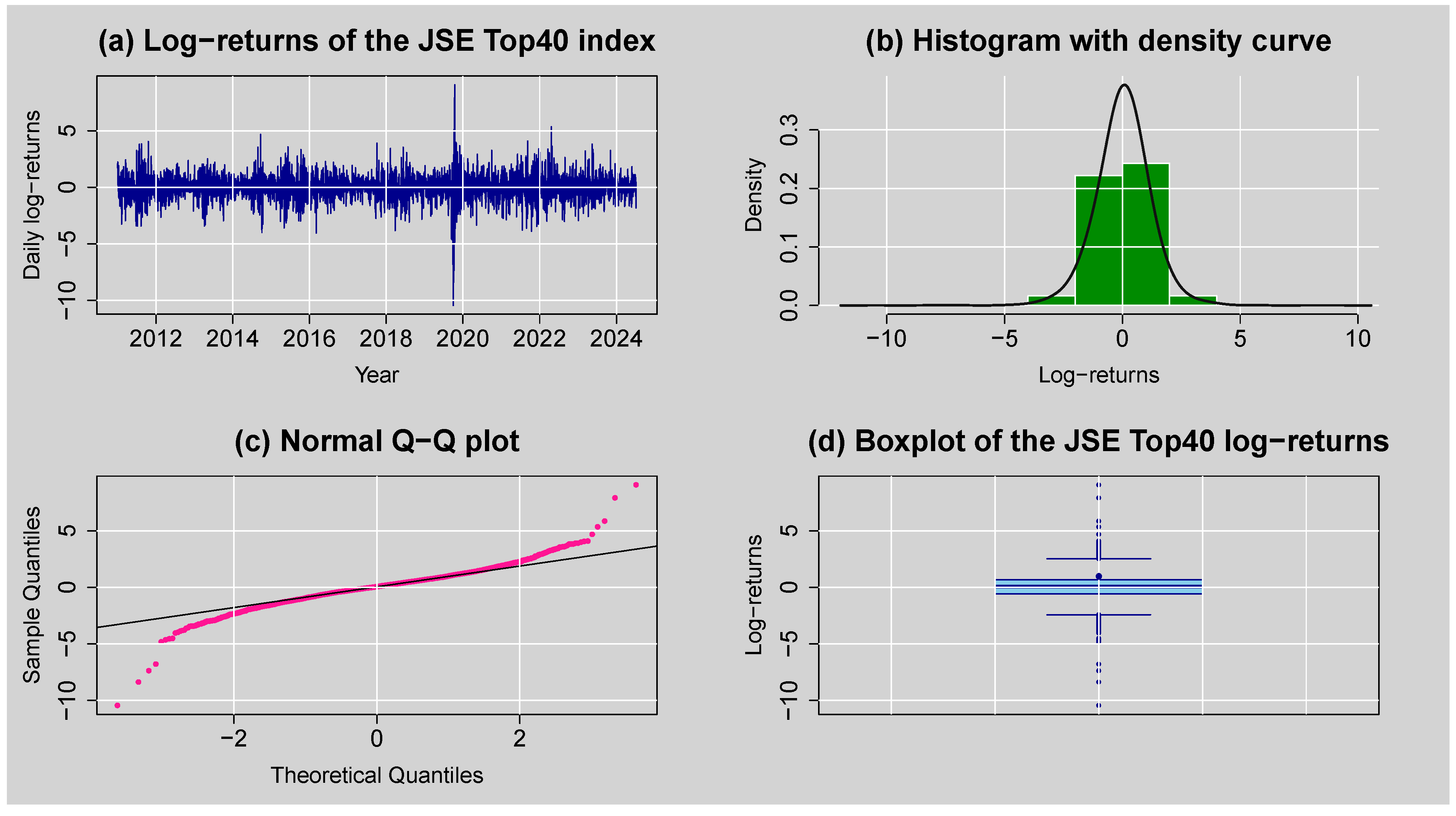
Figure 3.
(a) Log-returns for JSE Top40 stock index, (b) histogram with density curve plot of daily log-returns, (c) normal Q–Q plot of daily log-returns, and (d) boxplot of the JSE Top40 log-returns.
Figure 3.
(a) Log-returns for JSE Top40 stock index, (b) histogram with density curve plot of daily log-returns, (c) normal Q–Q plot of daily log-returns, and (d) boxplot of the JSE Top40 log-returns.
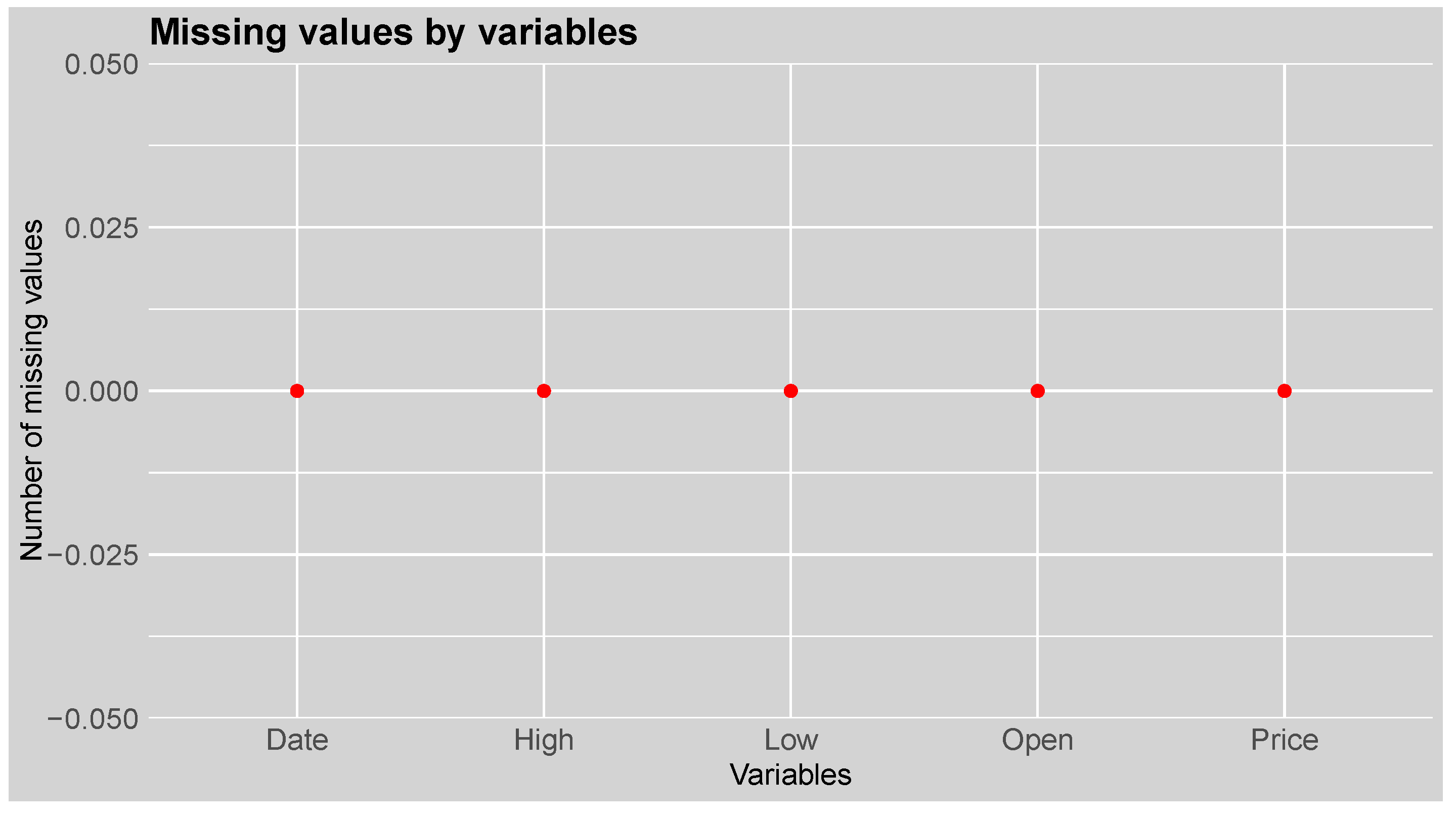
Figure 4.
Missing value plot of each variable of the JSE Top40 index.
Figure 4.
Missing value plot of each variable of the JSE Top40 index.
Figure 5.
ACF and PACF plots of the standardised JSE Top40 log-returns.
Figure 5.
ACF and PACF plots of the standardised JSE Top40 log-returns.
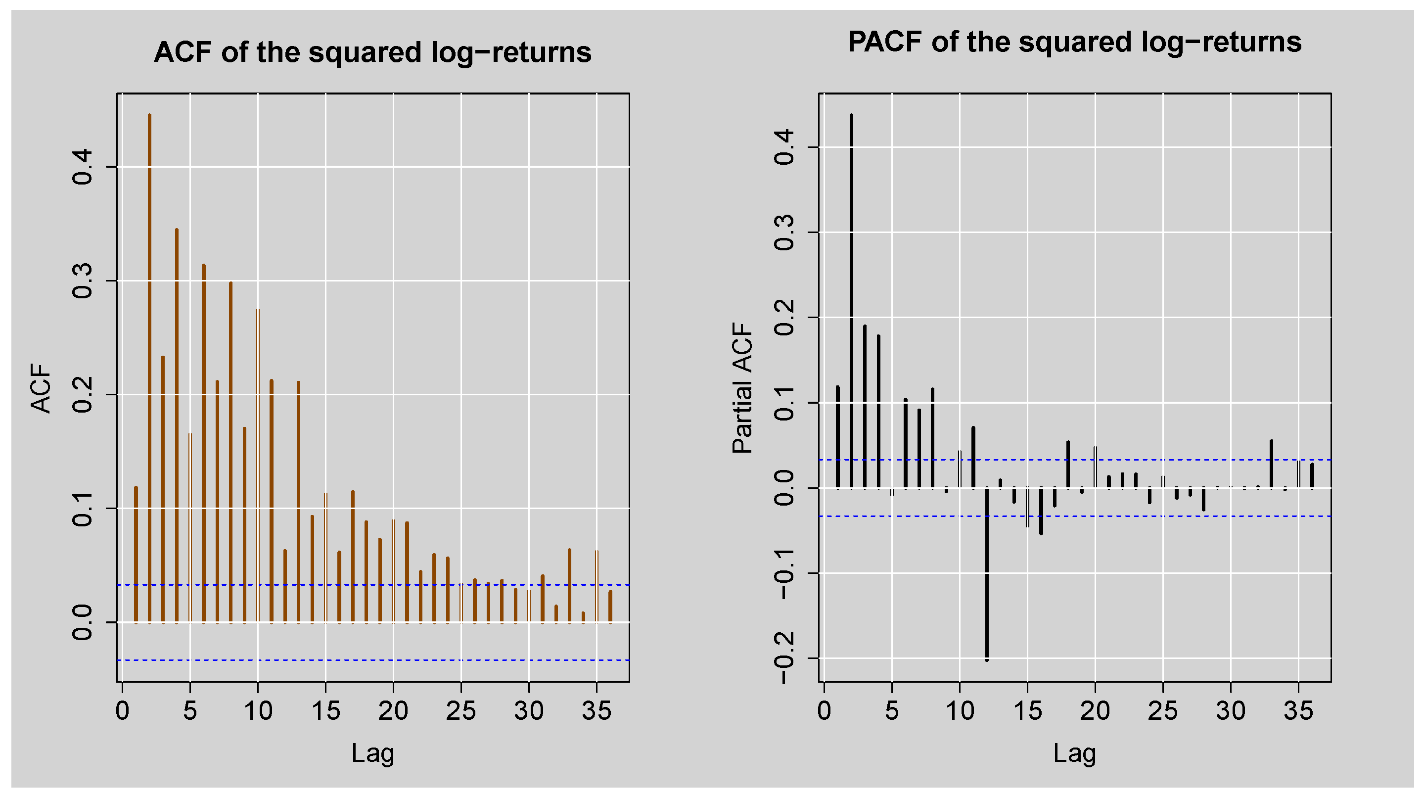
Figure 6.
ACF and PACF plots of the squared standardised JSE Top40 log-returns.
Figure 6.
ACF and PACF plots of the squared standardised JSE Top40 log-returns.
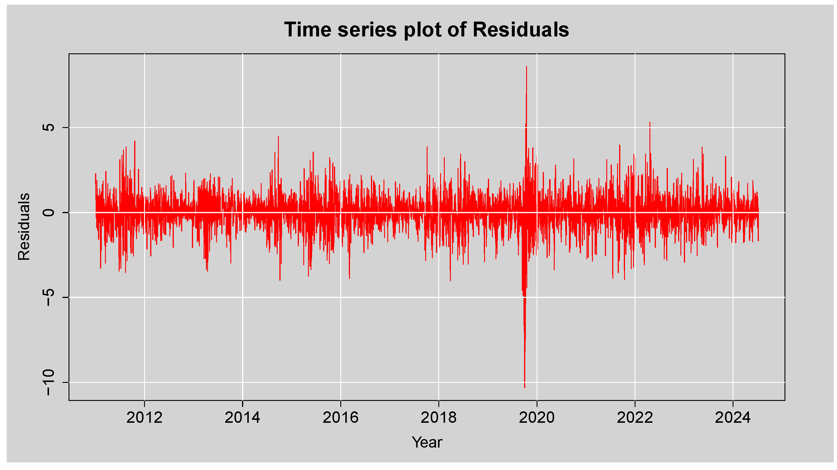
Figure 7.
Time series plot of the Residuals from ARMA (3,2) model.
Figure 7.
Time series plot of the Residuals from ARMA (3,2) model.
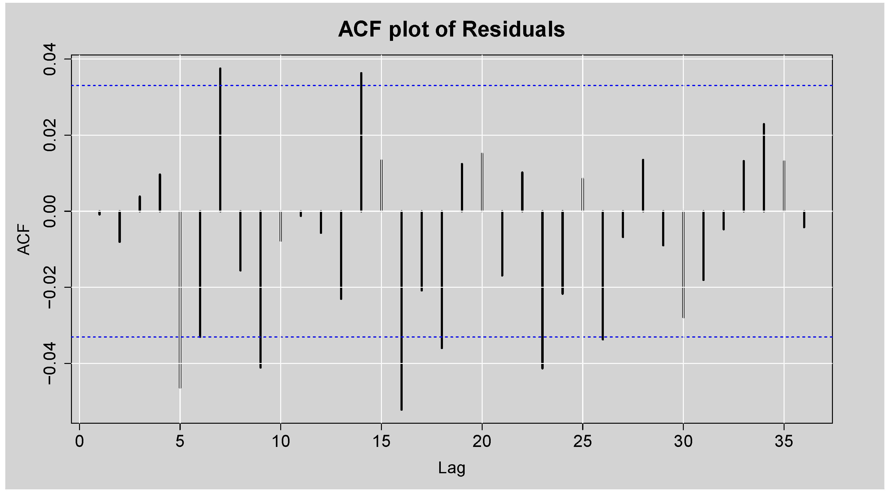
Figure 8.
ACF and PACF plots of the Residuals from ARMA(3,2) model.
Figure 8.
ACF and PACF plots of the Residuals from ARMA(3,2) model.
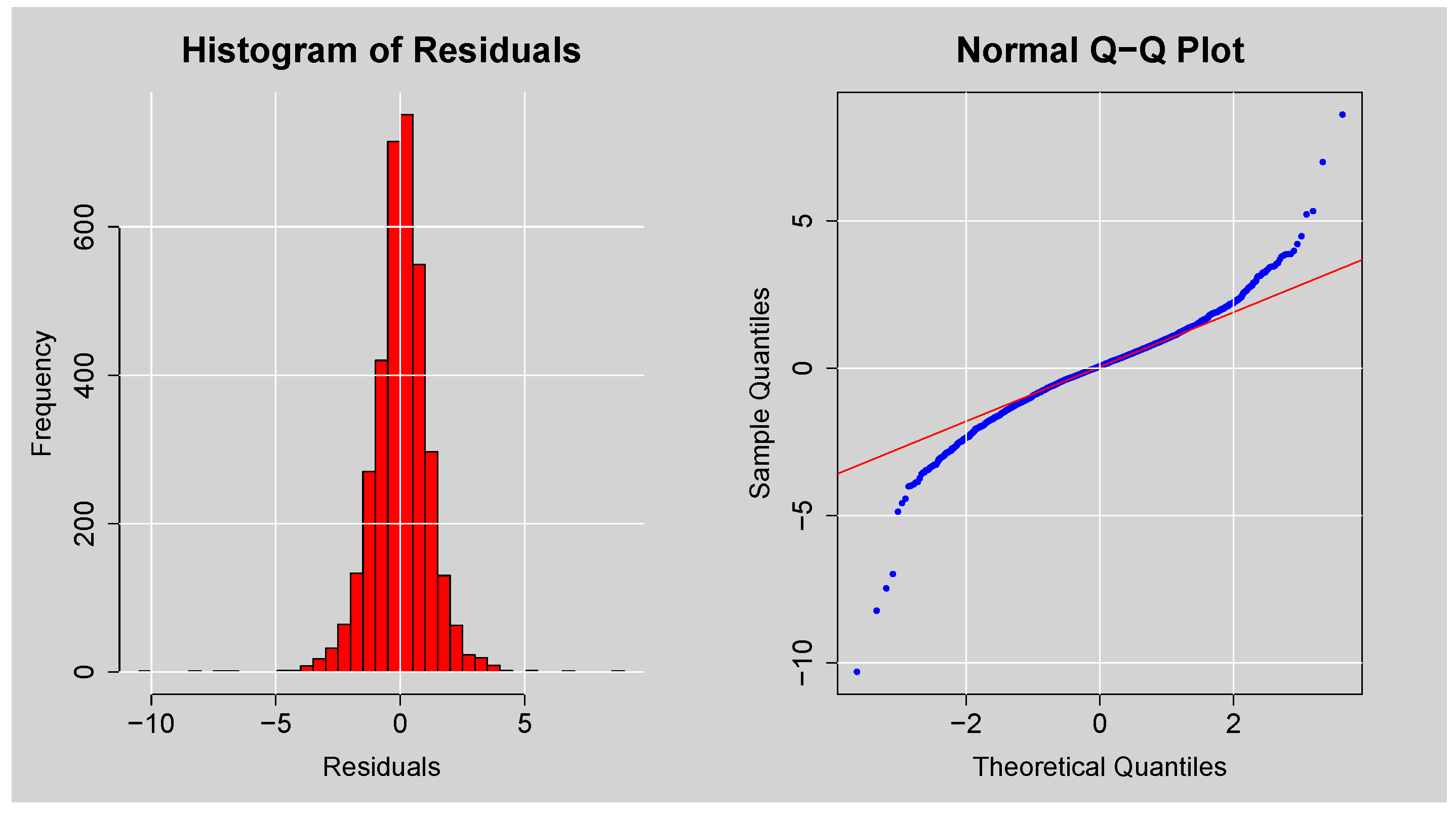
Figure 9.
Histogram and Normal Q-Q plots of the Residuals from ARMA(3,2) model.
Figure 9.
Histogram and Normal Q-Q plots of the Residuals from ARMA(3,2) model.
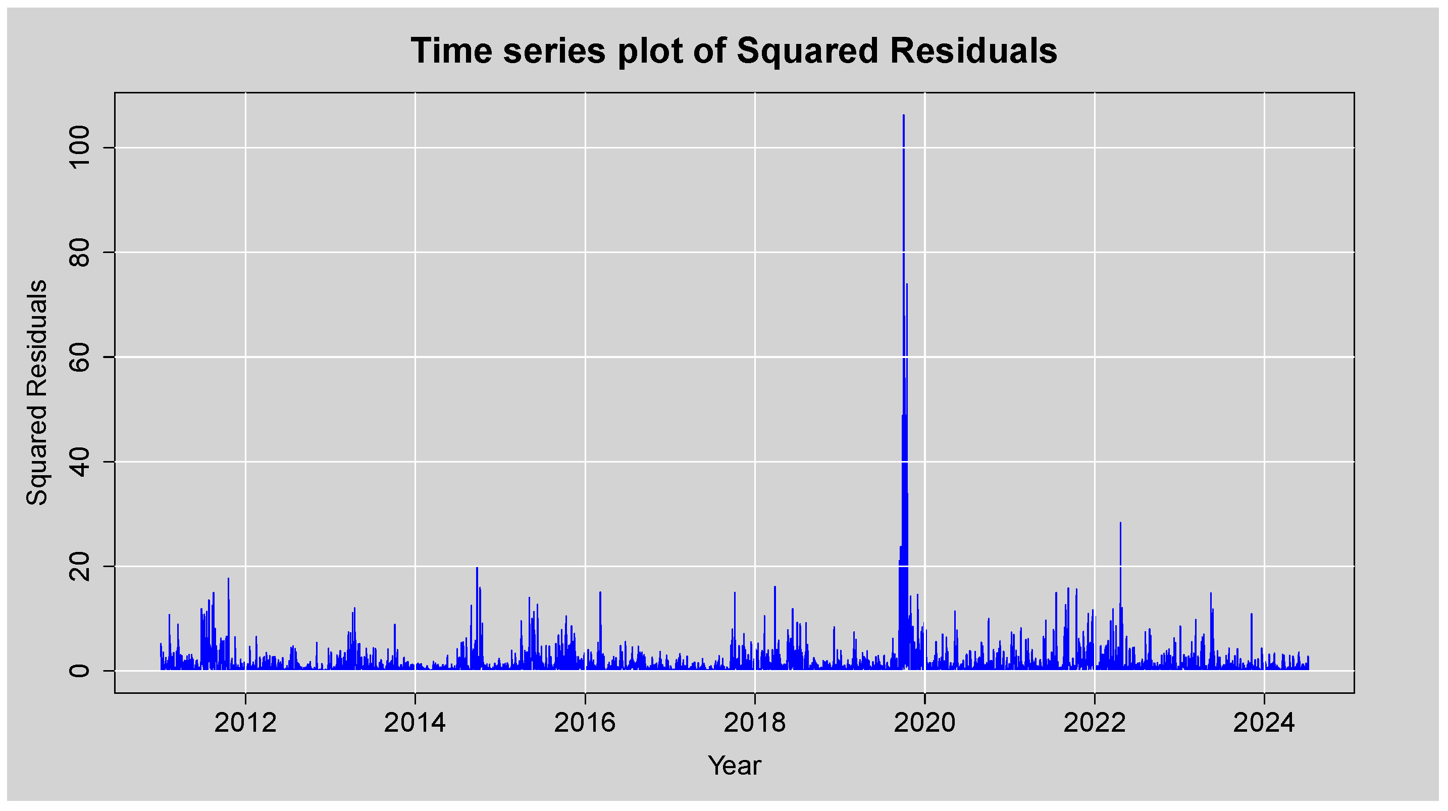
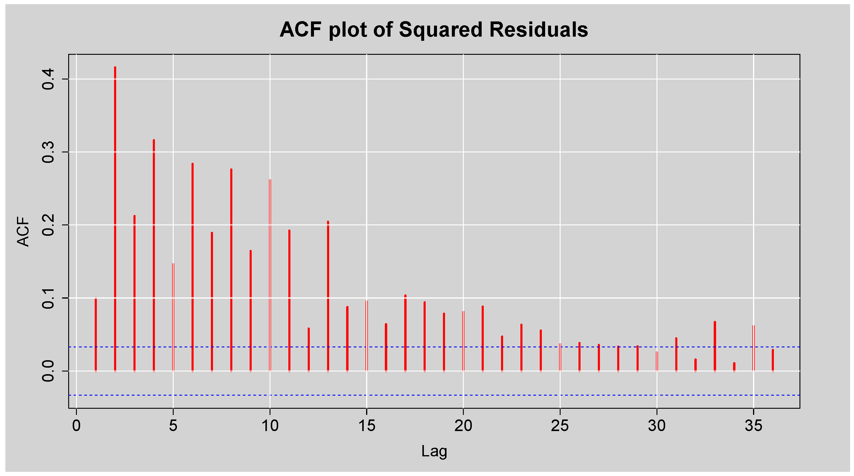
Figure 10.
Time series plot of the Squared Residuals from ARMA(3,2) model.
Figure 10.
Time series plot of the Squared Residuals from ARMA(3,2) model.
Figure 11.
ACF plot of the Squared Residuals from ARMA(3,2) model.
Figure 11.
ACF plot of the Squared Residuals from ARMA(3,2) model.
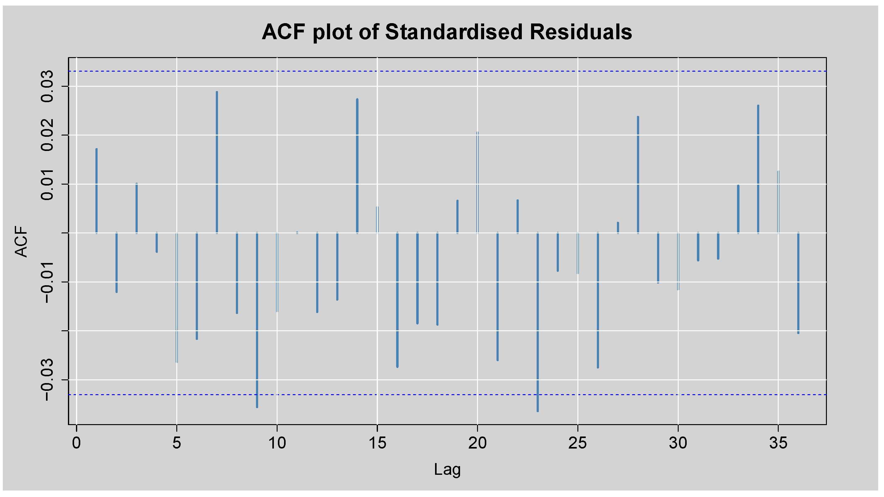
Figure 12.
ACF plot of the Standardised Residuals from ARMA(3,2)-EGARCH(1,1) model.
Figure 12.
ACF plot of the Standardised Residuals from ARMA(3,2)-EGARCH(1,1) model.
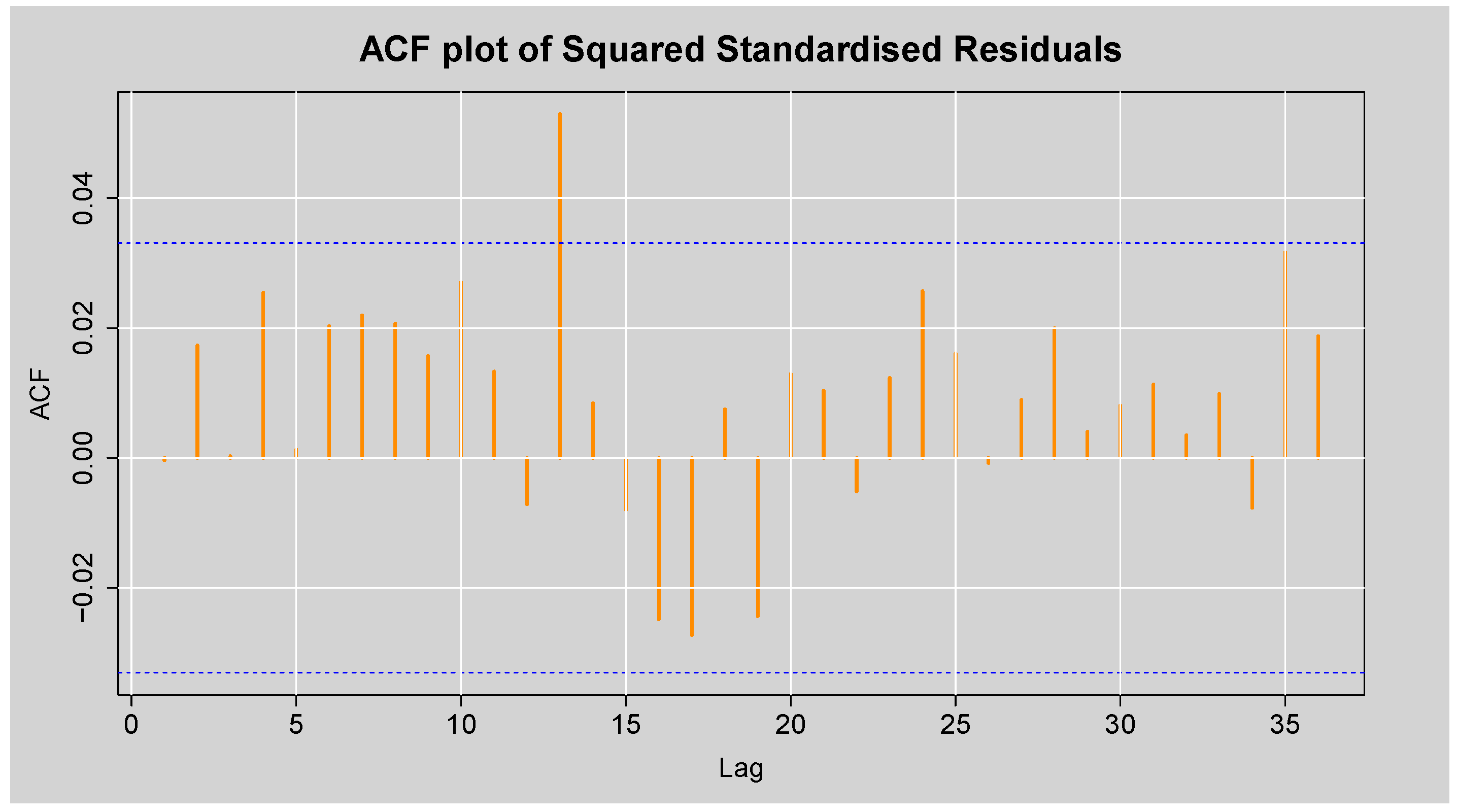
Figure 13.
ACF plot of the Squared Standardised Residuals from ARMA(3,2)-EGARCH(1,1) model.
Figure 13.
ACF plot of the Squared Standardised Residuals from ARMA(3,2)-EGARCH(1,1) model.
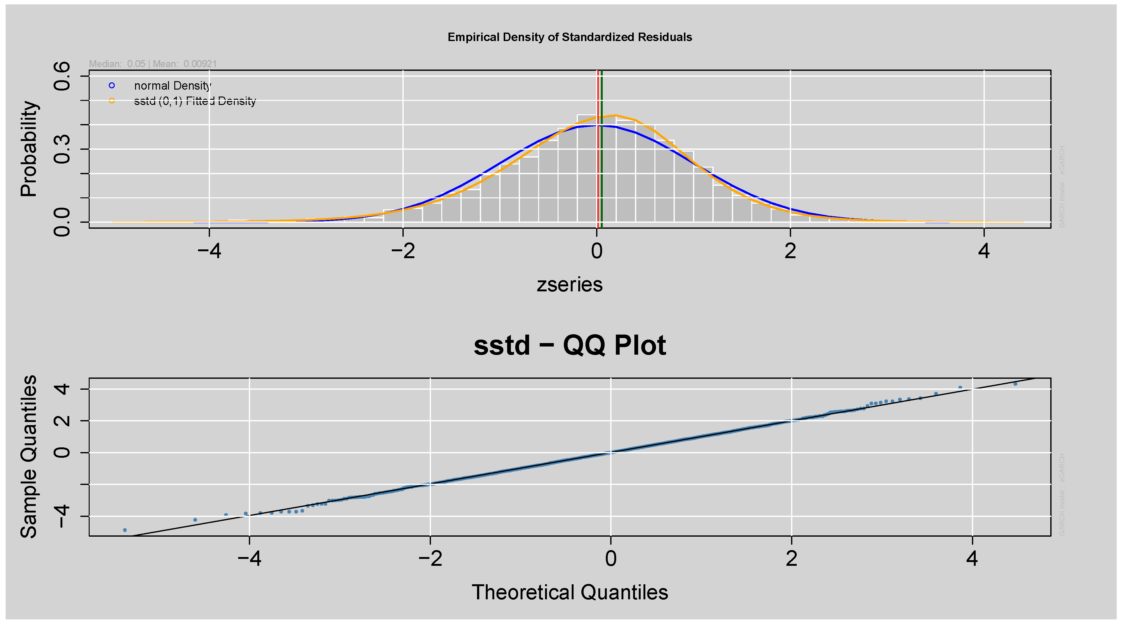
Figure 14.
Q-Q and Empirical Density plots of the Standardised Residuals from ARMA(3,2)-EGARCH(1,1) model.
Figure 14.
Q-Q and Empirical Density plots of the Standardised Residuals from ARMA(3,2)-EGARCH(1,1) model.
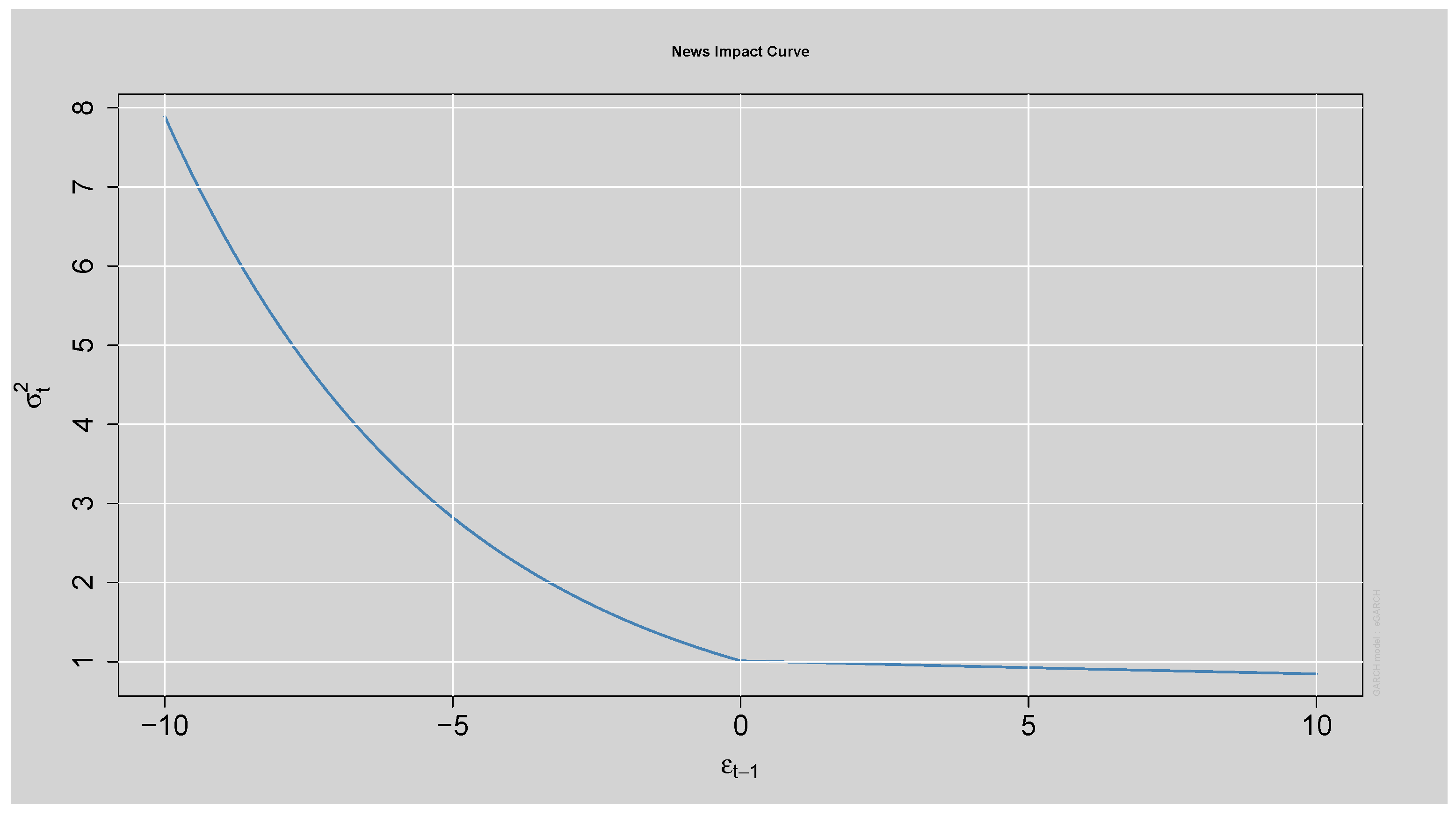
Figure 15.
News Impact Curve.
Figure 15.
News Impact Curve.
Figure 16.
Forecast of Standardised Residuals with 90% Prediction Intervals from the ARMA(3,2)-EGARCH(1,1)-XGBoost Model.
Figure 16.
Forecast of Standardised Residuals with 90% Prediction Intervals from the ARMA(3,2)-EGARCH(1,1)-XGBoost Model.
Figure 17.
Forecast of Standardised Residuals with 95% Prediction Intervals from the ARMA(3,2)-EGARCH(1,1)-XGBoost Model.
Figure 17.
Forecast of Standardised Residuals with 95% Prediction Intervals from the ARMA(3,2)-EGARCH(1,1)-XGBoost Model.
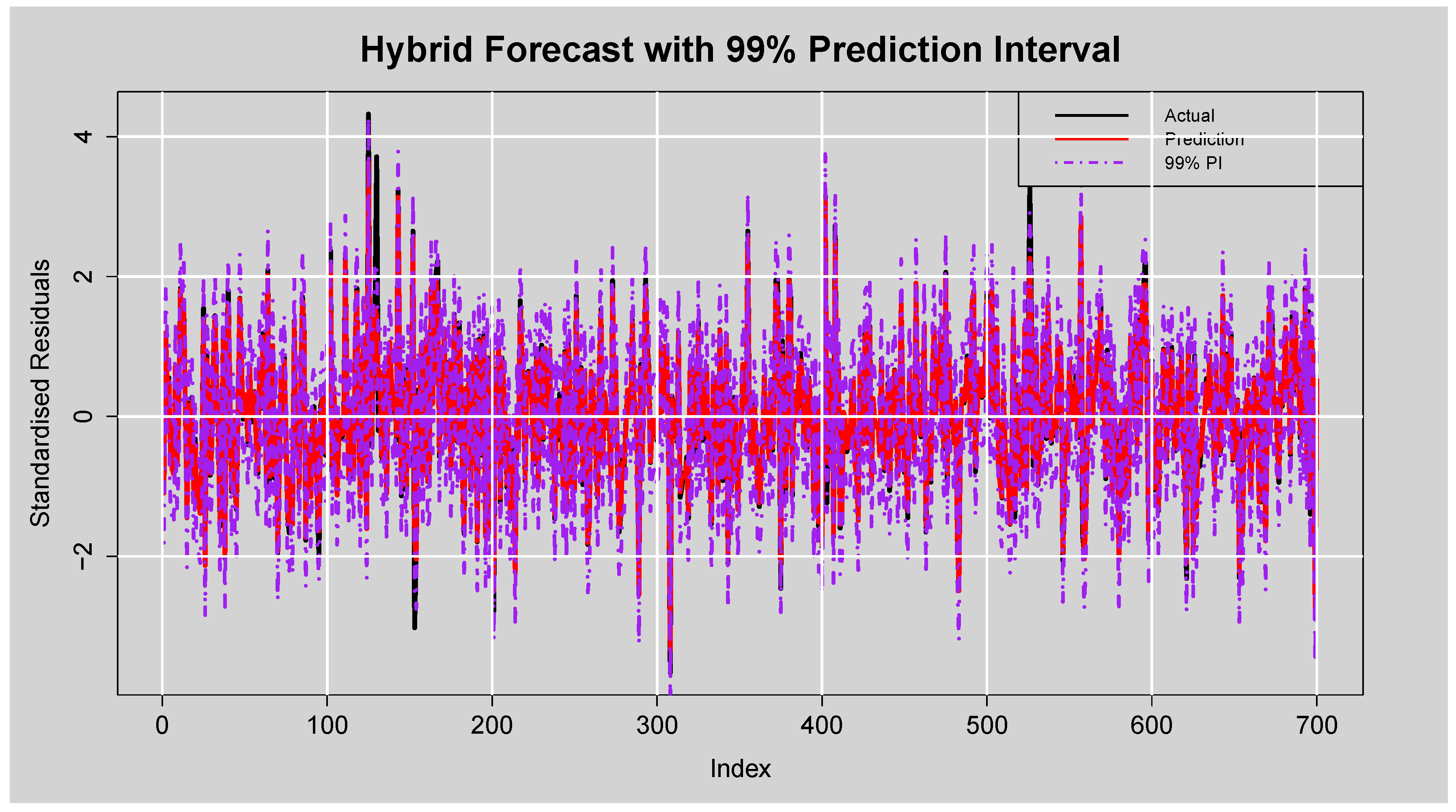
Figure 18.
Forecast of Standardised Residuals with 99% Prediction Intervals from the ARMA(3,2)-EGARCH(1,1)-XGBoost Model.
Figure 18.
Forecast of Standardised Residuals with 99% Prediction Intervals from the ARMA(3,2)-EGARCH(1,1)-XGBoost Model.
Figure 19.
Time-Varying Forecast Errors plot.
Figure 19.
Time-Varying Forecast Errors plot.
Table 1.
Results of the Box-Ljung Q test for autocorrelation detection.
Table 1.
Results of the Box-Ljung Q test for autocorrelation detection.
| Lag | Statistic | Critical Value | p-Value |
|---|
| 10 | | | |
| 15 | | | |
| 20 | | | |
| 25 | | | |
| 30 | | | |
| 35 | | | |
Table 2.
Results of the Engle’s ARCH LM test for heteroscedasticity detection.
Table 2.
Results of the Engle’s ARCH LM test for heteroscedasticity detection.
| Lag | Statistic | Critical Value | p-Value |
|---|
| 10 | | | <2.2 |
| 15 | | | <2.2 |
| 20 | | | <2.2 |
| 25 | | | <2.2 |
| 30 | | | <2.2 |
| 35 | | | <2.2 |
Table 3.
Summary of stationarity and normality tests for the log-returns.
Table 3.
Summary of stationarity and normality tests for the log-returns.
| Test | Statistic | p-Value | Conclusion | Decision |
|---|
| ADF | | | Reject H0 | Stationary |
| KPSS | | | Fail to reject H0 | Stationary |
| JB | | <2.2 | Reject H0 | Not normally distributed |
Table 4.
Summary statistics of the log-returns.
Table 4.
Summary statistics of the log-returns.
| Min | Q1 | Q2 | Mean | Q3 | Max | SD | Skew | Kurt |
|---|
| | | | | | | | |
Table 5.
Box-Lyung and JB test on the ARMA(3,2) Residuals.
Table 5.
Box-Lyung and JB test on the ARMA(3,2) Residuals.
| Lag | Statistic | p-Value |
|---|
| 10 | | |
| 15 | | |
| 20 | | |
| 25 | | |
| 30 | | |
| 30 | | |
| | <2.2 |
Table 6.
Engle’s ARCH LM test on the ARMA(3,2) Residuals.
Table 6.
Engle’s ARCH LM test on the ARMA(3,2) Residuals.
| Lag | Statistic | p-Value |
|---|
| 10 | | <2.2 |
| 15 | | <2.2 |
| 20 | | <2.2 |
| 25 | | <2.2 |
| 30 | | <2.2 |
Table 7.
Box-Ljung test on the ARMA(3,2) Squared Residuals.
Table 7.
Box-Ljung test on the ARMA(3,2) Squared Residuals.
| Lag | Statistic | p-Value |
|---|
| 10 | | <2.2 |
| 15 | | <2.2 |
| 20 | | <2.2 |
| 25 | | <2.2 |
| 30 | | <2.2 |
Table 8.
Evaluation metrics for ARMA(3,2)–GARCH-type models under different conditional distributions.
Table 8.
Evaluation metrics for ARMA(3,2)–GARCH-type models under different conditional distributions.
| | Conditional Distributions |
|---|
| Model | | STD | SSTD | GED | SGED | GHD |
|---|
| ARMA(3,2)-sGARCH(1,1) | AIC | | | | | |
| | BIC | | | | | |
| | HQIC | | | | | |
| | LL | | | | | |
| ARMA(3,2)-EGARCH(1,1) | AIC | | | | | |
| | BIC | | | | | |
| | HQIC | | | | | |
| | LL | | | | | |
| ARMA(3,2)-GJR-GARCH(1,1) | AIC | | | | | |
| | BIC | | | | | |
| | HQIC | | | | | |
| | LL | | | | | |
Table 9.
Box-Lyung test on the ARMA(3,2)-EGARCH(1,1) Standardised Residuals.
Table 9.
Box-Lyung test on the ARMA(3,2)-EGARCH(1,1) Standardised Residuals.
| Lag | Statistic | p-Value |
|---|
| 1 | | |
| 14 | | |
| 24 | | |
Table 10.
Engle’s ARCH LM test on the ARMA(3,2)-EGARCH(1,1) Standardised Residuals.
Table 10.
Engle’s ARCH LM test on the ARMA(3,2)-EGARCH(1,1) Standardised Residuals.
| Lag | Statistic | p-Value |
|---|
| 3 | | |
| 5 | | |
| 7 | | |
Table 11.
Box-Ljung test on the ARMA(3,2)-EGARCH(1,1) Squared Standardised Residuals.
Table 11.
Box-Ljung test on the ARMA(3,2)-EGARCH(1,1) Squared Standardised Residuals.
| Lag | Statistic | p-Value |
|---|
| 1 | | |
| 5 | | |
| 9 | | |
Table 12.
Sign Bias Test Results.
Table 12.
Sign Bias Test Results.
| | t-Value | p-Value |
|---|
| Sign Bias | | |
| Negative Sign Bias | | |
| Positive Sign Bias | | |
| Joint Effect | | |
Table 13.
Parameter Estimates of the ARMA(3,2)-EGARCH(1,1) model.
Table 13.
Parameter Estimates of the ARMA(3,2)-EGARCH(1,1) model.
| Parameter | Estimate | p-Value |
|---|
| | |
| | |
| | |
| | |
| | |
Table 14.
First 10 Forecast Results from the Hybrid ARMA(3,2)-EGARCH(1,1)-XGBoost Model.
Table 14.
First 10 Forecast Results from the Hybrid ARMA(3,2)-EGARCH(1,1)-XGBoost Model.
| Actual | Prediction |
|---|
| |
| |
| |
| |
| |
| |
| |
| |
| |
| |
Table 15.
Forecast Accuracy Measure Results from the Hybrid ARMA(3,2)-EGARCH(1,1)-XGBoost Model.
Table 15.
Forecast Accuracy Measure Results from the Hybrid ARMA(3,2)-EGARCH(1,1)-XGBoost Model.
| Forecast Accuracy Measures |
|---|
| MASE | RMSE | MAE | MAPE (%) | sMAPE (%) |
| | | | |
Table 16.
Evaluation Metrics of the Prediction Intervals.
Table 16.
Evaluation Metrics of the Prediction Intervals.
| Evaluation Metrics |
|---|
| PINC (%) | PICP (%) | PINAW (%) | PICAW (%) | PINAD (%) |
|---|
| | | | |
| | | | |
| | | | |
Table 17.
Forecast Accuracy Measures for ARMA(3,2)-EGARCH(1,1) and ARMA(3,2)-EGARCH(1,1)-XGBoost Models.
Table 17.
Forecast Accuracy Measures for ARMA(3,2)-EGARCH(1,1) and ARMA(3,2)-EGARCH(1,1)-XGBoost Models.
| Accuracy Measure | ARMA(3,2)-EGARCH(1,1) | ARMA(3,2)-EGARCH(1,1)-XGBoost |
|---|
| MASE | 0.6827 | 0.0534 |
| RMSE | 1.0845 | 0.1386 |
| MAE | 0.8176 | 0.0595 |
| MAPE (%) | 165.182 | 27.9251 |
| sMAPE (%) | 177.287 | 16.4121 |

