Article

Exchange Rate Forecasting: A Deep Learning Framework Combining Adaptive Signal Decomposition and Dynamic Weight Optimization

School of Business, Jiangnan University, Wuxi 214122, China
*
Author to whom correspondence should be addressed.
Int. J. Financial Stud. 2025, 13(3), 151; https://doi.org/10.3390/ijfs13030151
Submission received: 14 July 2025 / Revised: 14 August 2025 / Accepted: 18 August 2025 / Published: 22 August 2025

Abstract

Accurate exchange rate forecasting is crucial for investment decisions, multinational corporations, and national policies. The nonlinear nature and volatility of the foreign exchange market hinder traditional forecasting methods in capturing exchange rate fluctuations. Despite advancements in machine learning and signal decomposition, challenges remain in high-dimensional data handling and parameter optimization. This study mitigates these constraints by introducing an innovative enhanced prediction framework that integrates the optimal complete ensemble empirical mode decomposition with adaptive noise (OCEEMDAN) method and a strategically optimized combination weight prediction model. The grey wolf optimizer (GWO) is employed to autonomously modify the noise parameters of OCEEMDAN, while the zebra optimization algorithm (ZOA) dynamically fine-tunes the weights of predictive models—Bi-LSTM, GRU, and FNN. The proposed methodology exhibits enhanced prediction accuracy and robustness through simulation experiments on exchange rate data (EUR/USD, GBP/USD, and USD/JPY). This research improves the precision of exchange rate forecasts and introduces an innovative approach to enhancing model efficacy in volatile financial markets.

1. Introduction

In recent years, the rise of global tariff barriers and frequent adjustments to trade policies have had a noticeable impact on exchange rate markets. The United States, the European Union, and several East Asian economies have increased import tariffs in key industries, raising concerns about the outlook for international trade. This has caused noticeable fluctuations in some currencies, especially in emerging Asian markets, reflecting the sensitivity of exchange rates to trade costs. Increased volatility has added uncertainty to foreign exchange markets and raised the risks of cross-border trade and investment. As globalization continues, exchange rates remain a key link between national economies (S. Liu et al., 2024). They reflect macroeconomic fundamentals and influence the stability of capital flows and international transactions. Therefore, analyzing exchange rate dynamics and forecasting trends is essential for investors and multinational firms to make informed decisions and manage risks effectively (Alexandridis et al., 2024).
However, due to the complexity and dynamic nature of the foreign exchange market, exchange rate data exhibit distinct characteristics, such as nonlinearity, nonstationarity, and high volatility, making accurate prediction of exchange rate fluctuations extremely challenging (Semenov, 2024). Exchange rate fluctuations are influenced by domestic and international economic conditions, global market sentiment, politics, and other external factors. Factors such as market participants’ psychological expectations, political conflicts, and financial crises often have a significant impact on exchange rates, further complicating the exchange rate data (P. Liu et al., 2023). Therefore, designing a forecasting method that can effectively address the complexity of exchange rate fluctuations has become a critical challenge in both academic research and financial practice. Exchange rates are not merely time series data but also involve multidimensional factors such as international capital flows and differences in monetary policies between countries. Extracting valuable signals from these complex factors is key to improving the accuracy and stability of predictions.
To address the complexity of exchange rate fluctuations, this paper introduces an innovative intelligent forecasting framework that combines optimal signal decomposition with multiple deep learning models. The GWO is used to optimize noise parameters in the decomposition process, enhancing accuracy and stability. Unlike traditional methods, this study employs Bi-LSTM, GRU, and FNN to model the decomposed subsequences and integrates their predictions using the ZOA. To adapt to market changes, this method dynamically adjusts combination weights, leveraging the complementary advantages of each model. This adaptation to varying market conditions significantly improves forecasting accuracy and robustness.
This study is structured as follows: Section 2 reviews key literature on exchange rate forecasting. Section 3 outlines the methodology and core techniques of the model. Section 4 describes the model’s structure and evaluation metrics. Section 5 conducts an empirical analysis and compares forecasting performance. Section 6 concludes with the main findings.

2. Literature Review

Forecasting exchange rates poses significant challenges due to their inherent nonlinearity and the impact of multiple external influences. The intricate behavior of currency fluctuations has led to the development of various predictive strategies, generally grouped into three types: traditional statistical techniques, artificial intelligence-based methods, and integrated hybrid systems. Statistical approaches typically rely on linear frameworks, whereas AI-driven models are more adaptable to capturing complex, nonlinear patterns. Hybrid methodologies aim to leverage the advantages of both to enhance predictive precision. This section outlines these forecasting strategies, discussing their respective benefits and constraints.

2.1. Exchange Rate Forecasting Based on Statistical Model

Statistical models forecast exchange rates by analyzing historical time series data and identifying statistical relationships between variables. Classical statistical methods include vector autoregression (VAR), generalized autoregressive conditional heteroskedasticity (GARCH), autoregressive integrated moving average (ARIMA), and cointegration models. These models are mostly based on linear assumptions and can effectively capture dynamic relationships among variables. They offer solid theoretical foundations and relatively high stability in forecasting (Engle, 2000; Luo & Gong, 2023; Ren et al., 2024, 2025; F. Wu et al., 2020). However, traditional statistical models are usually built on the assumptions of linearity and stationarity, and they often rely heavily on data preprocessing and are sensitive to parameter settings. In contrast, exchange rate data are typically nonlinear, nonstationary, and noisy, which makes it difficult for these models to capture the dynamic patterns accurately. As a result, their forecasting performance tends to decline under complex market conditions.

2.2. Exchange Rate Forecasting Based on an Artificial Intelligence Model

Machine learning methods, including decision trees, neural networks, support vector machines, and random forests, effectively identify nonlinear patterns, making them well-suited for the complex foreign exchange market (Lu et al., 2020). Trained on advanced algorithms and large datasets, these methods improve prediction accuracy and adaptability in the volatile, nonlinear foreign exchange market, surpassing traditional statistical models’ limitations (Pfahler, 2021).
Machine learning has demonstrated notable success in exchange rate prediction. However, in high-dimensional and noisy financial time series, it still relies on manual feature selection, limiting its ability to uncover latent patterns and fully utilize data. In contrast, deep learning methods such as long short-term memory networks (LSTM), generative adversarial networks (GAN), convolutional neural networks (CNN), and gated recurrent units (GRU) can autonomously extract critical features and model nonlinear, nonstationary relationships, demonstrating superior robustness and accuracy in complex time series forecasting. Empirical studies consistently highlight the advantages of deep learning in financial forecasting. For instance, Mroua and Lamine (2023) showed that LSTM outperformed traditional ARIMA models in predicting the S&P GSCI commodity index during the COVID-19 pandemic. Similarly, Lee (2022) developed a GRU model integrating attention mechanisms and technical indicators for stock price prediction, achieving both higher accuracy and improved trading strategy returns. Additionally, Nanthakumaran and Tilakaratne (2018) combined empirical mode decomposition (EMD) with feedforward neural networks (FNN) for exchange rate forecasting, demonstrating superior performance against benchmark models.
Recently, significant progress has been made in deep learning architectures specifically designed for time series prediction. Models like Informer (H. Zhou et al., 2021) utilize the ProbSparse self-focus mechanism to effectively handle very long input sequences. FEDformer (T. Zhou et al., 2022) integrates frequency-domain transformations into the Transformer architecture to enhance global modeling. And N-BEATS (Oreshkin et al., 2020), an interpretable pure deep learning model that employs iterative residual overlay and base expansion. For instance, Gong et al. (2022), based on the Informer framework, integrated multiple features such as historical load, temperature, and humidity to achieve high-precision load prediction in the heating system of Tianjin, China. X. Wang et al. (2022) utilized the N-BEATS method to predict macroeconomic trends, clearly demonstrating economic trends, seasonal variations, and policy impacts, providing actionable decision support for central banks. These models have demonstrated extraordinary capabilities in capturing complex temporal dependencies.
However, these cutting-edge models show certain differences in data type adaptability. Informer, with its ProbSparse attention mechanism, is more suitable for extremely long historical sequences, while FEDformer is better at capturing strong periodic signals through frequency-domain transformation. N-BEATS relies on explainable basis extensions to focus on economic indicators with explicit separation of trend/seasonal components. When these models are directly applied to high-noise and low signal-to-noise ratio foreign exchange financial sequences, their advantages may translate into specific challenges, such as high computational resource requirements, sensitivity to hyperparameter adjustments in volatile markets, and the need for large-scale stable datasets, which fundamentally conflict with the inherent nonstationarity, event-driven shocks, and structural breakpoint characteristics of the foreign exchange market. Taking these factors into account, this study focuses on mature deep learning architectures that exhibit robust performance in the financial forecasting environment. The hybrid method proposed below aims to leverage the advantages of these established models while alleviating their individual limitations through intelligent decomposition and combination.

2.3. Exchange Rate Forecasting Based on a Hybrid Model

Individual models in exchange rate forecasting encounter considerable difficulties owing to the complexity and unpredictability of the data, hindering their ability to sustain consistent performance in volatile markets. Recent research has increasingly adopted decomposition-ensemble frameworks to tackle these difficulties. This approach decomposes nonlinear sequences into several smooth modal components using signal decomposition techniques and thereafter makes individual predictions on these components, which are then combined to produce a final forecast. This approach efficiently captures multi-scale information, enhancing both the precision and stability of the predictions. The IUS framework by (Ding et al., 2024) fuses LLMs with deep learning to integrate multi-source data, significantly enhancing exchange rate forecasting accuracy. Gui et al. (2023) utilized a decomposition-ensemble framework, integrating VMD components and GARCH-extracted volatility via a neural network to boost model performance. P. Wu et al. (2024) applied CEEMDAN-VMD decomposition to the carbon price series and integrated predictions using an optimized Bi-LSTM, confirming the framework’s effectiveness for enhancing complex series accuracy.
Signal decomposition methods are extensively employed in exchange rate forecasting to improve model efficacy. Common techniques include singular spectrum analysis (SSA), wavelet transform (WT), empirical mode decomposition (EMD), ensemble empirical mode decomposition (EEMD), complete ensemble empirical mode decomposition (CEEMD), and complete ensemble empirical mode decomposition with adaptive noise (CEEMDAN) (Du et al., 2025; J. Wang & Zhang, 2025; Y. Zhang et al., 2025). Rezaei et al. (2021) decomposed stock price series into frequency components using CEEMD, enabling hybrid CNN-LSTM models to better handle data nonlinearity and volatility. Ghosh and Dragan (2023) applied EEMD to decompose financial stress indicators, thereby improving prediction accuracy. Zinenko (2023) research showed that decomposing series into trend, periodic, and noise components via SSA effectively addresses the nonstationarity and persistence of financial data.
In recent studies, CEEMDAN has emerged as a commonly used signal decomposition method in hybrid forecasting models, with widespread applications in modeling nonlinear time series in areas such as finance and energy. Compared with traditional methods like EMD, EEMD, and CEEMD, CEEMDAN introduces adaptive noise and gradually decomposes the residuals (Yao et al., 2024). This helps address issues such as mode mixing, boundary effects, and large reconstruction errors, significantly improving the stability and accuracy of the decomposition. Yang and Li (2025) applied CEEMDAN to decompose wind power time series into multiple stationary components and combined it with a temporal convolutional network (TCN) and LightGBM for short-term wind power forecasting. Their approach enhanced the model’s ability to capture fluctuation patterns. M. Zhou (2024) integrated CEEMDAN with an LSTM model to forecast stock price movements, demonstrating strong predictive performance under various market conditions. In addition, Y. Zhou and Zhu (2025) proposed a forecasting framework based on ICEEMDAN-CNN-LSTM for predicting the USD/RMB exchange rate. Their model effectively extracted multi-frequency features and improved both the stability and robustness of the forecasts. Although CEEMDAN shows strong performance in signal decomposition, its results are sensitive to parameters like noise amplitude ( N s t d ) and the number of noise additions ( NR ). Manually tuning these parameters is time-consuming and inefficient, highlighting the need for automatic optimization methods.

2.4. Research Gaps and Contributions

Although current research indicates that decomposition-integration frameworks can significantly improve model prediction accuracy, certain limitations persist in this methodology:
  • Although CEEMDAN is an effective method for signal processing and analysis, its practical application is limited by manual parameter adjustment. This manual adjustment process not only increases the computational complexity but also introduces the subjectivity of model implementation. Existing research has yet to solve the problem of automatic optimization of CEEMDAN parameters, which leaves an important gap in the application of financial time series prediction.
  • Within the decomposition-integration framework, although individual prediction models can effectively forecast exchange rate prices, the inherent nonlinearity and complexity of exchange rates pose challenges in fully extracting the information embedded in the original data. Therefore, it is essential to choose an appropriate combination of prediction models that addresses the limitations of individual models.
This paper introduces an innovative prediction framework that integrates the OCEEMDAN algorithm and an intelligently optimized weighted prediction model to address the shortcomings of current methodologies. This research presents the GWO to autonomously adjust the noise parameters of OCEEMDAN, hence enhancing the accuracy and robustness of signal decomposition by increasing the information entropy of Intrinsic Mode Functions (IMFs). Thereafter, the ZOA is utilized to dynamically optimize the weights of three predictive models—Bi-LSTM, GRU, and FNN—thereby creating a highly adaptive ensemble prediction model. This extensive framework enhances the precision and reliability of predictions while offering innovative analytical tools and methodological assistance for decision-making in intricate financial markets. The primary innovations and contributions of this work are listed as follows:
  • An innovative OCEEMDAN method has been introduced, applying GWO to the automatic optimization of key parameters in CEEMDAN. Unlike previous studies that relied on manual parameter adjustment, this method optimizes the accuracy and elasticity of signal decomposition by optimizing the information entropy of the intrinsic mode function (IMFs), thereby gaining a deeper understanding of the intrinsic structure and complexity of the signal.
  • A dynamic integrated weight optimization framework based on ZOA was proposed. Different from the fixed-weight integration method, this method adjusts the weights of Bi-LSTM, GRU, and FNN according to the current market conditions. ZOA simulates the foraging and defense behaviors of zebras, providing effective optimization capabilities and rapid convergence, thereby enhancing the overall prediction performance.
  • An advanced predictive model for the closing prices of the EUR/USD, GBP/USD, and USD/JPY currency pairs is developed using enhanced signal decomposition techniques and intelligent parameter optimization. The model exhibits substantial prediction accuracy and robustness through simulation trials on historical data of various currency pairs, providing great support for decision-making in the foreign exchange market.

3. Methodology and Proposed Model Framework

This section presents the methodology and the development process of the proposed exchange rate forecasting model. The model adopts a multi-stage framework that encompasses data preprocessing, feature extraction, predictive modeling, and hyperparameter optimization. Figure 1 illustrates the overall architecture of the forecasting model designed in this study.

3.1. The Proposed OCEEMDAN Method

The CEEMDAN is an advanced signal processing method that decomposes complex signals into multiple IMFs by adding adaptive noise. Compared to the traditional CEEMD (Yeh et al., 2010), CEEMDAN not only retains the advantage of reducing decomposition errors through positive and negative white noise but also significantly improves computational efficiency (Torres et al., 2011). This improvement makes CEEMDAN more efficient and accurate when handling complex signals, enhancing its practical applicability (X. Zhang, 2023).
The precise procedures of CEEMDAN are outlined as follows:
Step 1: Overlay Gaussian white noise ω i ( t ) onto the original signal x ( t ) to create a new signal x i ( t ) , where ε denotes the noise ratio. Subsequently, compute the mean of the initial intrinsic mode function component I M F 1 i ( t ) derived via EMD decomposition to establish the first IMF component I M F 1 ( t ) obtained from CEEMDAN decomposition.
x ( t ) = ε ω i ( t ) + x ( t ) , i = 1 , 2 , k
I M F 1 ( t ) = 1 k i = 1 k I M F 1 i ( t )
Step 2: Deduct the initial IMF component from the original signal to derive the first residual component r 1 ( t ) .
r 1 ( t ) = x ( t ) I M F 1 ( t )
Step 3: Superimpose Gaussian noise on the p -th residual signal and then perform EMD decomposition.
I M F p ( t ) = 1 k i = 1 k E 1 ( r p 1 ( t ) ε p 1 E p 1 ( δ i ( t ) ) )
r p ( t ) = r p 1 ( t ) I M F p ( t )
Here, I M F p ( t ) denotes the p -th IMF component derived from CEEMDAN decomposition, E p 1 represents the p -th IMF component obtained through EMD decomposition, ε p 1 signifies the noise ratio imposed on the ( p 1 ) -th residual component, and r j ( t ) indicates the residual component acquired in the i -th stage of decomposition.
Step 4: Continue Steps 1 to 3 until the residual component has two or fewer extreme points or further decomposition is not possible. This decomposition segments the original nonstationary and nonlinear signals into components at different frequency ranges, revealing their time–frequency properties.
OCEEMDAN employs a residual monotonicity criterion to control decomposition termination. After extracting each IMF, the algorithm calculates the number of local extrema in the residual. If fewer than two extrema are detected or the residual becomes strictly monotonic, decomposition stops immediately. This ensures the residual lacks oscillatory components, satisfying the physical definition of IMFs. In practice, this mechanism yields 7–9 stable decomposition layers for exchange rate series, optimally balancing modal completeness and noise control.
Although CEEMDAN is an effective signal decomposition method, it still faces limitations when dealing with nonstationary signals and noise interference. To address this issue, this study introduces the optimal adaptive noise complete ensemble empirical mode decomposition algorithm (OCEEMDAN). By incorporating adaptive decomposition and optimization mechanisms, OCEEMDAN overcomes the shortcomings of traditional methods, ensuring more accurate signal decomposition and providing a clearer insight into the time–frequency characteristics of the signals.
This paper evaluates multiple meta-heuristic algorithms, including particle swarm optimization (PSO), genetic algorithm (GA), and grid search, and ultimately selects GWO to optimize the noise parameters of OCEEMDAN. The reason lies in that its hierarchical social structure can effectively capture the nonlinear relationship between the standard deviation of noise and the number of eigenfunctions. Unlike PSO, which is prone to falling into local optima, and GA, which is highly sensitive to parameter settings, GWO significantly reduces the complexity of parameter tuning.
OCEEMDAN integrates the GWO to optimize key parameters of CEEMDAN, including the noise standard deviation ( n s t d ) and the number of intrinsic functions ( n e ). The choice of GWO is based on its efficient global search capabilities, which simulate the hunting behavior of grey wolves. By maximizing the information entropy ( H ) of each IMF, GWO effectively evaluates the quality of signal decomposition. The definition of information entropy is as follows:
H ( X ) = i = 1 n p ( x i ) log ( p ( x i ) )
where p ( x i ) represents the probability distribution of the signal values. Information entropy quantifies the uncertainty and complexity of the signal, reflecting its internal structural characteristics and validating its use as an effective evaluation criterion.
During each iteration, GWO adjusts the parameter combinations of CEEMDAN to maximize the total information entropy:
H t o t a l = j = 1 m H ( I M F j )
Here, m denotes the total number of IMFs. This iterative optimization process significantly enhances CEEMDAN’s adaptability to various signal characteristics, consequently enhancing the accuracy and robustness of signal decomposition. Ultimately, by reconstructing the optimized IMFs, OCEEMDAN ensures the preservation of key signal features and enhances adaptability across different noise environments.

3.2. Deep Learning Prediction Models

(1) 
Bi-LSTM
Long short-term memory (LSTM) was introduced by Hochreiter and Schmidhuber (1997). It is a recurrent neural network variant that captures long-term dependencies. LSTM employs gating mechanisms to regulate information flow. This approach prevents vanishing and exploding gradients in traditional RNNs and enables efficient modeling of time series data.
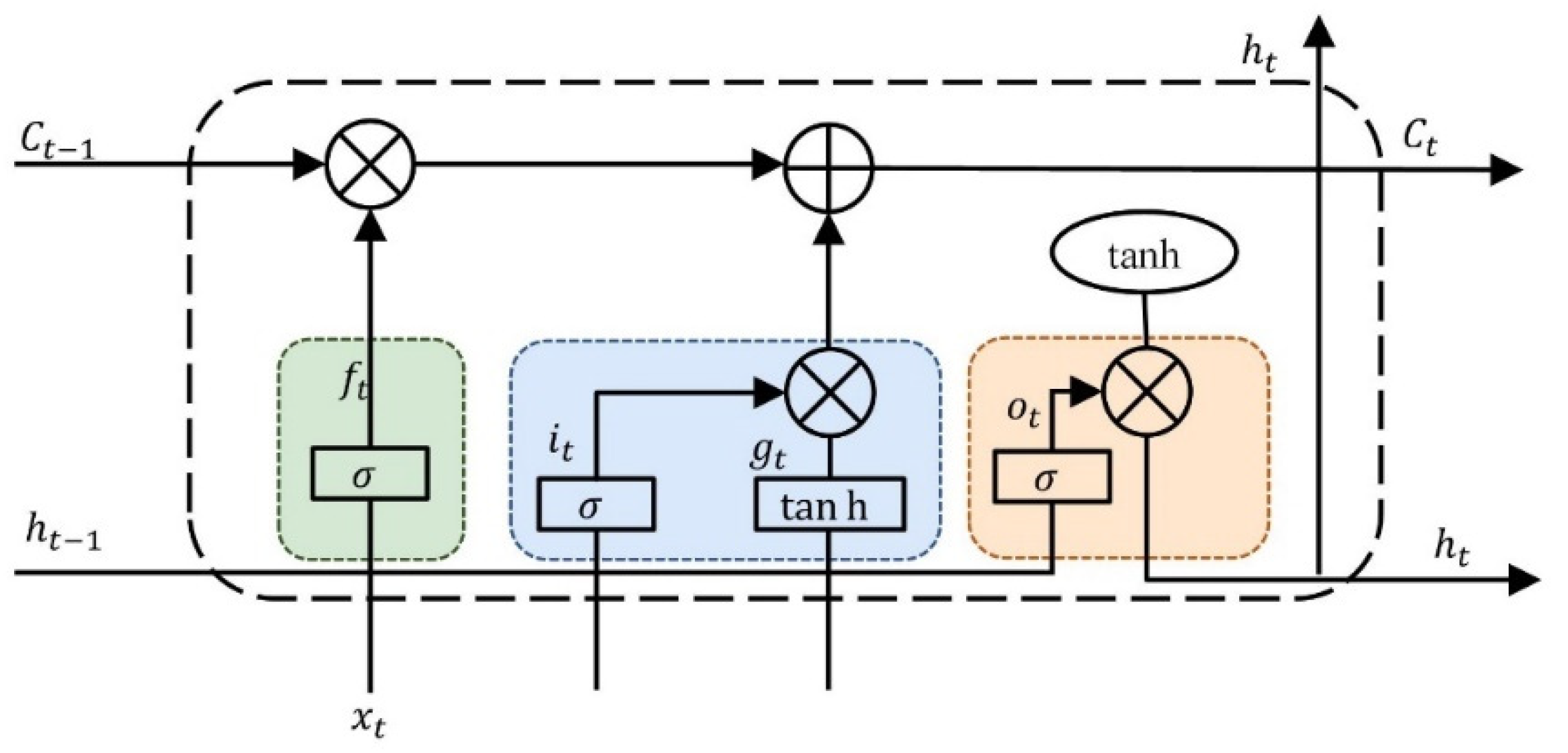
Long short-term memory (LSTM) utilizes three essential gates—input, forget, and output—to control the information flow within its cell state and hidden state. The forget gate manages the removal of past information from the cell state. The input gate regulates the incorporation of new information. The output gate calculates the hidden state for the current time step, based on the filtered, tanh-activated cell state. This mechanism enables LSTM to effectively preserve long-term memory and model long-range dependencies in time series. The LSTM equations are presented in Equations (8)–(13):
f t = σ ( f ˜ t ) = σ ( W x f x t + W h f h t 1 + b f )
i t = σ ( i ˜ t ) = σ ( W x i x t + W h i h t 1 + b i )
g t = tan h ( g ˜ t ) = tan h ( W x g x t + W h g h t 1 + b g )
C t = C t 1 f t + g t i t
o t = σ ( o ˜ t ) = σ ( W x o x t + W h o h t 1 + b o )
h t = o t · tan h ( C t )
In these equations, x t is the input at time t, while h t 1 and C t 1 are the previous hidden and cell states. The sigmoid gates f t (forget), i t (input), and o t (output) control information flow, yielding values between 0 and 1. The tanh function generates the candidate vector g t (values between −1 and 1) representing new information. These components update the cell state to C t and compute the current hidden state h t . All W terms are weight matrices, and b terms are bias vectors. The LSTM structure diagram is presented in Figure 2.
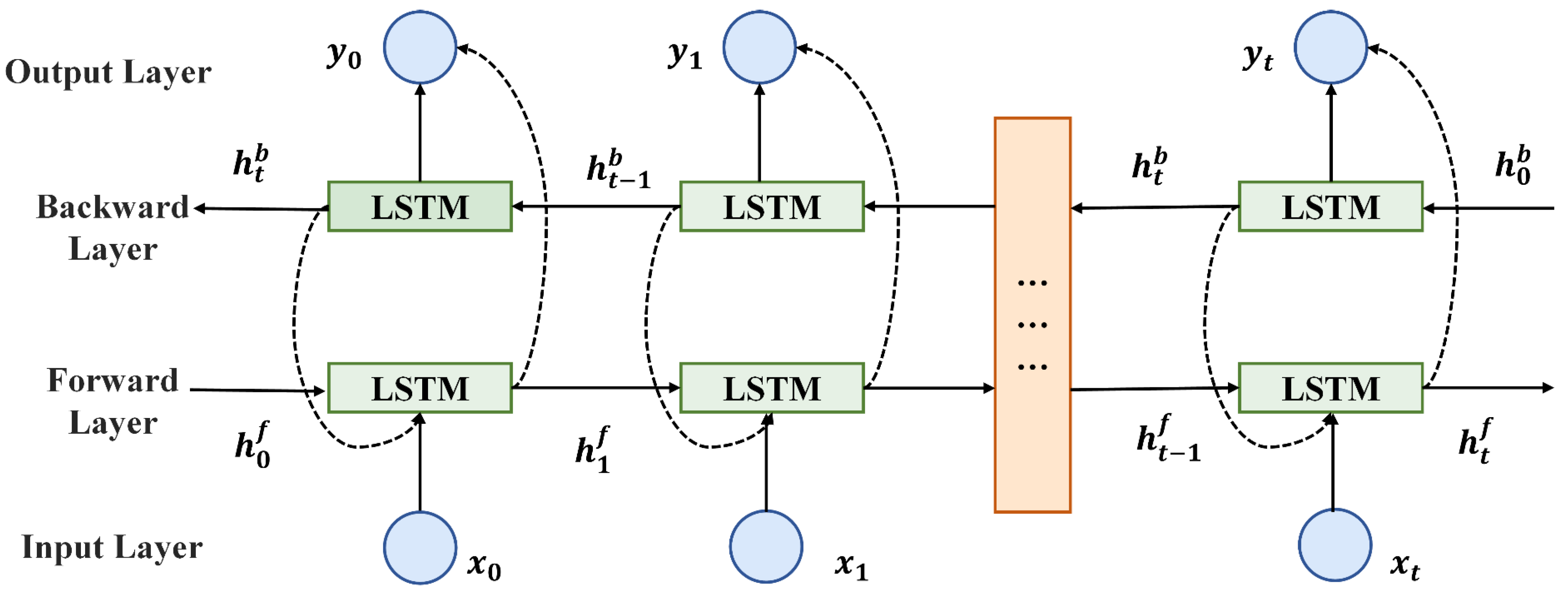
LSTM networks process sequence data primarily relying on past information and the current input for predictions at each time step. This unidirectional nature prevents LSTM from utilizing future context when making predictions, which can limit its overall understanding of the sequence. To overcome this limitation, bidirectional LSTM (Bi-LSTM) was introduced. Bi-LSTM employs a bidirectional architecture, allowing the network to process the entire time series data in both the forward and backward directions. This approach enables Bi-LSTM to capture sequence dependencies more effectively by integrating information from both past and future contexts. The basic structure of Bi-LSTM is depicted in Figure 3.
Bi-LSTM employs two separate LSTM layers sharing the input. The forward layer computes h t f sequentially, while the backward layer computes h t b reversely. Combining these states yields the output h t , integrating past and future information for enhanced data representation compared to standard LSTM. The core computations are as follows:
h t f = L S T M ( x t , h t 1 f )
h t b = L S T M ( x t , h t 1 b )
y t = W 0 h t + b 0
Here, x t is the input at time t, h t f and h t b are the forward and backward hidden states, [ h t f ; h t b ] denotes their concatenation, W 0 and b 0 are the output layer’s weight matrix and bias, and y t = W 0 [ h t f ;   h t b ] + b 0 yields the final prediction.
(2) 
GRU
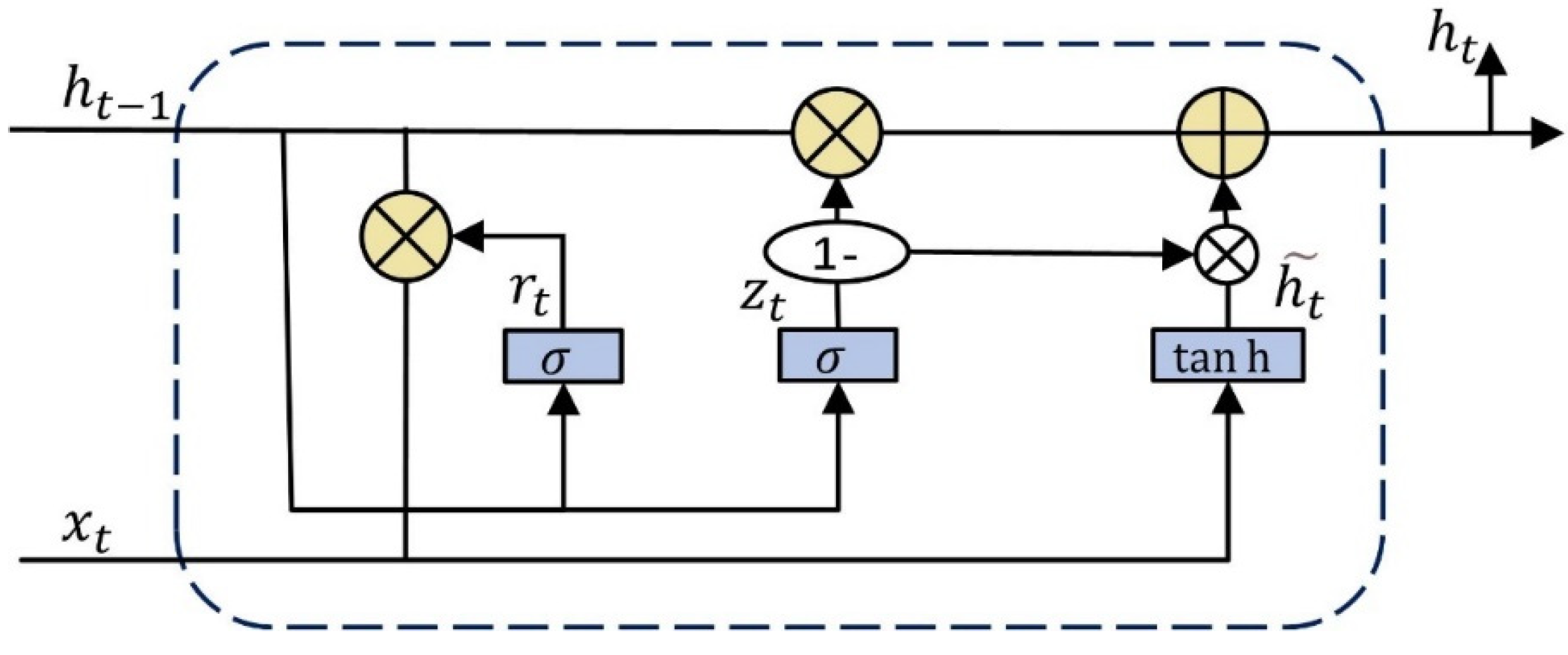
The GRU, introduced by Chung et al. (2014), is an advanced recurrent neural network used for time series forecasting. Unlike LSTM networks, GRU simplifies the architecture with two gating mechanisms: the update gate and the reset gate. This reduces training parameters, lowers computational complexity, and improves training efficiency. Additionally, GRU effectively addresses the vanishing gradient problem in traditional RNNs.
In GRU, the reset gate r t and the update gate z t are computed using the following equations:
r t = σ ( W r · [ h t 1 , x t ] )
z t = σ ( W z · [ h t 1 , x t ] )
The candidate hidden state h t ˜ is calculated as follows:
h t ˜ = tanh ( W h ˜ · [ r t h t 1 , x t ] )
The final hidden state h t is updated using the formula:
h t = z t h t ˜ + ( 1 z t ) h t 1
Here, x t denotes the present input, and h t 1 signifies the hidden state from the preceding time step. Through these computations, GRU adeptly captures temporal dependencies in sequential data, rendering it appropriate for various time series analytic jobs. The structure of the GRU is illustrated in Figure 4.
(3) 
FNN
The FNN (Fang et al., 2023) merges neural network and dynamic systems theory to process time-series data. It uses feedback connections to feed outputs back as inputs or hidden states, providing memory and adaptability for sequential modeling (Nanthakumaran & Tilakaratne, 2018).
FNN consists of an input layer, one or more hidden layers, and an output layer. Neurons in each layer are interconnected through weighted links. The input layer receives raw data, the hidden layer processes it, and the output layer produces the final result.
The input to the hidden layer is expressed as:
h ( t ) = f ( W i h x ( t ) + W f h y ( t 1 ) + b h )
The output of the hidden layer is given by:
y ( t ) = g ( W h o h ( t ) + b o )
where x ( t ) represents the input vector, y ( t ) denotes the output vector, h ( t ) signifies the hidden layer output, while f and g are activation functions. W i h and W f h denote the weight matrices for the input to the hidden layer and feedback connections, respectively, while W h o represents the weight matrix from the hidden layer to the output layer. b h and b o represent the bias vectors.
(4) 
ZOA
The zebra optimization algorithm is a new swarm intelligence optimization technique that solves complex problems by simulating zebra social behavior and migration patterns (Trojovska et al., 2022). Proposed in 2020, it is inspired by the cooperation and coordination zebras exhibit when facing predators, offering valuable insights for optimization algorithm design. The ZOA framework includes population initialization, fitness evaluation, position updating, and iteration.
First, Step One involves initializing the population by randomly generating a set of zebra positions represented as Z = { z 1 , z 2 , , z n } , where n is the population size. Next, Step Two entails evaluating the fitness of each zebra’s position through an objective function f ( z ) , calculating the fitness value as f i t n e s s ( z i ) = f ( z i ) . Building upon this, Step Three updates the position of each zebra based on their interactions and fitness, using the position update formula:
z i n e w = z i o l d + α · ( z b e s t z i ) + β · ( z r a n d o m z i )
Here, z b e s t represents the current best solution, z r a n d o m signifies the location of a randomly chosen zebra, and α and β are control parameters. This process iterates continuously until a predefined termination criterion is satisfied, such as achieving the maximum iteration count or when the change in fitness drops below a set threshold.
Through this methodology, ZOA effectively explores the solution space to identify global optima. Future research can delve into optimizing algorithm parameters and expanding its applicability across various domains to enhance efficiency and accuracy.

3.3. Proposed Model Framework

This section outlines the structure of the proposed model, which includes three main components: (1) data decomposition and reconstruction, (2) a combination weight forecasting model, and (3) model integration and evaluation metrics. The overall architecture is illustrated in Figure 1.
  • Module 1: Data Decomposition and Reconstruction
In this study, historical exchange rate data for selected currency pairs were initially collected. Considering the inherent nonlinearity and nonstationarity of exchange rate series, the OCEEMDAN method was employed for multi-scale decomposition of the original time series. By adaptively adding Gaussian white noise during decomposition, OCEEMDAN effectively mitigates mode mixing and produces IMFs at various scales, along with a residual trend component, thereby facilitating clearer feature extraction for subsequent analyses.
Nevertheless, not all IMFs generated from the decomposition process are beneficial for forecasting, as some predominantly represent noise, potentially impairing prediction accuracy. To address this issue, the study introduces an IMF selection and reconstruction strategy based on sample entropy. Specifically, the sample entropy values of individual IMFs are calculated and utilized to set a threshold. IMFs exhibiting higher entropy values—indicating richer informational content—are retained, whereas those dominated by noise with lower entropy are discarded. Finally, the selected IMFs are recombined to reconstruct a denoised, informative signal, enhancing the reliability and predictive performance of the forecasting model.
  • Module 2: Combination Weight Forecasting Model
In exchange rate prediction, individual forecasting models frequently exhibit limitations in capturing complex data patterns due to their inherent structural constraints, especially when processing nonlinear dependencies or noisy observations. To overcome these challenges, this research develops an ensemble weighting framework that dynamically optimizes sub-model contributions through adaptive weight adjustment, thereby improving both robustness and predictive accuracy. Departing from conventional uniform weighting approaches, this framework implements an intelligent optimization scheme to accommodate data variability, effectively combining diverse model strengths to mitigate prediction errors. The key innovation involves strategic weight distribution to amplify complementary effects among constituent models, yielding enhanced performance in volatile market conditions.
Firstly, this study selects the Bi-LSTM, GRU, and FNN models as the basic models, which stems from their complementary advantages in modeling the multi-scale dynamic characteristics of exchange rates: FNN, with its global nonlinear mapping ability, is good at capturing low-frequency trend components, and its feedforward structure avoids the gradient attenuation problem of recurrent networks in long-term dependent modeling. The bidirectional gating mechanism of Bi-LSTM can effectively extract the nonlinear causal relationship in the high-frequency fluctuation components by jointly encoding historical and potential future information. The simplified gating design of GRU ensures efficiency while enhancing noise robustness, making it perform exceptionally well in the modeling of mid-frequency periodic components.
The combined prediction result is defined as:
y τ ˜ = j = 1 m λ j y j τ
where m indicates the number of base models, λ j signifies the weight coefficient constrained by λ j = 1 and λ j [ 0 , 1 ] , while Λ = ( λ 1 , λ 2 , , λ m ) ^ T constitutes the weight vector. This representation advances beyond simple averaging by quantifying each model’s relative significance.
The optimal weight determination involves minimizing an objective function Ψ :
min Ψ = Λ T B Λ
subject to Γ ^ T   Λ = 1 and Λ 0 , where the composite prediction residual ε τ is defined as:
ε τ = y τ y τ ˜ = j = 1 m λ j ( y τ y j τ ) = j = 1 m λ j ε j τ
Here, ε j τ = y τ y j τ denotes individual model prediction errors, B represents the residual covariance matrix, and Γ = [ 1 , 1 , , 1 ] ^ T is an identity vector. This optimization paradigm establishes quantitative associations between weighting parameters and prediction fidelity through error decomposition analysis.
For improved dynamic adaptation, the ZOA is employed for weight calibration. The enhanced optimization model becomes:
min   Ψ = Λ T B   Λ
with constraints Γ ^ T   Λ = 1 and Λ 0 .
By comparing optimization methods such as ZOA, PSO, GA, and grid search, the experiment found that the two-stage behavior of ZOA simulating zebra foraging and defense strategies can dynamically adapt to market conditions, and it is mostly superior to other algorithms in terms of convergence speed, computational efficiency and stability, and is particularly suitable for this exchange rate prediction task. Therefore, ZOA is used to optimize the integration weights.
The ZOA mimics the collective behavior of zebras to dynamically adjust model weights, balancing contributions from different models. This iterative process enables the ZOA to find the optimal weight combination within the search space, minimizing prediction error. By optimizing the weight combination of Bi-LSTM, GRU, and FNN, the model improves predictive performance, accuracy, and generalization across many datasets, illustrating the efficacy and applicability of this method.
When integrating the Bi-LSTM, GRU, and FNN prediction models using the ZOA, as the contributions of each model in prediction vary, the ZOA is employed to determine their optimal weight combination. It can be analogized as in a weight allocation space, where specific coordinate points denote the weights of subsequences, and the quantity of subsequences aligns with the number of pertinent coordinate points.
The fitness function for determining the optimal weight of the system is as follows:
m i n f ( y ) = M S E = i = 1 n ( y i ^ y i ) 2 n ,   i = 1 , 2 , ,   n
where y i is the initial value, y i ^ is the subsequence prediction value generated by the three models, and i is the subsequence serial number. This function can evaluate the prediction errors under different weight combinations. Based on this, ZOA searches and optimizes in the weight space to find the weight configuration that minimizes the mean square error.
  • Module 3: Model Integration and Evaluation Metrics
After completion of ZOA optimization, the derived optimal weights are integrated with the forecast outcomes of each model to provide the final carbon price prediction result:
F o r e c a s t i n g   r e s u l t = n = 1 3 ω n × r e s u l t n = ω 1 r e s u l t 1 + ω 2 r e s u l t 2 + ω 3 r e s u l t 3
where ω i represents ZOA-optimized weights, and result i corresponds to outputs from Bi-LSTM, GRU, and FNN. This adaptive weighting strategy synergizes Bi-LSTM’s long-term memory, GRU’s gated feature extraction, and FNN’s nonlinear approximation capabilities.
In the evaluation phase, the trained model is utilized on the test set to produce predictions. Four principal measures are employed to evaluate the model’s predictive performance: mean absolute percentage error (MAPE), mean absolute error (MAE), coefficient of determination (R2), and mean square error (MSE). These metrics offer a thorough assessment of the model’s accuracy and error attributes from multiple viewpoints.
M A P E = 1 n i = 1 n | y i y i ^ y i | 100 %
M A E = 1 n i = 1 n | y i y i ^ |
R 2 = 1 i = 1 n ( y i y i ^ ) 2 i = 1 n ( y i y i ¯ ) 2
M S E = 1 n i = 1 n ( y i y i ^ ) 2
In these equations, n the total quantity of data points inside the test set. y i represents the actual value for the, while y i ^ is the anticipated value. y i ¯ represents the average of the actual values in the test set. These variables are utilized to calculate the essential metrics that evaluate the model’s performance, including error magnitude and explained variance.
Furthermore, the improvement of the model is quantified by calculating the percentage change in performance for each evaluation metric. The percentage improvement is determined for the MAPE, mean MAE, MSE, and R2. The formula used to calculate the percentage improvement for each of these metrics is given by:
P m e t r i c ( % ) = ( E b a s e l i n e E i m p r o v e d ) E b a s e l i n e × 100 %
where E b a s e l i n e refers to the error metric (such as MAPE, MAE, MSE, or R 2 of the baseline model, and E i m p r o v e d refers to the error metric of the improved model. This method allows for a clear visualization of the percentage improvement in each evaluation metric, providing a transparent and quantitative basis for assessing the optimization of model performance.

4. Empirical Analysis

This section begins by introducing the data source. The exchange rate series is then analyzed, decomposed using the OCEEMDAN method, and reconstructed to extract meaningful features. The proposed forecasting model is applied to the reconstructed data, and its performance is evaluated through comparisons with traditional models, alternative decomposition methods, and fixed-weight ensembles. Finally, SHAP analysis is conducted to identify key technical indicators influencing exchange rate fluctuations, enhancing the interpretability and practical relevance of the model.

4.1. Experimental Dataset

4.1.1. Data Source

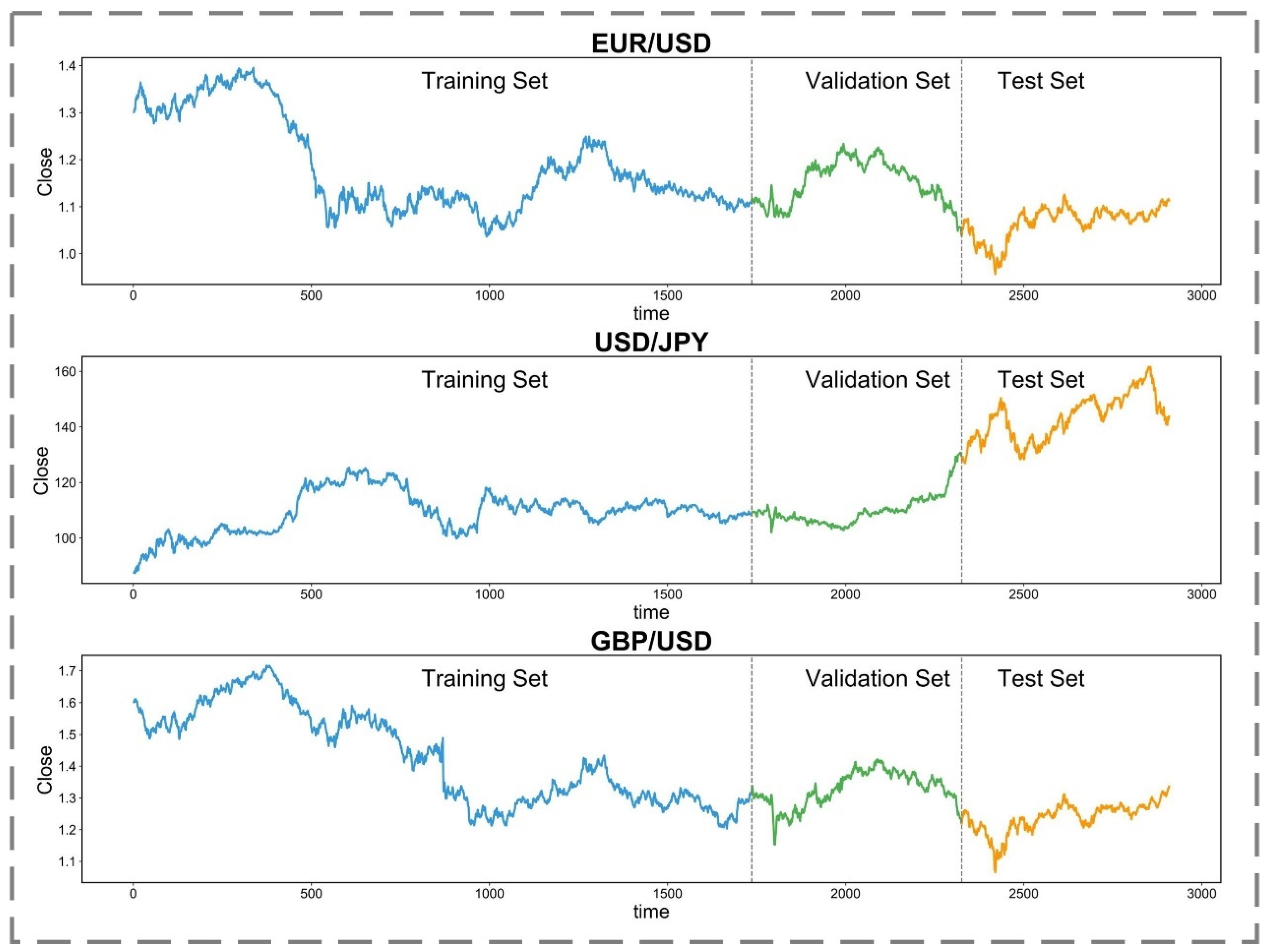
In recent years, the importance of exchange rate prediction has grown, given its critical impact on financial markets and economic policymaking. Accurate forecasting assists investors in making well-informed decisions, helps authorities shape effective monetary strategies, and strengthens risk control mechanisms. This study conducts a case analysis using daily closing prices of three representative currency pairs—EUR/USD, GBP/USD, and USD/JPY—sourced from the Wind database (https://www.wind.com.cn/), accessed on 1 October 2024. The closing prices of these currency pairs function as the prediction objectives. The EUR/USD currency pair data range from 1 January 2013 to 25 September 2024, comprising 2909 entries. The data for the GBP/USD and USD/JPY currency pairs encompass the identical timeframe. No exogenous macroeconomic indicators were incorporated, as the focus was on modeling intrinsic patterns of historical exchange rates. The dataset is partitioned into training, validation, and test sets in a 6:2:2 ratio, as illustrated in Figure 5. Table 1 delineates the sample sizes for the complete dataset, training set, validation set, and test set pertaining to the three currency pairs. Relevant statistical indicators are presented in Table 2.
As shown in Table 2, the standard deviations of the exchange rates are substantial, indicating considerable volatility across the currency pairs. For instance, USD/JPY displays the highest standard deviation of 15.4047, reflecting its greater variability relative to EUR/USD and GBP/USD. The substantial differences between the maximum and minimum values further emphasize this variability, with GBP/USD having a mean of 1.3703, suggesting it is generally stronger than EUR/USD’s average of 1.1560. The non-normal distribution traits of these exchange rates are evident in their kurtosis and skewness values, which demonstrate a rightward skew for all pairs. Overall, these statistics underscore the distinct characteristics and volatility of each currency pair.
Table 3 presents the ADF test results, showing that for all currency pairs, the test statistics exceed the 10% critical threshold, indicating that the null hypothesis of a unit root cannot be rejected. Additionally, all p-values are greater than 0.05, further confirming the presence of unit roots. These findings suggest that the exchange rate series are nonstationary at the 1%, 5%, and 10% significance levels.
Table 4 reports the BDS test results, which assess the nonlinear properties of the EUR/USD, GBP/USD, and USD/JPY exchange rates. As the embedding dimension increases from 2 to 5, the BDS statistics consistently rise. Moreover, with all p-values equal to zero within the 95% confidence interval, strong evidence of nonlinear dependence is observed across all dimensions. This indicates that the dynamics of these currency pairs are influenced by complex, non-random factors, challenging the assumption of market efficiency.

4.1.2. Normalized Processing

To ensure the comparability of input indicators with different dimensions, this study uses the minimum–maximum normalization method to perform linear transformation on the raw data. This process maps each feature to a unified numerical range, eliminating the interference of scale differences on model training while retaining the distribution characteristics of the raw data. The normalization equation is as follows.
x t = x t minX maxX minX
where, x t is a specific value in the original sequence, xt′ is the normalized exchange rate value; minX represents the minimum value in the sequence, and maxX represents the maximum value.

4.2. Decomposition and Reconstruction of Exchange Rate Series

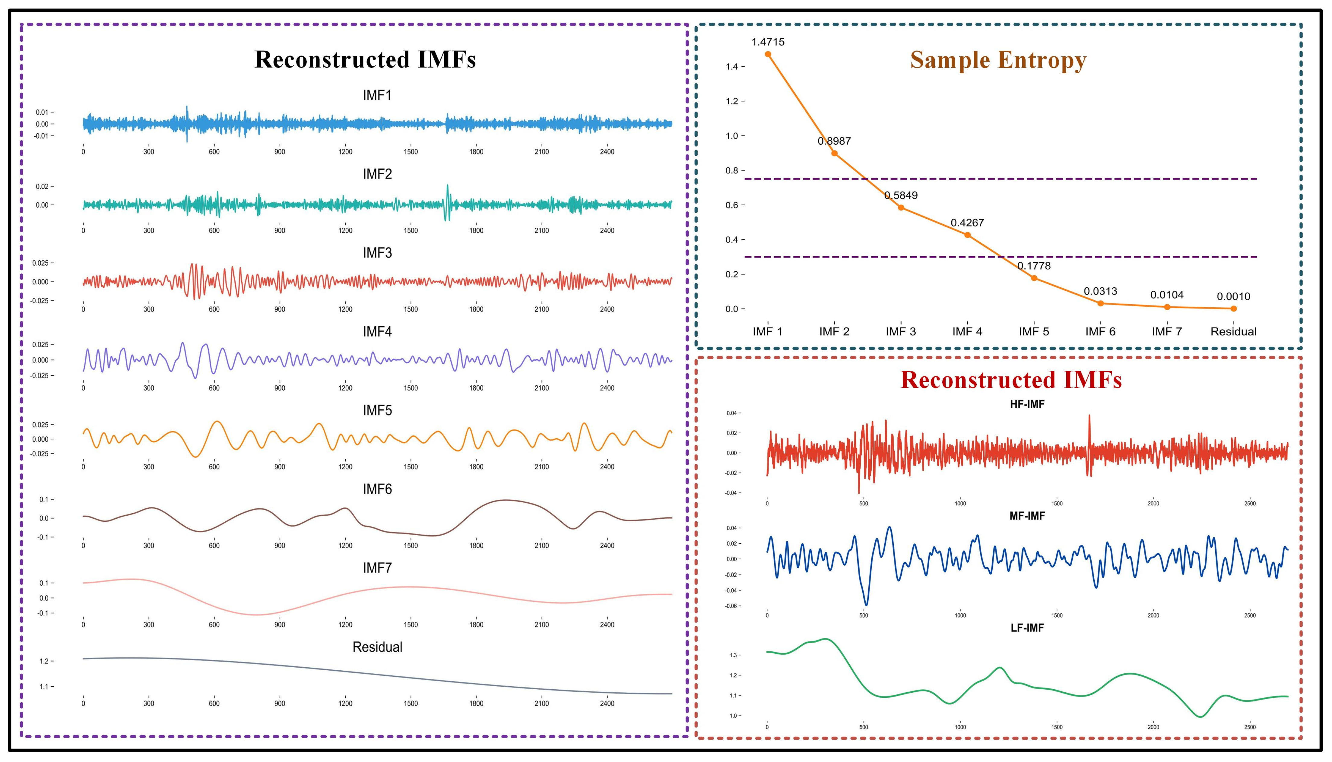
Based on the statistical analysis and tests conducted earlier, the exchange rate series exhibit both nonstationarity and nonlinearity. This section introduces an adaptive parameter-based OCEEMDAN designed for the decomposition of exchange rate time series data. As shown in Figure 6, the EUR/USD series is divided into eight subsequences, with each decomposition mode labeled as IMFi (i = 1, 2, …, 7) accompanied by a residual. Likewise, the initial USD/JPY and GBP/USD series are each partitioned into nine subsequences, and the decomposition structures are illustrated in Figure 7 and Figure 8, respectively.
In addition, to verify robustness, we conducted 10 OCEEMDAN trials on EUR/USD, GBP/USD, and USD/JPY. All series consistently produced 7 to 9 IMFs, confirming the stability of the stop standard in the financial time series.
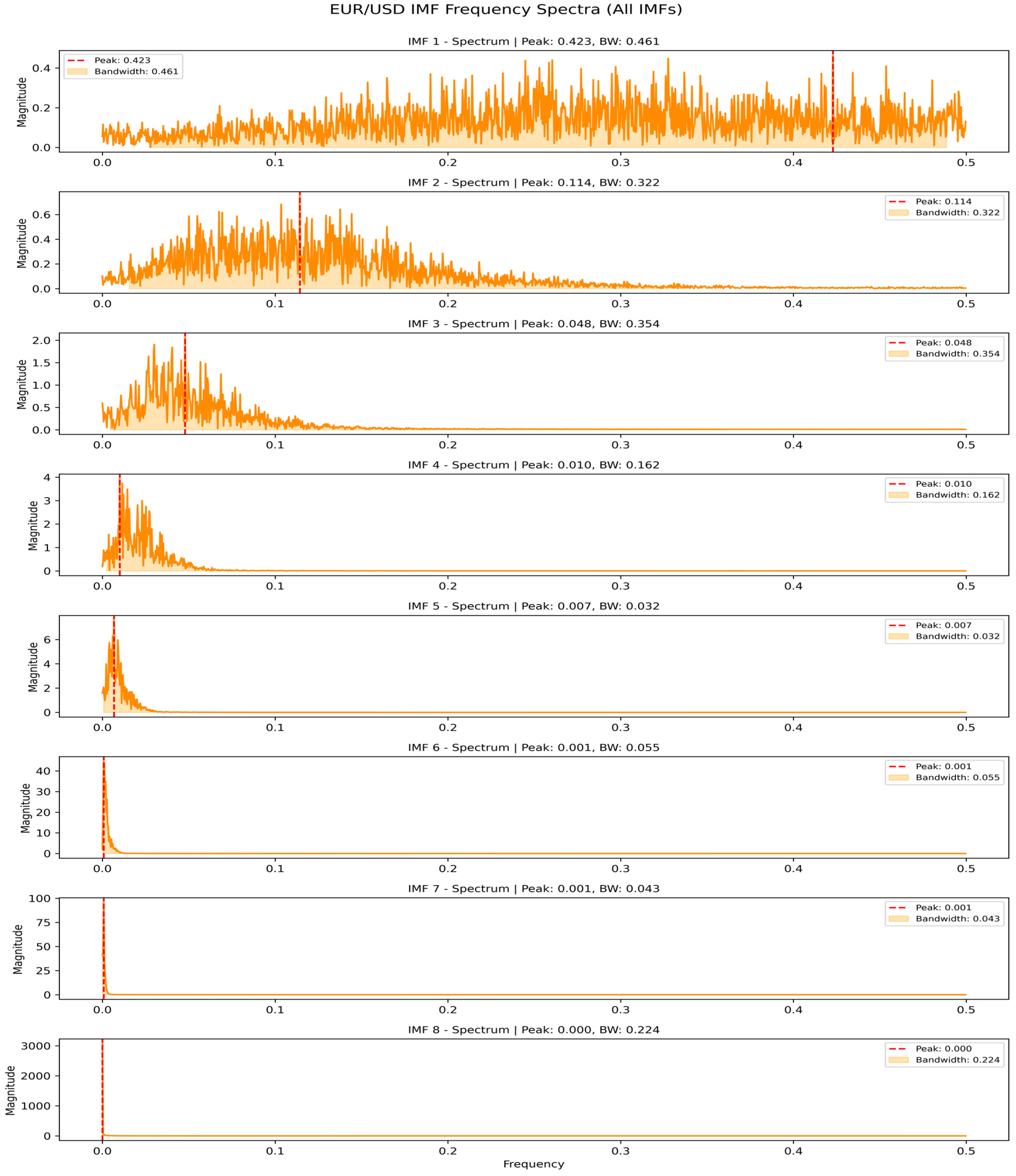
To objectively validate component significance, Figure 9 illustrates the spectral distribution of IMFs for EUR/USD. IMF1–IMF3 exhibit broadband characteristics with distinct peaks, capturing high-frequency market microstructure noise. IMF4–IMF7 demonstrate progressively narrowing bandwidths, isolating economically meaningful cyclical components. IMF8 shows near-zero-frequency dominance, confirming its role as the trend residual. Critically, the entire decomposition process achieves stepwise separation: seven effective modes progressively extract noise, capture cycles, and isolate trends, each component bearing interpretable financial time-series features.
Sample entropy is employed to measure the complexity of various sequences. In this study, the sample entropy of decomposed subsequences is calculated to identify and merge those exhibiting similar complexity, thereby improving reconstruction accuracy and enhancing the understanding of the sequence’s nonlinear characteristics. Taking EUR/USD as an example:
(1)
IMF1 and IMF2 are combined to form the high-frequency component (HF-IMF), which captures random fluctuations in exchange rates and currency pair prices driven by complex trading activities, short-term macroeconomic data releases, and unexpected international financial events (Engle, 2000). Although these high-frequency components contribute to short-term volatility, they typically do not influence long-term trends.
(2)
IMF3 and IMF4 are combined to form the mid-frequency component (MF-IMF), reflecting periodic fluctuations in exchange rates and currency pair prices caused by macroeconomic cycles, monetary policy changes, or international trade dynamics (Borio & Lowe, 2002; Taylor, 1993).
(3)
IMF5, IMF6, IMF7, and the residual are combined to form the low-frequency component (LF-IMF), which is more stable and effectively represents long-term trends in exchange rates and currency pair prices, influenced by global economic structural changes and long-term demographic shifts (Lucas, 2004; Reinhart & Rogoff, 2009).

4.3. Results of the Proposed Model

This study uses the OCEEMDAN methodology to decompose the exchange rate series into several intrinsic mode functions and residual components. Utilizing the attributes of these components, we reconstruct the IMFs, facilitating a more precise depiction of the underlying patterns in the data. We subsequently employ three sophisticated predictive models—Bi-LSTM, GRU, and FNN—to predict the rebuilt sequences. To improve forecast accuracy and stability, we present a new ensemble prediction model, optimized by the ZOA, which identifies the ideal weights for integrating the Bi-LSTM, GRU, and FNN models. This ensemble method facilitates a more dependable and accurate prediction. The hyperparameter configurations of different neural network models are shown in the table in Appendix A.
Figure 10 illustrates the forecasting performance of the proposed model by contrasting predicted values with actual exchange rate data. In the figure, red lines denote the model’s outputs, while blue lines represent observed values. The results show that the model successfully captures the underlying trends in exchange rate movements, performing well in both long-term forecasting and short-term fluctuation tracking. This highlights its effectiveness in modeling the dynamic exchange rate behavior across time horizons. Additionally, the bar chart confirms the model’s superior accuracy and consistency across all datasets.
Table 5 summarizes the performance metrics of the model across the EUR/USD, GBP/USD, and USD/JPY datasets. The results clearly show the exceptional efficacy of the suggested model: regarding the EUR/USD exchange rate, the MAPE, MAE, and MSE are 3.3581%, 2.6501, and 2.1076, respectively, with an R 2 value of 0.9551; for GBP/USD, the MAPE, MAE, and MSE are 3.1683%, 2.5432, and 1.9874, with an R 2 of 0.9231; and for USD/JPY, the MAPE, MAE, and MSE are 2.0945%, 1.8745, and 1.6543, with an R 2 of 0.9180. The results underline the model’s capacity to accurately capture the complex variations of various currency pairs, markedly decreasing prediction errors and exhibiting a high degree of robustness and generalizability across diverse datasets.
In addition, to ensure the statistical reliability of the model performance, we conducted 10 independent experiments for each currency pair, initializing them with different random seeds. The results show that the model has high stability. These statistical results are presented in Appendix B and are consistent with the single-point results in Table 5, further verifying the reliability of the model.
In summary, the ZOA-based weight optimization model exhibits outstanding performance regarding accuracy, stability, and application. It accurately captures long-term patterns and effectively anticipates short-term variations, providing essential decision-making assistance for financial market participants. The model’s strong performance across diverse currency pairs highlights its potential for extensive use in the global financial sector.

5. Further Analysis and Discussion

This section provides further analysis and discussion of the proposed model. It aims to evaluate the model’s overall performance by comparing it with other benchmark models.

5.1. Ablation Study of Key Components

To assess the effectiveness of the proposed model and examine the influence of the OCEEMDAN algorithm on exchange rate forecasting, four sets of ablation experiments are conducted: (1) comparison with traditional single models, (2) comparison with various decomposition methods, (3) comparison with fixed combination weight models, and (4) comparison experiments after removing the sample entropy threshold. Table 6 outlines the assessment metrics for the efficacy of each model in predicting exchange rate series. Table 7 demonstrates the improvement level of each comparative model across different error evaluation metrics. The experimental results indicate the superior performance of the proposed model and provide empirical confirmation for the practical applicability of the OCEEMDAN algorithm in exchange rate forecasting.
Furthermore, Table 8 presents the statistical significance test results of the proposed model compared with three single models. Through two statistical tests, the Diebold–Mariano and Wilcoxon tests, we confirmed that the performance improvement of the proposed model is statistically significant in most cases compared to a single model. At the same time, we also observed that under specific conditions, the advantages of the model may not be statistically significant, which reflects the complexity of the financial market and the dependence of the model’s performance on specific conditions.

5.1.1. Ablation Study on Baseline Model Selection

This section compares the proposed model against three individual models (Bi-LSTM, GRU, and FNN) that predict exchange rate data directly without using decomposition techniques. For the EUR/USD exchange rate, the single models yielded MAPE values of 7.69% (Bi-LSTM), 7.84% (GRU), and 8.47% (FNN). In contrast, the proposed model achieved a significantly lower MAPE of 3.36%. This represents improvements of 4.33%, 4.48%, and 5.12% over Bi-LSTM, GRU, and FNN, respectively. Similar performance gains were observed for the GBP/USD and USD/JPY pairs. The proposed model consistently outperformed the single models across all evaluation metrics (MAPE, MAE, MSE, and R2). For GBP/USD, its MAPE was 3.17%, substantially lower than those of Bi-LSTM (5.91%), GRU (7.13%), and FNN (9.29%). Likewise, for USD/JPY, the proposed model reduced the MAPE to 2.09%, well below the values for Bi-LSTM (4.11%), GRU (5.79%), and FNN (8.56%). The findings confirm the model’s strength in handling complex nonlinear data via decomposition, outperforming single models. This demonstrates its robustness, wide applicability, and consistent accuracy across various exchange rates.

5.1.2. Ablation Study on Decomposition Methods

To further validate the superiority of the proposed IOCEEMDAN-ACWM model, its performance was compared against models based on various single decomposition algorithms, including SSA-ACWM, VMD-ACWM, EEMD-ACWM, and CEEMDAN-ACWM. Using the GBP/USD exchange rate as an example, the proposed model reduced the mean absolute percentage error (MAPE) by 1.99%, 1.39%, 3.64%, and 0.81% compared to SSA-ACWM (5.16%), VMD-ACWM (4.56%), EEMD-ACWM (6.81%), and CEEMDAN-ACWM (3.97%), respectively. This demonstrates a consistent performance advantage.
For additional evaluation, the proposed model was also benchmarked against the secondary decomposition method, CEEMDAN-CEEMDAN-ACWM. Secondary decomposition aims for finer extraction of frequency components through two decomposition rounds to improve accuracy. Indeed, its MAPE for GBP/USD (3.20%) surpassed some single decomposition strategies. However, despite this theoretical advantage in feature extraction, the overall predictive performance of the secondary decomposition method did not exceed that of the proposed model. The proposed model achieved a slightly lower MAPE (3.17%) and also performed better on MAE and MSE metrics. These results suggest that the practical gains from secondary decomposition’s theoretical feature extraction benefits might be limited by its increased computational complexity and challenges in parameter optimization.
Comparative analysis confirms that the proposed model, leveraging OCEEMDAN for superior feature extraction and pattern recognition, comprehensively outperforms benchmark decomposition models. By circumventing the computational and parameter tuning complexities associated with secondary decomposition, the model effectively balances efficiency and accuracy. These findings underscore its theoretical novelty, predictive robustness, and strong practical applicability, positioning it as an efficient and reliable new approach for exchange rate forecasting.

5.1.3. Ablation Study on Sample Entropy Thresholding

To validate the importance of sample entropy thresholding in the framework, we conducted an ablation study by removing this component, resulting in a model named OCEEMDAN-ACWM (No Threshold). This experiment aimed to assess whether the sample entropy-based IMF selection strategy has a substantial contribution to the overall prediction performance. The results presented in Table 6 show that removing the sample entropy thresholding component led to a decline in model performance across all three currency pairs. For example, for EUR/USD, MAPE increased by 16.68% and MSE increased by 92.39%, indicating a deterioration in prediction quality. Similar trends were observed for GBP/USD and USD/JPY, indicating that sample entropy thresholding substantially contributes to prediction performance across all currency pairs. The reason for this lies in the ability of sample entropy thresholding to select information-rich IMFs based on their complexity and combine IMFs with similar complexity into high-frequency, mid-frequency, and low-frequency components, thereby more accurately capturing the intrinsic characteristics of exchange rate data.

5.1.4. Ablation Study on Dynamic Weight Optimization

To further validate the effectiveness of the dynamic weight optimization strategy, this study compares the proposed model against the benchmark fixed combination weight model (OCEEMDAN-FCWM). FCWM is an ensemble prediction method that integrates outputs from multiple sub-models using preset, fixed weights. Comparative analysis reveals that the proposed model, with its dynamic weight adjustment capability, exhibits significant advantages across all tested exchange rates (EUR/USD, GBP/USD, USD/JPY) and evaluation metrics. Taking the USD/JPY prediction as an example, the proposed model reduced the MAPE significantly to 2.09% from OCEEMDAN-FCWM’s 5.88%, a decrease of 3.79 percentage points. Similarly, MAE improved from 3.15 to 1.17 (a reduction of 1.98), and MSE improved from 2.39 to 1.09 (a reduction of 1.30). These quantitative results confirm that the dynamic weight strategy, by adapting to data dynamics, better captures nonlinear and complex patterns compared to FCWM’s fixed-weight design, thus significantly enhancing prediction accuracy.
The comparative study confirms the superiority of the proposed model’s dynamic weight strategy over static weighting. By dynamically adjusting weights, the proposed model more accurately captures evolving data features and patterns, overcoming adaptability limitations and enhancing the efficiency of feature extraction and pattern recognition. These findings highlight the critical role and theoretical/practical significance of dynamic weight adjustment, indicating valuable directions for future research in exchange rate forecasting.

5.2. Risk-Management Applications and Value

The exchange rate forecasting framework developed in this study contributes to risk management in three interconnected ways.
(a)
High-frequency volatility signals extracted from the model’s components, combined with a zero-order allocation (ZOA) weighting scheme, enable real-time adjustment of hedge ratios. When the model anticipates short-term turbulence, derivative exposures can be increased automatically, shielding portfolios from market swings and enhancing risk-adjusted performance.
(b)
Low-frequency trend components extracted via OCEEMDAN, in conjunction with a historical extreme events database, are used to construct a complex systems-based early warning model. This approach facilitates the early detection of nonlinear risk signals, such as exchange rate overshooting or abrupt policy changes, providing valuable data for regulators and firms to initiate stress tests and contingency plans in advance.
(c)
By integrating multiple models and optimizing with information entropy, the predictive framework significantly reduces parameter sensitivity inherent in single models. By quantifying forecast confidence intervals, financial institutions can more accurately assess the uncertainty boundaries of exchange rate predictions, preventing decision-making biases caused by model overfitting and enhancing the scientific rigor and adaptability of risk management practices.

6. Conclusions

This study addresses the key limitations in traditional exchange rate prediction methods by introducing an innovative framework. The framework integrates the OCEEMDAN algorithm and an intelligently optimized combined weight prediction model. By using the GWO to optimize OCEEMDAN’s noise parameters, the accuracy and robustness of signal decomposition are enhanced, revealing deeper insights into exchange rate data. Additionally, the ZOA is employed to dynamically adjust the weights of Bi-LSTM, GRU, and FNN models, forming an adaptive ensemble model that significantly improves prediction performance.
To evaluate the effectiveness of this model, it was compared with ten alternative methods, including the traditional single predictor and the advanced model combined with data decomposition. Through extensive empirical analysis on EUR/USD, GBP/USD, and USD/JPY exchange rates, it has been verified that the proposed framework shows significant improvements in prediction accuracy and robustness compared with existing methods. This study’s principal contributions are as follows:
  • We proposed applying the GWO to the automatic optimization of key parameters of CEEMDAN for financial time series prediction.
  • A framework for exchange rate prediction using the zebra optimization algorithm for dynamic integrated weight optimization was proposed. ZOA’s two-stage behavior of simulating zebra foraging and defense strategies makes it particularly suitable for balancing exploration and development in a weighted space.
  • The developed exchange rate prediction model, verified through historical simulations, has demonstrated its stability and reliability under various market conditions.
Several potential avenues for future research can be explored to enhance the practical applicability of our framework. First, we will optimize the model for real-time trading through quantization and pruning and extend it to multi-output scenarios via multi-task learning. Second, parallel computing and GPU acceleration will be investigated to improve computational efficiency. Third, the framework’s performance on volatile and low-liquidity currency pairs will be evaluated by adjusting the IMF selection criteria. Finally, we plan to extend the framework to high-frequency forecasting and cross-market applications, including stock indices and commodity prices, to develop a unified forecasting framework for diverse financial time series.

Author Contributions

X.T.: conceptualization, data curation, formal analysis, investigation, methodology, software, validation, visualization, writing—original draft. Y.X.: conceptualization, funding acquisition, project administration, resources, supervision, writing—review and editing. All authors have read and agreed to the published version of the manuscript.

Funding

The research reported was supported by the Postgraduate Research & Practice Innovation Program of Jiangsu Province (KYCX25_2594).

Data Availability Statement

Data available upon request from the authors.

Conflicts of Interest

The authors declare that they have no known competing financial interests or personal relationships that could have appeared to influence the work reported in this paper.

Abbreviations

ADFAugmented dickey-fuller
ALSTMAttention-based long short-term memory
APSOAccelerated particle swarm optimization
ARIMAAutoregressive integrated moving average
CEEMDComplete ensemble empirical mode decomposition
CEEMDANComplete ensemble empirical mode decomposition with adaptive noise
CNNConvolutional neural network
DEDifferential evolution
EEMDEnsemble empirical mode decomposition
EMDEmpirical mode decomposition
GANGenerative adversarial network
GARCHGeneralized autoregressive conditional heteroskedasticity
GRUGated recurrent unit neural network
GWOGrey wolf optimizer
IEInformation entropy
IMFIntrinsic mode function
IWOAImproved whale optimization algorithm
LSTMLong short-term memory
MAEMean absolute error
MAPEMean absolute percentage error
OCEEMDANOptimal complete ensemble empirical mode decomposition with adaptive noise
PSOParticle swarm optimization
RMSERoot-mean-square error
RNNRecurrent neural networks
R2Coefficient of determination
SESample entropy
SSASingular spectrum analysis
VARVector autoregression
WTWavelet transform
ZOAZebra optimization algorithm

Appendix A. Neural Network Model Hyperparameter Configurations for Three Exchange Rates

ModelParameterEUR/USDGBP/USDUSD/JPY
Bi-LSTMHidden layers232
Units per layer100128256
Dropout rate0.150.30.25
Learning rate0.0010.00050.0015
Batch size643248
Gradient clipping121.5
L2 regularization0.00010.00030.0002
GRUHidden layers223
Units per layer128100200
Dropout rate0.20.250.3
Learning rate0.00080.00070.0005
Batch size324824
Gradient clipping1.211.8
L2 regularization0.000150.00020.00025
FNNHidden layers343
Neurons per layer[256,128,64][300,150,75,38][400,200,100]
Dropout rate0.30.40.35
Hidden layer activationReLULeakyReLUReLU
Output activationLinearLinearLinear
Learning rate0.0010.00060.0012
Batch size643248
L2 regularization0.00010.000250.00015

Appendix B. Statistical Analysis of the Proposed Model

MAPE (%)MAEMSER2
EUR/USD3.3581 ± 0.1245
(3.2336–3.4826)
2.6501 ± 0.0937
(2.5564–2.7438)
2.1076 ± 0.0745
(2.0331–2.1821)
0.9551 ± 0.0042
(0.9509–0.9593)
GBP/USD3.1683 ± 0.1032
(3.0651–3.2715)
1.5493 ± 0.0508
(1.4985–1.5999)
1.6174 ± 0.0530
(1.5644–1.6704)
0.9231 ± 0.0040
(0.9191–0.9271)
USD/JPY2.0945 ± 0.0723
(2.0222–2.1668)
1.1659 ± 0.0403
(1.1256–1.2062)
1.0945 ± 0.0379
(1.0566–1.1324)
0.9180 ± 0.0035
(0.9145–0.9215)

References

  1. Alexandridis, A. K., Panopoulou, E., & Souropanis, I. (2024). Forecasting exchange rate volatility: An amalgamation approach. Journal of International Financial Markets, Institutions and Money, 97, 102067. [Google Scholar] [CrossRef]
  2. Borio, C. E. V., & Lowe, P. W. (2002). Asset prices, financial and monetary stability: Exploring the nexus. SSRN Journal. [Google Scholar] [CrossRef]
  3. Chung, J., Gulcehre, C., Cho, K., & Bengio, Y. (2014). Empirical evaluation of gated recurrent neural networks on sequence modeling. arXiv. [Google Scholar] [CrossRef]
  4. Ding, H., Zhao, X., Jiang, Z., Abdullah, S. N., & Dewi, D. A. (2024). EUR-USD exchange rate forecasting based on information fusion with large language models and deep learning methods. arXiv. [Google Scholar] [CrossRef]
  5. Du, P., Ye, Y., Wu, H., & Wang, J. (2025). Study on deterministic and interval forecasting of electricity load based on multi-objective whale optimization algorithm and transformer model. Expert Systems with Applications, 268, 126361. [Google Scholar] [CrossRef]
  6. Engle, R. F. (2000). Dynamic conditional correlation—A simple class of multivariate GARCH models. Journal of Business & Economic Statistics, 20(3), 339–350. [Google Scholar] [CrossRef]
  7. Fang, T., Zheng, C., & Wang, D. (2023). Forecasting the crude oil prices with an EMD-ISBM-FNN model. Energy, 263, 125407. [Google Scholar] [CrossRef]
  8. Ghosh, I., & Dragan, P. (2023). Can financial stress be anticipated and explained? Uncovering the hidden pattern using EEMD-LSTM, EEMD-prophet, and XAI methodologies. Complex & Intelligent Systems, 9, 4169–4193. [Google Scholar] [CrossRef]
  9. Gong, M., Zhao, Y., Sun, J., Han, C., Sun, G., & Yan, B. (2022). Load forecasting of district heating system based on Informer. Energy, 253, 124179. [Google Scholar] [CrossRef]
  10. Gui, Z., Li, H., Xu, S., & Chen, Y. (2023). A novel decomposed-ensemble time series forecasting framework: Capturing underlying volatility information. arXiv. [Google Scholar] [CrossRef]
  11. Hochreiter, S., & Schmidhuber, J. (1997). Long short-term memory. Neural Computation, 9, 1735–1780. [Google Scholar] [CrossRef]
  12. Lee, M.-C. (2022). Research on the feasibility of applying GRU and attention mechanism combined with technical indicators in stock trading strategies. Applied Sciences, 12, 1007. [Google Scholar] [CrossRef]
  13. Liu, P., Wang, Z., Liu, D., Wang, J., & Wang, T. (2023). A CNN-STLSTM-AM model for forecasting USD/RMB exchange rate. Journal of Engineering Research, 11, 100079. [Google Scholar] [CrossRef]
  14. Liu, S., Huang, Q., Li, M., & Wei, Y. (2024). A new LASSO-BiLSTM-based ensemble learning approach for exchange rate forecasting. Engineering Applications of Artificial Intelligence, 127, 107305. [Google Scholar] [CrossRef]
  15. Lu, H., Ma, X., Huang, K., & Azimi, M. (2020). Carbon trading volume and price forecasting in China using multiple machine learning models. Journal of Cleaner Production, 249, 119386. [Google Scholar] [CrossRef]
  16. Lucas, R. (2004). The industrial revolution: Past and future. Available online: https://www.aier.org (accessed on 20 May 2025).
  17. Luo, J., & Gong, Y. (2023). Air pollutant prediction based on ARIMA-WOA-LSTM model. Atmospheric Pollution Research, 14, 101761. [Google Scholar] [CrossRef]
  18. Mroua, M., & Lamine, A. (2023). Financial time series prediction under COVID-19 pandemic crisis with long short-term memory (LSTM) network. Humanities and Social Sciences Communications, 10, 530. [Google Scholar] [CrossRef]
  19. Nanthakumaran, P., & Tilakaratne, C. D. (2018). Financial time series forecasting using empirical mode decomposition and FNN: A study on selected foreign exchange rates. International Journal on Advances in ICT for Emerging Regions, 11, 1–12. [Google Scholar] [CrossRef]
  20. Oreshkin, B. N., Carpov, D., Chapados, N., & Bengio, Y. (2020). N-BEATS: Neural basis expansion analysis for interpretable time series forecasting. arXiv. [Google Scholar] [CrossRef]
  21. Pfahler, J. F. (2021). Exchange rate forecasting with advanced machine learning methods. Journal of Risk and Financial Management, 15, 2. [Google Scholar] [CrossRef]
  22. Reinhart, C. M., & Rogoff, K. S. (2009). This time is different: Eight centuries of financial folly. Princeton University Press. [Google Scholar] [CrossRef]
  23. Ren, Y., Huang, Y., Wang, Y., Xia, L., & Wu, D. (2025). Forecasting carbon price in Hubei Province using a mixed neural model based on mutual information and multi-head self-attention. Journal of Cleaner Production, 494, 144960. [Google Scholar] [CrossRef]
  24. Ren, Y., Wang, Y., Xia, L., & Wu, D. (2024). An innovative information accumulation multivariable grey model and its application in China’s renewable energy generation forecasting. Expert Systems with Applications, 252, 124130. [Google Scholar] [CrossRef]
  25. Rezaei, H., Faaljou, H., & Mansourfar, G. (2021). Stock price prediction using deep learning and frequency decomposition. Expert Systems with Applications, 169, 114332. [Google Scholar] [CrossRef]
  26. Semenov, A. (2024). Overreaction and underreaction to new information and the directional forecast of exchange rates. International Review of Economics & Finance, 96, 103676. [Google Scholar] [CrossRef]
  27. Taylor, J. B. (1993). Discretion versus policy rules in practice. Carnegie-Rochester Conference Series on Public Policy, 39, 195–214. [Google Scholar] [CrossRef]
  28. Torres, M. E., Colominas, M. A., Schlotthauer, G., & Flandrin, P. (2011, May 22–27). A complete ensemble empirical mode decomposition with adaptive noise. 2011 IEEE International Conference on Acoustics, Speech and Signal Processing (ICASSP) (pp. 4144–4147), Prague, Czech Republic. [Google Scholar] [CrossRef]
  29. Trojovska, E., Dehghani, M., & Trojovsky, P. (2022). Zebra optimization algorithm: A new bio-inspired optimization algorithm for solving optimization algorithm. IEEE Access, 10, 49445–49473. [Google Scholar] [CrossRef]
  30. Wang, J., & Zhang, Y. (2025). A hybrid system with optimized decomposition on random deep learning model for crude oil futures forecasting. Expert Systems with Applications, 272, 126706. [Google Scholar] [CrossRef]
  31. Wang, X., Li, C., Yi, C., Xu, X., Wang, J., & Zhang, Y. (2022). EcoForecast: An interpretable data-driven approach for short-term macroeconomic forecasting using N-BEATS neural network. Engineering Applications of Artificial Intelligence, 114, 105072. [Google Scholar] [CrossRef]
  32. Wu, F., Cattani, C., Song, W., & Zio, E. (2020). Fractional ARIMA with an improved cuckoo search optimization for the efficient Short-term power load forecasting. Alexandria Engineering Journal, 59, 3111–3118. [Google Scholar] [CrossRef]
  33. Wu, P., Zou, D., Zhang, G., & Liu, H. (2024). An improved NSGA-II for the dynamic economic emission dispatch with the charging/discharging of plug-in electric vehicles and home-distributed photovoltaic generation. Energy Science & Engineering, 12, 1699–1727. [Google Scholar] [CrossRef]
  34. Yang, Q., & Li, J. (Eds.). (2025). The proceedings of the 11th Frontier Academic Forum of Electrical Engineering (FAFEE2024): Volume I, lecture notes in electrical engineering. Springer Nature. [Google Scholar] [CrossRef]
  35. Yao, D., Chen, S., Dong, S., & Qin, J. (2024). Modeling abrupt changes in mine water inflow trends: A CEEMDAN-based multi-model prediction approach. Journal of Cleaner Production, 439, 140809. [Google Scholar] [CrossRef]
  36. Yeh, J.-R., Shieh, J. S., & Huang, N. E. (2010). Complementary ensemble empirical mode decomposition: A novel noise enhanced data analysis method. Advances in Data Science and Adaptive Analysis, 2, 135–156. [Google Scholar] [CrossRef]
  37. Zhang, X. (2023). An enhanced decomposition integration model for deterministic and probabilistic carbon price prediction based on two-stage feature extraction and intelligent weight optimization. Journal of Cleaner Production, 415, 137791. [Google Scholar] [CrossRef]
  38. Zhang, Y., Zhong, K., Xie, X., Huang, Y., Han, S., Liu, G., & Chen, Z. (2025). VMD-ConvTSMixer: Spatiotemporal channel mixing model for non-stationary time series forecasting. Expert Systems with Applications, 271, 126535. [Google Scholar] [CrossRef]
  39. Zhou, H., Zhang, S., Peng, J., Zhang, S., Li, J., Xiong, H., & Zhang, W. (2021). Informer: Beyond efficient transformer for long sequence time-series forecasting. arXiv. [Google Scholar] [CrossRef]
  40. Zhou, M. (2024). Predict stock price fluctuations using realized volatility, CEEMDAN, LSTM models. SHS Web of Conferences, 196, 02003. [Google Scholar] [CrossRef]
  41. Zhou, T., Ma, Z., Wen, Q., Wang, X., Sun, L., & Jin, R. (2022). FEDformer: Frequency enhanced decomposed transformer for long-term series forecasting. arXiv. [Google Scholar] [CrossRef]
  42. Zhou, Y., & Zhu, X. (2025). Forecasting USD/RMB exchange rate using the ICEEMDAN-CNN-LSTM model. Journal of Forecasting, 44, 200–215. [Google Scholar] [CrossRef]
  43. Zinenko, A. (2023). Forecasting financial time series using singular spectrum analysis. Business Informatics, 17, 87–100. [Google Scholar] [CrossRef]
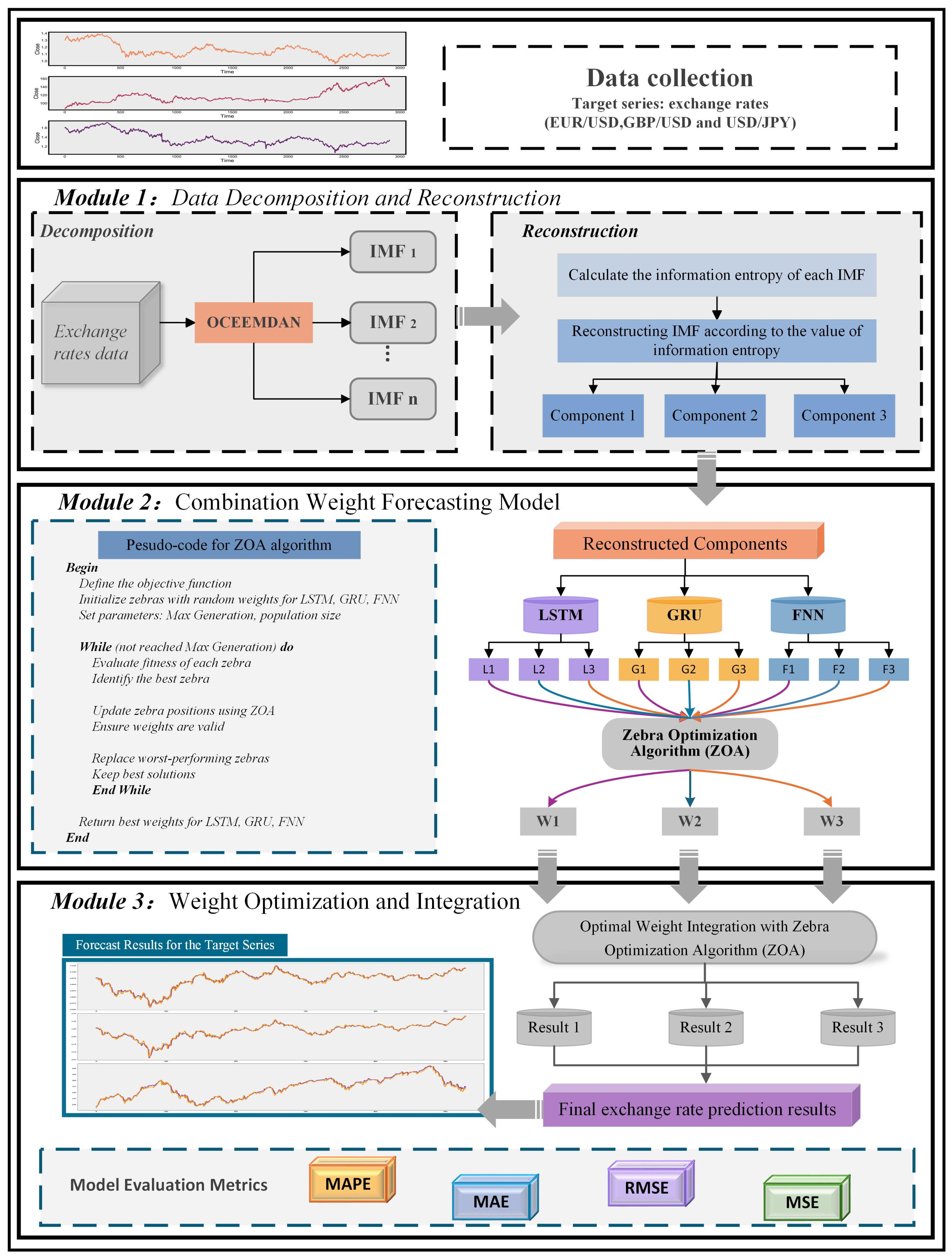
Figure 1. The flowchart of the proposed model.
Ijfs 13 00151 g001
Figure 2. The structure of LSTM.
Ijfs 13 00151 g002
Figure 3. The structure of Bi-LSTM.
Ijfs 13 00151 g003
Figure 4. The structure of GRU.
Ijfs 13 00151 g004
Figure 5. Exchange rate data and dataset splits.
Ijfs 13 00151 g005
Figure 6. Decomposition and reconstruction of the daily EUR/USD exchange rate.
Ijfs 13 00151 g006
Figure 7. Decomposition and reconstruction of the daily GBP/USD exchange rate.
Ijfs 13 00151 g007
Figure 8. Decomposition and reconstruction of the daily USD/JPY exchange rate.
Ijfs 13 00151 g008
Figure 9. IMF spectral distribution of EUR/USD.
Ijfs 13 00151 g009
Figure 10. The prediction results and evaluation of the dataset.
Ijfs 13 00151 g010
Table 1. Data partition for currency pair prediction models.
Currency PairSample SizeTraining SetValidation SetTest Set
EUR/USD29091745582582
USD/JPY29091745582582
GBP/USD29091745582582
Table 2. Descriptive statistics for exchange rate data.
Currency PairMaxMinMeanStandard DeviationSkewnessKurtosis
EUR/USD1.39530.95651.15600.09340.92580.1019
USD/JPY161.640087.4500116.219815.40471.11370.3684
GBP/USD1.71611.48831.37030.14040.7550−0.5028
Table 3. Results of ADF tests for exchange rates.
Currency PairT-StatisticProb.
EUR/USD−1.960.30
USD/JPY−1.300.63
GBP/USD−1.950.31
Table 4. BDS tests.
Table 4. BDS tests.
Currency PairStatisticZ-Statisticp-Value
EUR/USDBDS (2)5.500.00
BDS (3)9.270.00
BDS (4)15.110.00
BDS (5)21.000.00
GBP/USDBDS (2)6.200.00
BDS (3)11.540.00
BDS (4)18.310.00
BDS (5)24.400.00
USD/JPYBDS (2)8.590.00
BDS (3)7.330.00
BDS (4)15.820.00
BDS (5)19.480.00
Table 5. The evaluation results of the proposed model.
Exchange Rate PairsMAPE (%)MAEMSE R 2
Daily EUR/USD exchange rate3.35812.65012.10760.9551
Daily GBP/USD exchange rate3.16831.54931.61740.9231
Daily USD/JPY exchange rate2.09451.16591.09450.9180
Table 6. Comparative analysis of predictive performance across several models.
Exchange Rate PairsModelMAPE (%)MAEMSE R 2
Daily EUR/USD exchange rateBi-LSTM7.68944.15724.48910.8751
GRU7.83926.50275.17430.9401
FNN8.47385.32653.95240.9804
SSA-ACWM5.98724.01434.56380.8946
VMD-ACWM5.08143.47293.10950.7457
EEMD-ACWM4.20343.75823.62910.8947
CEEMDAN-ACWM4.81733.03923.08450.9104
CEEMDAN-CEEMDAN-ACWM3.60193.48212.84670.8142
OCEEMDAN-FCWM5.27513.75942.23050.9238
OCEEMDAN-ACWM(NT)3.91832.60224.05490.8628
Proposed model3.35812.65012.10760.9551
Daily GBP/USD exchange rateBi-LSTM5.91455.61873.98540.8942
GRU7.12545.61474.90760.7193
FNN9.28906.73095.13480.9728
SSA-ACWM5.15712.48233.19580.9074
VMD-ACWM4.56193.82462.43970.8728
EEMD-ACWM6.81243.19433.53890.8067
CEEMDAN-ACWM3.97352.25182.30810.9426
CEEMDAN-CEEMDAN-ACWM3.19792.50831.89450.9698
OCEEMDAN-FCWM5.39263.62142.21730.8047
OCEEMDAN-ACWM(NT)4.18543.86242.98390.8841
Proposed model3.16831.54931.61740.9231
Daily USD/JPY exchange rate Bi-LSTM4.1053 4.40253.12690.9027
GRU5.79317.84124.67830.9115
FNN8.56275.95764.51940.8461
SSA-ACWM4.68533.84713.19340.8428
VMD-ACWM2.38422.62982.41050.9057
EEMD-ACWM3.20634.73493.48120.7257
CEEMDAN-ACWM2.63082.78411.57390.9149
CEEMDAN-CEEMDAN-ACWM3.08592.07351.53820.8561
OCEEMDAN-FCWM5.88123.14962.39480.7939
OCEEMDAN-ACWM(NT)3.11582.09041.58270.8267
Proposed model2.09451.16591.09450.9180
Table 7. The enhancement degree across several mistake assessment measures.
Exchange Rate PairsModel P M A P E (%) P M A E (%) P M S E (%) P R 2
Daily EUR/USD exchange rateBi-LSTM128.06%57.08%112.67%−8.37%
GRU133.60%146.56%145.93%−1.57%
FNN152.72%101.34%87.56%2.66%
SSA-ACWM78.19%51.42%116.50%−6.34%
VMD-ACWM51.12%31.11%47.55%−21.97%
EEMD-ACWM25.13%41.84%72.15%−6.33%
CEEMDAN-ACWM43.41%14.72%46.37%−4.69%
CEEMDAN-CEEMDAN-ACWM7.25%31.42%35.03%−14.74%
OCEEMDAN-ACWM(NT)25.72%30.78%−81.79%−6.60%
OCEEMDAN-FCWM56.94%41.88%5.82%−3.29%
Daily GBP/USD exchange rateBi-LSTM86.91%262.44%146.50%−8.13%
GRU125.07%262.42%203.48%−26.07%
FNN192.82%334.84%217.72%−0.03%
SSA-ACWM62.83%60.24%97.65%−6.77%
VMD-ACWM44.04%147.49%50.87%−10.28%
EEMD-ACWM114.91%106.82%118.94%−17.13%
CEEMDAN-ACWM25.41%45.44%42.77%−3.13%
CEEMDAN-CEEMDAN-ACWM0.94%62.04%17.15%−0.34%
OCEEMDAN-ACWM(NT)38.56%37.59%49.08%1.73%
OCEEMDAN-FCWM70.18%133.63%37.13%−17.28%
Daily USD/JPY exchange rate Bi-LSTM96.02%278.99%185.57%−1.66%
GRU177.57%573.74%327.27%−0.71%
FNN309.77%411.83%313.78%−7.82%
SSA-ACWM123.71%230.78%192.02%−8.18%
VMD-ACWM13.84%125.34%120.61%−1.34%
EEMD-ACWM53.24%305.62%218.96%−21.00%
CEEMDAN-ACWM25.58%138.00%44.02%−0.33%
CEEMDAN-CEEMDAN-ACWM47.43%78.01%40.67%−6.74%
OCEEMDAN-ACWM(NT)64.35%62.98%54.30%15.63%
OCEEMDAN-FCWM180.53%170.72%118.73%−13.54%
Table 8. Statistical significance test results.
ComparisonCurrency PairDM StatisticDM p-ValueWilcoxon StatisticWilcoxon p-Value
Ensemble Model vs. Bi-LSTMEUR/USD3.8420.000126,3420.0002
GBP/USD1.6340.102214,3270.1128
USD/JPY2.7680.005721,8940.0048
Ensemble Model vs. GRUEUR/USD2.3570.018318,5610.0165
GBP/USD4.105<0.000127,178<0.0001
USD/JPY1.2150.224311,2450.2468
Ensemble Model vs. FNNEUR/USD4.721<0.000129,875<0.0001
GBP/USD4.102<0.000127,436<0.0001
USD/JPY3.956<0.000128,145<0.0001
Disclaimer/Publisher’s Note: The statements, opinions and data contained in all publications are solely those of the individual author(s) and contributor(s) and not of MDPI and/or the editor(s). MDPI and/or the editor(s) disclaim responsibility for any injury to people or property resulting from any ideas, methods, instructions or products referred to in the content.